


1. Introduction
Network growth models are fundamental to representing and understanding the evolution of real networks, such as the brain, the web, or online social networks [Reference Newman13]. Traditional growth models such as the celebrated Barabási–Albert model [Reference Barabási and Albert3] often rely on global mechanisms (e.g. they connect to a randomly chosen node) in order to induce properties frequently observed in real networks, such as a heavy-tailed degree distribution or logarithmic node distances. However, many real networks grow out of local mechanisms embodied by processes that unfold on the network. For example, the growth of brain networks is governed by action potentials in neurons [Reference Sporns15], and ties in online social networks are driven by local interactions among users [Reference Kumar, Novak, Tomkins and Yu11,Reference Weng, Ratkiewicz, Perra, Gonçalves, Castillo, Bonchi, Schifanella, Menczer and Flammini17].
Over the past decade, various network models leveraging local mechanisms have been proposed and shown to capture structural properties found in real networks [Reference Cannings and Jordan5,Reference Ikeda10,Reference Li, Gao, Fan, Wu and Di12,Reference Saramäki and Kaski14,Reference Vázquez16]. However, while these models embody local attachment rules, they also rely on some global step, such as choosing a node at random across the entire network. Once a node is chosen, local attachment rules determine the edges to be added locally. Intuitively, this global step ensures that the network can continue to grow in every corner. But is this necessary? Can a purely local growth process give rise to a rich network structure?
This current work tackles this question, providing a positive answer with a surprisingly simple model: a network growth process governed by a random walk and a local attachment rule that connects a new leaf node to the current walker position. In particular, the proposed model can be described algorithmically as follows.
0. Start with an initial network (e.g. a single node with a self-loop) and a random walk placed on one of its nodes.
1. Let the random walk take exactly s steps on the current network.
2. Connect a new node with degree one (i.e. a leaf node) to the current walker node.
3. Go to step 1.
The model is named ‘no restart random walk’ (NRRW) because it builds on previous models in which the random walk would restart (by choosing a node uniformly at random) under certain conditions (e.g. adding a new node) [Reference Cannings and Jordan5,Reference Saramäki and Kaski14]. Note that NRRW is parsimonious and has a single parameter s, called the step parameter. While the initial network is also a parameter, it does not play a prominent role in the structural properties observed asymptotically (as we soon show).
What networks will NRRW generate? Figure 1 depicts networks generated by simulating NRRW for
 ${s}=1$
and
${s}=1$
and
 ${s}=2$
for different numbers of nodes. Clearly, networks generated for
${s}=2$
for different numbers of nodes. Clearly, networks generated for
 $s=1$
and
$s=1$
and
 $s=2$
are very different. As it turns out, the parity of s and its magnitude play a fundamental role in the walker dynamics and the network structure.
$s=2$
are very different. As it turns out, the parity of s and its magnitude play a fundamental role in the walker dynamics and the network structure.
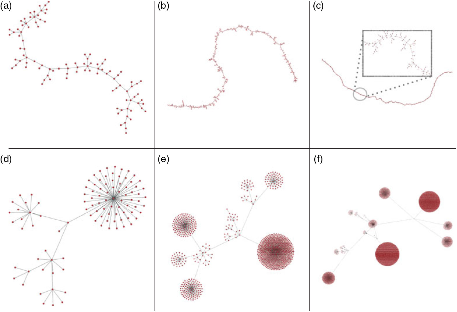
Figure 1: Networks generated by simulating the NRRW, starting with a single node with a self-loop with step parameters
 $s = 1$
(a–c) and
$s = 1$
(a–c) and
 $s = 2$
(d–f) for different stopping times
$s = 2$
(d–f) for different stopping times
 $t =
s(N - 1)$
, with
$t =
s(N - 1)$
, with
 $N = 10^2$
(a, d),
$N = 10^2$
(a, d),
 $N = 10^3$
(b, e), and
$N = 10^3$
(b, e), and
 $N = 10^4$
(c, f).
$N = 10^4$
(c, f).
Interestingly, the NRRW can be analysed from two different perspectives: those of the walker and the network. From the walker’s perspective, a fundamental question concerns the dichotomy between transience and recurrence [Reference Angel, Crawford and Kozma2,Reference Campanino and Petritis4,Reference Dembo, Huang and Sidoravicius6,Reference Disertori, Sabot and Tarrès7,Reference Hoffman, Johnson and Junge9]. Will NRRW give rise to transient or recurrent random walks? From the network perspective, a fundamental question is the dichotomy between a heavy tail and exponential tail degree distribution. What kinds of degrees will NRRW generate? Given the mutual dependence between walker and network, the two perspectives are fundamentally intertwined.
Indeed, Theorem 1 illustrates this close relationship between walker and network properties, establishing that for
 ${s}=1$
the random walk is transient and the node degree is upper-bounded by an exponential distribution. Interestingly, these observations on the walker and the network emerge jointly from the model dynamics, without one being the cause of the other! For s even we show that the walker is recurrent and the degrees of non-leaf nodes are bounded from below by a power law distribution with exponent decreasing in s. Moreover, for s even we also provide a lower bound for the fraction of leaves in the network, and for
${s}=1$
the random walk is transient and the node degree is upper-bounded by an exponential distribution. Interestingly, these observations on the walker and the network emerge jointly from the model dynamics, without one being the cause of the other! For s even we show that the walker is recurrent and the degrees of non-leaf nodes are bounded from below by a power law distribution with exponent decreasing in s. Moreover, for s even we also provide a lower bound for the fraction of leaves in the network, and for
 ${s}=2$
our bound implies that the fraction of leaves goes to one as the network size goes to infinity.
${s}=2$
our bound implies that the fraction of leaves goes to one as the network size goes to infinity.
Why is the parity of s so fundamental? To help build intuition, consider
 $s=1$
. In this case, the walker can move to the node just added and connect a new node to it, pushing the network away from its initial position. For
$s=1$
. In this case, the walker can move to the node just added and connect a new node to it, pushing the network away from its initial position. For
 $s=2$
, the walker can never connect a new node to the node just added, and it will necessarily step back if it moves to the node just added. These two observations – the runaway effect and bouncing-back effect, respectively – play a major role in the dynamics of NRRW, as discussed below.
$s=2$
, the walker can never connect a new node to the node just added, and it will necessarily step back if it moves to the node just added. These two observations – the runaway effect and bouncing-back effect, respectively – play a major role in the dynamics of NRRW, as discussed below.
Finally, various properties of networks generated by NRRW were first observed by means of extensive numerical simulations [Reference Amorim, Figueiredo, Iacobelli, Neglia and Cherifi1], such as the dichotomy in the degrees and distances as a function of the parity of s. In this paper we provide rigorous theoretical treatment for some of the results first observed empirically. In particular, this work makes the following theoretical contributions.
For
 ${s}=1$
the random walk is transient and the degree of a node is bounded above by an exponential distribution (Theorem 1 and Corollary 1, both in Section 3).
${s}=1$
the random walk is transient and the degree of a node is bounded above by an exponential distribution (Theorem 1 and Corollary 1, both in Section 3).For s even the random walk is recurrent and the degree of a non-leaf node is bounded below by a power law distribution with an exponent that depends on s (Theorem 2 and Proposition 1, respectively).
For s even the fraction of leaf nodes is asymptotically lower-bounded by a function that depends on s and is always greater than 2/3 (Theorem 3 and Corollary 4, respectively).

While results for s even are more general and do not strongly depend on the value for s, results for s odd are limited to the case
 ${s}=1$
. Unfortunately, the proof technique used in establishing results for
${s}=1$
. Unfortunately, the proof technique used in establishing results for
 ${s}=1$
does not generalize for other odd values of s. However, simulation results [Reference Amorim, Figueiredo, Iacobelli, Neglia and Cherifi1], as well as recent theoretical results on a similar model (see the discussion in Section 5), strongly indicate that similar theoretical results should hold for all s odd.
${s}=1$
does not generalize for other odd values of s. However, simulation results [Reference Amorim, Figueiredo, Iacobelli, Neglia and Cherifi1], as well as recent theoretical results on a similar model (see the discussion in Section 5), strongly indicate that similar theoretical results should hold for all s odd.
It is important to note the difference between the commonly used network degree distribution and the distribution of the degree of a node, used in this work. While the former refers to the degree of a node chosen uniformly at random at time t, the latter refers to the degree of a fixed node at time t. While the two notions are related, we refrain from further discussion and adopt the latter for simplicity and tractability (and purposely avoid using the expression degree distribution).
The remainder of the paper is organized as follows. Section 2 presents the model and the notation. Results for
 ${s}=1$
are presented in Section 3, while results for s even are presented in Section 4. Finally, Section 5 concludes the paper with a brief discussion and outlook.
${s}=1$
are presented in Section 3, while results for s even are presented in Section 4. Finally, Section 5 concludes the paper with a brief discussion and outlook.
2. The model
The no restart random walk (NRRW) model consists of a random walk moving on a graph that itself grows over time. At every discrete time
 $t>0$
, the random walk takes a step in the current graph (i.e. it chooses a neighbour uniformly at random). After exactly s steps, a new node with degree one (i.e. a leaf node) joins the graph, and is attached to the node currently occupied by the walker (we assume that the attachment of a new node takes zero time).
$t>0$
, the random walk takes a step in the current graph (i.e. it chooses a neighbour uniformly at random). After exactly s steps, a new node with degree one (i.e. a leaf node) joins the graph, and is attached to the node currently occupied by the walker (we assume that the attachment of a new node takes zero time).
Our stochastic process is specified by the pair
 $\{G^{s}_t, W_t\}_{t\geq 0}$
, with
$\{G^{s}_t, W_t\}_{t\geq 0}$
, with
 $((G_0, w_0))$
denoting its initial state where
$((G_0, w_0))$
denoting its initial state where
 $G_0 = (V_0,E_0)$
is an undirected graph with finite node and edge sets
$G_0 = (V_0,E_0)$
is an undirected graph with finite node and edge sets
 $V_0$
and
$V_0$
and
 $E_0$
, respectively, and
$E_0$
, respectively, and
 $w_0 \in V_0$
is the initial position of the random walker. We assume nodes in
$w_0 \in V_0$
is the initial position of the random walker. We assume nodes in
 $V_0$
are labelled with negative numbers, and we let
$V_0$
are labelled with negative numbers, and we let
 ${\mathit{r}}=w_0$
denote the root of our process. New nodes added later are labelled with positive consecutive numbers.
${\mathit{r}}=w_0$
denote the root of our process. New nodes added later are labelled with positive consecutive numbers.
We let
 $G^{s}_t$
denote the graph process resulting at time t from the NRRW with step parameter s:
$G^{s}_t$
denote the graph process resulting at time t from the NRRW with step parameter s:
 $G^{s}_t$
is an undirected graph on the node set
$G^{s}_t$
is an undirected graph on the node set
 $V_t = V_0 \cup \{j , 1\leq j \leq \lfloor t/s \rfloor \}$
, where j is the label of the node added at time j s. We let
$V_t = V_0 \cup \{j , 1\leq j \leq \lfloor t/s \rfloor \}$
, where j is the label of the node added at time j s. We let
 $W_t \in V_t$
denote the position of the walker at time t, and we consider a symmetric random walk, which chooses its next step uniformly at random among the neighbours of its current position. Note that the graph only changes at times
$W_t \in V_t$
denote the position of the walker at time t, and we consider a symmetric random walk, which chooses its next step uniformly at random among the neighbours of its current position. Note that the graph only changes at times
 $t= k {s}$
, for every integer
$t= k {s}$
, for every integer
 $k>0$
, while it does not change in the time intervals
$k>0$
, while it does not change in the time intervals
 $k{s} < t < (k+1){s}$
. Also, since a new node is connected through a single edge, the model adds trees to the initial graph
$k{s} < t < (k+1){s}$
. Also, since a new node is connected through a single edge, the model adds trees to the initial graph
 $G_0$
.
$G_0$
.
The stochastic process
 $\{G^{s}_t, W_t\}_{t\geq 0}$
is always transient: any given graph is observed at most s consecutive steps. Nevertheless, we can define transience and recurrence of the random walk
$\{G^{s}_t, W_t\}_{t\geq 0}$
is always transient: any given graph is observed at most s consecutive steps. Nevertheless, we can define transience and recurrence of the random walk
 $W_t$
in a similar way to a random walk on a static graph. The walker is recurrent (resp. transient) if it visits any node an infinite number of times with probability 1 (resp. 0).
$W_t$
in a similar way to a random walk on a static graph. The walker is recurrent (resp. transient) if it visits any node an infinite number of times with probability 1 (resp. 0).
3. NRRW with step parameter
${s}=1$

Recall that when
 ${s}=1$
, after every walker step a new leaf node is added to the graph. Figure 1(a–c) indicates that in this scenario nodes have small degree (relative to the number of nodes) and the tree grows in depth as the number of nodes increases. More substantial empirical evidence of this phenomenon is provided in [Reference Amorim, Figueiredo, Iacobelli, Neglia and Cherifi1]. This suggests that the random walk is extending the tree to lower depths, never to return to the initial graph
${s}=1$
, after every walker step a new leaf node is added to the graph. Figure 1(a–c) indicates that in this scenario nodes have small degree (relative to the number of nodes) and the tree grows in depth as the number of nodes increases. More substantial empirical evidence of this phenomenon is provided in [Reference Amorim, Figueiredo, Iacobelli, Neglia and Cherifi1]. This suggests that the random walk is extending the tree to lower depths, never to return to the initial graph
 $G_0$
. In other words, the random walk is transient and visits each node in the tree a relatively small number of times, with high probability. The following theorem captures this intuition.
$G_0$
. In other words, the random walk is transient and visits each node in the tree a relatively small number of times, with high probability. The following theorem captures this intuition.
Theorem 1. In the NRRW model with
 $$s=1$$
, for any initial configuration
$$s=1$$
, for any initial configuration
 $$\{G_0, x_0\}$$
with
$$\{G_0, x_0\}$$
with
 $$G_0$$
finite, the random walk is transient. Furthermore, if
$$G_0$$
finite, the random walk is transient. Furthermore, if
 $$J_{G_0}=\sum_{t=0}^\infty {\bf 1}(W_t\in V(G_0))$$
denotes the number of visits to the initial graph, there exist constants
$$J_{G_0}=\sum_{t=0}^\infty {\bf 1}(W_t\in V(G_0))$$
denotes the number of visits to the initial graph, there exist constants
 $$a,b>0$$
such that, for all
$$a,b>0$$
such that, for all
 $$k>0$$
,
$$k>0$$
,
 $$\mathbb{P}(J_{G_0}\geq k )\leq a{\mathrm{e}}^{-bk} .$$
A similar theorem considering the case in which the initial graph
 $G_0$
is a single node has appeared in [Reference Amorim, Figueiredo, Iacobelli, Neglia and Cherifi1]; here, we generalize this prior result to any initial graph
$G_0$
is a single node has appeared in [Reference Amorim, Figueiredo, Iacobelli, Neglia and Cherifi1]; here, we generalize this prior result to any initial graph
 $G_0$
.
$G_0$
.
Proof. We begin by proving that the random walk is transient.
Let
 $\tau^-_1(x_0)\,:\!=\inf\{t>0\colon W_t \not \in V(G_0)\}$
be the first time the random walk visits a node not in
$\tau^-_1(x_0)\,:\!=\inf\{t>0\colon W_t \not \in V(G_0)\}$
be the first time the random walk visits a node not in
 $G_0$
starting from
$G_0$
starting from
 $x_0$
(in what follows we usually omit the dependence on
$x_0$
(in what follows we usually omit the dependence on
 $x_0$
).
$x_0$
).
It is not difficult to see that
 $${\mathbb{P}}(\tau _1^ - > m) \le {(1 - \frac{1}{{\Delta ({G_0}) + 1}})^m} \le {{\rm{e}}^{ - m/\Delta ({G_0}) + 1}},$$
where
 $$\Delta(G_0)$$
denotes the maximal degree in
$$\Delta(G_0)$$
denotes the maximal degree in
 $$G_0$$
. Thus, in particular,
$$G_0$$
. Thus, in particular,
 $$\tau^-_1$$
is finite almost surely and this holds for any finite graph
$$\tau^-_1$$
is finite almost surely and this holds for any finite graph
 $$G_0$$
and any initial position
$$G_0$$
and any initial position
 $$x_0 \in V(G_0)$$
of the walker. We call this time the beginning of the first excursion and we let
$$x_0 \in V(G_0)$$
of the walker. We call this time the beginning of the first excursion and we let
 $$v_1=W_{\tau^-_1}$$
denote the node where the excursion begins. We also define
$$v_1=W_{\tau^-_1}$$
denote the node where the excursion begins. We also define
 $$\tau _1^ + {\mkern 1mu} : = \inf \{ t > \tau _1^ - :{W_t} \in V({G_0})\} ,$$
the first time the random walk comes back to
 $$G_0$$
, which denotes the end of the first excursion. Similarly, we define the beginning and end of the ith excursion as
$$G_0$$
, which denotes the end of the first excursion. Similarly, we define the beginning and end of the ith excursion as
 $$
\begin{align*}
\tau^-_i &\,:\!= \begin{cases}
\inf \{t> \tau^+_{i-1}\colon W_t \not \in V(G_0)\} & \text{if $\tau^+_{i-1}<+\infty$} ,
\\
+ \infty & \text{otherwise} ,
\end{cases}
\\*
\tau^+_i &\,:\!= \begin{cases}
\inf \{t> \tau^-_{i} \colon W_t \in V(G_0)\} & \text{if $\tau^-_{i}<+\infty$} ,
\\
+ \infty & \text{otherwise} .
\end{cases}
\end{align*}
$$
$$
\begin{align*}
\tau^-_i &\,:\!= \begin{cases}
\inf \{t> \tau^+_{i-1}\colon W_t \not \in V(G_0)\} & \text{if $\tau^+_{i-1}<+\infty$} ,
\\
+ \infty & \text{otherwise} ,
\end{cases}
\\*
\tau^+_i &\,:\!= \begin{cases}
\inf \{t> \tau^-_{i} \colon W_t \in V(G_0)\} & \text{if $\tau^-_{i}<+\infty$} ,
\\
+ \infty & \text{otherwise} .
\end{cases}
\end{align*}
$$
Note that if the ith excursion ends after a finite time, i.e. if
 $$\tau^+_{i}<+ \infty$$
, then the walker will almost surely spend a finite time visiting nodes in
$$\tau^+_{i}<+ \infty$$
, then the walker will almost surely spend a finite time visiting nodes in
 $$G_0$$
, before starting the
$$G_0$$
, before starting the
 $$(i+1)$$
th excursion. This is due to the fact that new nodes may be added to nodes in
$$(i+1)$$
th excursion. This is due to the fact that new nodes may be added to nodes in
 $$G_0$$
and they increase the chance of the walker leaving
$$G_0$$
and they increase the chance of the walker leaving
 $$G_0$$
. Formally,
$$G_0$$
. Formally,
 $$\tau_{i+1}^- - \tau_{i}^+ \le \tau_{1}^- (W_{\tau_i^+})$$
.
$$\tau_{i+1}^- - \tau_{i}^+ \le \tau_{1}^- (W_{\tau_i^+})$$
.
While the walker spends a finite time in
 $$G_0$$
between two excursions, we prove that it may never come back from an excursion, that is, for each i,
$$G_0$$
between two excursions, we prove that it may never come back from an excursion, that is, for each i,
 $$\mathbb{P}(\tau^+_i = +\infty \mid \tau^-_i < + \infty)>0$$
. We consider that the walker starts the ith excursion from a leaf, due to the fact that starting an excursion in a node with higher degree can only increase the duration of an excursion.
$$\mathbb{P}(\tau^+_i = +\infty \mid \tau^-_i < + \infty)>0$$
. We consider that the walker starts the ith excursion from a leaf, due to the fact that starting an excursion in a node with higher degree can only increase the duration of an excursion.
Let
 $$X_{n}= d(W_{\tau^-_i + n}, G_0)$$
for
$$X_{n}= d(W_{\tau^-_i + n}, G_0)$$
for
 $$0 \le n \le \tau^+_i - \tau^-_i$$
denote the graph distance between the position of the walker and the initial graph
$$0 \le n \le \tau^+_i - \tau^-_i$$
denote the graph distance between the position of the walker and the initial graph
 $$G_0$$
after n steps of the ith excursion. We call the process
$$G_0$$
after n steps of the ith excursion. We call the process
 $$\{X_{n}, n \in \mathbb{Z}_{\ge 0}\}$$
the level process. At any step of the ith excursion the RW is in a node
$$\{X_{n}, n \in \mathbb{Z}_{\ge 0}\}$$
the level process. At any step of the ith excursion the RW is in a node
 $$v_n$$
with at least two edges: the one the RW has arrived from and the new one added as a consequence of the RW’s arrival to that node (recall that for
$$v_n$$
with at least two edges: the one the RW has arrived from and the new one added as a consequence of the RW’s arrival to that node (recall that for
 $${s}=1$$
after every walker step a new node is attached to the graph). We let
$${s}=1$$
after every walker step a new node is attached to the graph). We let
 $$p_{k,h}(n)$$
denote the probability that the level at step
$$p_{k,h}(n)$$
denote the probability that the level at step
 $$n+1$$
is h conditioned on the fact that it is k at step n. Let
$$n+1$$
is h conditioned on the fact that it is k at step n. Let
 $$d_n \ge 2$$
denote the degree of node
$$d_n \ge 2$$
denote the degree of node
 $$v_n$$
, then the RW moves from
$$v_n$$
, then the RW moves from
 $$v_n$$
to a node with a larger level with probability
$$v_n$$
to a node with a larger level with probability
 $${p_{k,k + 1}}(n) = {\rm{(}}{d_n} - 1)/{d_n} \ge {\rm{ }}1/2$$
and with the complementary probability
$${p_{k,k + 1}}(n) = {\rm{(}}{d_n} - 1)/{d_n} \ge {\rm{ }}1/2$$
and with the complementary probability
 $${p_{k,k - 1}}(n) = 1/{d_n} \le {\rm{ }}1/2$$
to a node with smaller level. It is worth mentioning that the nodes’ degrees keep changing due to the arrival of new nodes (edges), and therefore the level process is non-homogeneous (both in time and in space). Moreover, although the notation hides it, the probabilities
$${p_{k,k - 1}}(n) = 1/{d_n} \le {\rm{ }}1/2$$
to a node with smaller level. It is worth mentioning that the nodes’ degrees keep changing due to the arrival of new nodes (edges), and therefore the level process is non-homogeneous (both in time and in space). Moreover, although the notation hides it, the probabilities
 $$p_{k,h}(n)$$
depend on the whole history of the RW until step n.
$$p_{k,h}(n)$$
depend on the whole history of the RW until step n.
We then look at this process every two walker steps, that is, we consider the process
 $${Y_m} \triangle {X_{\tau _i^ - + 2m}}$$
, starting from
$${Y_m} \triangle {X_{\tau _i^ - + 2m}}$$
, starting from
 $$Y_0=1$$
. The two-step level process can be seen as a non-homogeneous ‘lazy’ random walk on
$$Y_0=1$$
. The two-step level process can be seen as a non-homogeneous ‘lazy’ random walk on
 $$\{1,3,5,\ldots\}$$
. The two-step level process will provide a bound to the transition probabilities
$$\{1,3,5,\ldots\}$$
. The two-step level process will provide a bound to the transition probabilities
 $$p_{k,h}(n)$$
that allows a simple coupling with a homogeneous (and biased) random walk. The previous bounds for
$$p_{k,h}(n)$$
that allows a simple coupling with a homogeneous (and biased) random walk. The previous bounds for
 $$X_n$$
immediately lead us to conclude that
$$X_n$$
immediately lead us to conclude that
 $${p_{k,k + 2}}(n) \ge \frac{1}{2}\frac{1}{2} = \frac{1}{4}\quad {\rm{for any level }}k \ge {\rm{1}}$$
and
 $$p_{k,k-2}(n)\le \dfrac{1}{2} \dfrac{1}{2}=\dfrac{1}{4}\quad \text{for k\ge 3.}$$
We can get a tighter bound for
 $$p_{k,k-2}(n)$$
for
$$p_{k,k-2}(n)$$
for
 $$k \geq 3$$
. If the RW is at level
$$k \geq 3$$
. If the RW is at level
 $$k\geq 3$$
, all nodes on the path between its current position and the node where the excursion began have degree at least 2. If it then moves to node v at level
$$k\geq 3$$
, all nodes on the path between its current position and the node where the excursion began have degree at least 2. If it then moves to node v at level
 $$k-1$$
, a new edge is attached to v, whose degree is now at least 3. The probability of moving from v to a node with level
$$k-1$$
, a new edge is attached to v, whose degree is now at least 3. The probability of moving from v to a node with level
 $$k-2$$
is then at most
$$k-2$$
is then at most
 $ 1/3 $
. It then follows that
$ 1/3 $
. It then follows that
 $$p_{k,k-2}(n)\le \dfrac{1}{2} \dfrac{1}{3}=\dfrac{1}{6}\quad\text{for $k\ge 3$.}
$$
$$p_{k,k-2}(n)\le \dfrac{1}{2} \dfrac{1}{3}=\dfrac{1}{6}\quad\text{for $k\ge 3$.}
$$
By a standard coupling argument it is possible to show that
 $$Y_n^* \le_{\textrm{st}} Y_n$$
, where
$$Y_n^* \le_{\textrm{st}} Y_n$$
, where
 $$(Y^*_n)_{n\geq 0}$$
is a homogeneous biased lazy random walk on
$$(Y^*_n)_{n\geq 0}$$
is a homogeneous biased lazy random walk on
 $$\{1,3,5,\ldots\}$$
, starting from
$$\{1,3,5,\ldots\}$$
, starting from
 $$Y_0^*=1$$
, with transition probabilities
$$Y_0^*=1$$
, with transition probabilities
 $p_{k,k + 2}^* = 1/4$
for all
$p_{k,k + 2}^* = 1/4$
for all
 $$k \geq 1$$
and
$$k \geq 1$$
and
 $p^*_{k,k-2}= 1/6$
for
$p^*_{k,k-2}= 1/6$
for
 $$k \geq 3$$
. The homogeneous biased lazy random walk
$$k \geq 3$$
. The homogeneous biased lazy random walk
 $$(Y_n^*)_{n\geq 0}$$
is transient since
$$(Y_n^*)_{n\geq 0}$$
is transient since
 $$p^*_{k,k+2}=1/4 > p^*_{k,k-2}=1/6$$
. Thus, if
$$p^*_{k,k+2}=1/4 > p^*_{k,k-2}=1/6$$
. Thus, if
 $$\eta\,:\!=\inf \{n>0\colon Y^*_n=0\}$$
, it holds that
$$\eta\,:\!=\inf \{n>0\colon Y^*_n=0\}$$
, it holds that
 $$f_0=\mathbb{P}(\eta<+\infty)<1$$
and the coupling ensures that
$$f_0=\mathbb{P}(\eta<+\infty)<1$$
and the coupling ensures that
 $$\mathbb{P}(\tau^+_i<+\infty \mid \tau^-_i < + \infty)\leq f_0<1$$
; this implies that the random walk is transient.
$$\mathbb{P}(\tau^+_i<+\infty \mid \tau^-_i < + \infty)\leq f_0<1$$
; this implies that the random walk is transient.
We now show the second claim. Let N be a random variable counting the number of excursions and let
 $$\{Z_n\}_{n}$$
be a sequence of i.i.d. geometric random variables,
$$\{Z_n\}_{n}$$
be a sequence of i.i.d. geometric random variables,
 $$Z_n \sim \textrm{Geo}(p)$$
with
$$Z_n \sim \textrm{Geo}(p)$$
with
 $$p=(\Delta(G_0)+1)^{-1}$$
, independent of N. Then, it is not difficult to see that the random variable
$$p=(\Delta(G_0)+1)^{-1}$$
, independent of N. Then, it is not difficult to see that the random variable
 $$J_{G_0}$$
is stochastically dominated by
$$J_{G_0}$$
is stochastically dominated by
 $$\sum_{i=1}^N Z_i$$
, that is,
$$\sum_{i=1}^N Z_i$$
, that is,
 $${\mathbb{P}}({J_{{G_0}}} > k) \le {\mathbb{P}}(\sum\limits_{i = 1}^N {{Z_i}} > k).$$
Using the Chernoff bound, together with the fact that the random variable N satisfies
 $$\mathbb{P}(N\geq k) \leq f_0^k$$
, we obtain that, for every
$$\mathbb{P}(N\geq k) \leq f_0^k$$
, we obtain that, for every
 $$t\geq 0$$
sufficiently small (i.e. such that
$$t\geq 0$$
sufficiently small (i.e. such that
 $${\mathrm{e}}^t (1- p ) <1$$
), the following holds:
$${\mathrm{e}}^t (1- p ) <1$$
), the following holds:
 $$
\begin{align*}
\mathbb{P}(J_{G_0}\geq k)&\leq \mathbb{P}\bigg(\sum_{i=1}^N Z_i \geq k\bigg)\\*
& \leq \sum_{m=1}^\infty \mathbb{P}\bigg(\sum_{i=1}^m Z_i \geq k\bigg)f_0^m\\
& \leq {\mathrm{e}}^{-tk} \sum_{m=1}^\infty \prod_{i=1}^m \mathbb{E}({\mathrm{e}}^{tZ_i})f_0^m \\*
&= {\mathrm{e}}^{-tk} \sum_{m=1}^\infty \bigg( \dfrac{pf_0}{{\mathrm{e}}^{-t} -1 + p}\bigg)^m .
\end{align*}
$$
$$
\begin{align*}
\mathbb{P}(J_{G_0}\geq k)&\leq \mathbb{P}\bigg(\sum_{i=1}^N Z_i \geq k\bigg)\\*
& \leq \sum_{m=1}^\infty \mathbb{P}\bigg(\sum_{i=1}^m Z_i \geq k\bigg)f_0^m\\
& \leq {\mathrm{e}}^{-tk} \sum_{m=1}^\infty \prod_{i=1}^m \mathbb{E}({\mathrm{e}}^{tZ_i})f_0^m \\*
&= {\mathrm{e}}^{-tk} \sum_{m=1}^\infty \bigg( \dfrac{pf_0}{{\mathrm{e}}^{-t} -1 + p}\bigg)^m .
\end{align*}
$$
Choosing t sufficiently small such that
 $p{f_0}{\rm{/(}}{{\rm{e}}^{ - t}} - 1 + p) < 1$
, we obtain the claim. □
$p{f_0}{\rm{/(}}{{\rm{e}}^{ - t}} - 1 + p) < 1$
, we obtain the claim. □
Corollary 1. In NRRW with
 $${s}=1$$
, the degree of any node is bounded above by 1 plus a random variable J such that
$${s}=1$$
, the degree of any node is bounded above by 1 plus a random variable J such that
 $$\mathbb{P}(J>k) \leq a \,{\mathrm{e}}^{-bk}$$
, for some constants
$$\mathbb{P}(J>k) \leq a \,{\mathrm{e}}^{-bk}$$
, for some constants
 $$a,b>0$$
.
$$a,b>0$$
.
This follows because when
 $${s}=1$$
a new node is added after every walker step. Thus, the degree of a node is equal to 1 plus the number of visits the random walk makes to the node. If we consider a node v added at time t we can apply Theorem 1, setting
$${s}=1$$
a new node is added after every walker step. Thus, the degree of a node is equal to 1 plus the number of visits the random walk makes to the node. If we consider a node v added at time t we can apply Theorem 1, setting
 $$G_0=G_t$$
and
$$G_0=G_t$$
and
 $$W_0=v$$
, and obtain that the number of visits to node v will be smaller than the visits to
$$W_0=v$$
, and obtain that the number of visits to node v will be smaller than the visits to
 $$G_t$$
.
$$G_t$$
.
4. NRRW with even step parameter
This section investigates the behaviour of NRRW for s even, highlighting some fundamental differences with the case
 $${s}=1$$
. In particular, we prove the following results.
$${s}=1$$
. In particular, we prove the following results.
The random walk is recurrent, i.e. it visits every node of the graph infinitely often almost surely.
The degree of any non-leaf node is lower-bounded by a power law.
The fraction of leaves is asymptotically lower-bounded by a constant that depends on s. In particular, for
$${s}=2$$
the fraction of leaves goes to 1 while for any s it is greater than 2/3.

An important difference between s even and s odd is that two new consecutive nodes can be connected to the same node when s is even, which is not possible when
 $$s=1$$
(or s odd, in general). Moreover, the more nodes are consecutively connected to node i, the higher is the probability that the next node will also connect to i. This produces what we call the bouncing-back effect, which increases the probability of returning to i after an even number of steps. Assume, for example, that
$$s=1$$
(or s odd, in general). Moreover, the more nodes are consecutively connected to node i, the higher is the probability that the next node will also connect to i. This produces what we call the bouncing-back effect, which increases the probability of returning to i after an even number of steps. Assume, for example, that
 $${s}=2$$
and that M new nodes have been consecutively connected to node i. All the M newly added nodes are leaves, and therefore, as soon as the walker visits any one of them (which happens with probability proportional to M), it must return to node i in the next step, thus adding a further leaf to i. The bouncing-back effect is the fundamental difference between the dynamics of s even and odd. Finally, we note that this effect is related to ‘cumulative advantage’ or ‘rich-get-richer’ effects, since the more resources an agent has (leaves of a node, in our case) the easier it becomes to accumulate further resources.
$${s}=2$$
and that M new nodes have been consecutively connected to node i. All the M newly added nodes are leaves, and therefore, as soon as the walker visits any one of them (which happens with probability proportional to M), it must return to node i in the next step, thus adding a further leaf to i. The bouncing-back effect is the fundamental difference between the dynamics of s even and odd. Finally, we note that this effect is related to ‘cumulative advantage’ or ‘rich-get-richer’ effects, since the more resources an agent has (leaves of a node, in our case) the easier it becomes to accumulate further resources.
The analysis that follows assumes that the initial network
 $$G_0$$
is given by a single node with a self-loop, denoted by
$$G_0$$
is given by a single node with a self-loop, denoted by
 $${\mathit{r}}=w_0$$
, the root of the process. The results obtained can be generalized to any arbitrary initial network
$${\mathit{r}}=w_0$$
, the root of the process. The results obtained can be generalized to any arbitrary initial network
 $$\{G_0, W_0\}$$
, where
$$\{G_0, W_0\}$$
, where
 $$G_0$$
is a finite connected and non-bipartite graph.
$$G_0$$
is a finite connected and non-bipartite graph.
4.1. Degree of nodes with s even
Corollary 1 determines that when
 $${s}=1$$
the degree of every non-leaf node (i.e. nodes having degree greater than one) is bounded from above by a geometric distribution. In sharp contrast, we show that for every s even the degree of non-leaf nodes is bounded from below by a power law distribution whose exponent depends on s. The dichotomy in NRRW between the exponential tail and heavy tail for the degree of non-leaf nodes for s odd and s even has been empirically observed in simulations [Reference Amorim, Figueiredo, Iacobelli, Neglia and Cherifi1].
$${s}=1$$
the degree of every non-leaf node (i.e. nodes having degree greater than one) is bounded from above by a geometric distribution. In sharp contrast, we show that for every s even the degree of non-leaf nodes is bounded from below by a power law distribution whose exponent depends on s. The dichotomy in NRRW between the exponential tail and heavy tail for the degree of non-leaf nodes for s odd and s even has been empirically observed in simulations [Reference Amorim, Figueiredo, Iacobelli, Neglia and Cherifi1].
Proposition 1. Let s be even and assume that
 $$T_j$$
is the first time a leaf is connected to node j. Then, for every time
$$T_j$$
is the first time a leaf is connected to node j. Then, for every time
 $$t \geq T_j$$
and for every
$$t \geq T_j$$
and for every
 $$k \in \{ 1, \ldots ,[t - {T_j}/s] + 1\}$$
, we have that
$$k \in \{ 1, \ldots ,[t - {T_j}/s] + 1\}$$
, we have that
 $$
\begin{alignat*}{3}
&\mathbb{P}(d_{t}(j)\geq k+1 \mid T_j < \infty) \geq
k^{-{s}/2} &\quad & \text{if $j \neq $ root} , \\
&\mathbb{P}(d_{t}(j)\geq k+2) \geq \bigg( \dfrac{k(k+1)}{2}\bigg)^{-{s}/2} && \text{if $j = $ root} ,
\end{alignat*}
$$
$$
\begin{alignat*}{3}
&\mathbb{P}(d_{t}(j)\geq k+1 \mid T_j < \infty) \geq
k^{-{s}/2} &\quad & \text{if $j \neq $ root} , \\
&\mathbb{P}(d_{t}(j)\geq k+2) \geq \bigg( \dfrac{k(k+1)}{2}\bigg)^{-{s}/2} && \text{if $j = $ root} ,
\end{alignat*}
$$
where
 $$d_t(j)$$
denotes the degree of node j at time t.
$$d_t(j)$$
denotes the degree of node j at time t.
Proof. To prove the claim, we compute the degree of a node in a much simpler process. This simpler process starts at time 0 with a 3-node graph made by a node c that has exactly one child (leaf) and one parent and the random walk placed on node c. If at any step the random walk chooses the parent node, the process stops. Otherwise, after s steps the random walk adds a new leaf node. Note that since s is even, this simple process will grow a star. The star stops growing when the random walk steps into the parent node. Figure 2 illustrates this simple star growing process.

Figure 2: Configurations from the star growing process used to bound the degree of non-leaf nodes in NRRW with s even (Proposition 1). The dashed edge represents the edge to the parent node, solid edges represent edge to leaves, and the red (square) node represents the walker position at the corresponding time.
At time
 $$t>0$$
the random walk can have added at most ˪t/s˩ nodes to c. In particular, it adds one node if for s consecutive steps, it selects a child of c (this happens with probability
$$t>0$$
the random walk can have added at most ˪t/s˩ nodes to c. In particular, it adds one node if for s consecutive steps, it selects a child of c (this happens with probability
 $$i/(i+1)$$
if i is the current degree of node c) and then steps back to c. It follows that the probability that the degree of node c at time t (we denote it by
$$i/(i+1)$$
if i is the current degree of node c) and then steps back to c. It follows that the probability that the degree of node c at time t (we denote it by
 $$d_t(c)$$
) is at least
$$d_t(c)$$
) is at least
 $$k+1$$
for
$$k+1$$
for
 $$k \in \{ 1, \ldots ,\,\,[t/s] + 1\} $$
is equal to
$$k \in \{ 1, \ldots ,\,\,[t/s] + 1\} $$
is equal to
 $${\mathbb{P}}({d_t}(c) \ge k + 1) = \prod\limits_{i = 1}^{k - 1} ( \frac{i}{{i + 1}}{)^{s/2}} = {(\frac{1}{k})^{s/2}},$$
with the usual convention that
 $$\prod\limits_{i = 1}^0 {{{(i/(i + 1))}^{s/2}}} = 1$$
.
$$\prod\limits_{i = 1}^0 {{{(i/(i + 1))}^{s/2}}} = 1$$
.
Let j be an arbitrary node of the graph generated by the NRRW model with even step parameter s and assume that
 $$T_j < \infty$$
(recall that
$$T_j < \infty$$
(recall that
 $$T_j$$
is the first time a new node is connected to node j). Let us first consider the case in which j is different from the root. At time
$$T_j$$
is the first time a new node is connected to node j). Let us first consider the case in which j is different from the root. At time
 $$T_j$$
node j has exactly two neighbours: a leaf and a parent. Thus, at this point in time, the dynamics of the NRRW model is similar to that of the simple star growing process described above.
$$T_j$$
node j has exactly two neighbours: a leaf and a parent. Thus, at this point in time, the dynamics of the NRRW model is similar to that of the simple star growing process described above.
In particular, the probability that, at time
 $$t \geq T_j$$
, the degree
$$t \geq T_j$$
, the degree
 $$d_{t}(j)$$
is larger than
$$d_{t}(j)$$
is larger than
 $$k+1$$
for
$$k+1$$
for
 $$k \in \{ 1, \ldots ,[(t - {T_j})/s] + 1\} $$
is greater than the probability that the corresponding probability for the simple star, because the new nodes can be added to j without being consecutive, and in particular, nodes can still be added after the random walk steps on to the parent node.
$$k \in \{ 1, \ldots ,[(t - {T_j})/s] + 1\} $$
is greater than the probability that the corresponding probability for the simple star, because the new nodes can be added to j without being consecutive, and in particular, nodes can still be added after the random walk steps on to the parent node.
In the case when j is the root (
 $$j={\mathit{r}}$$
), we have
$$j={\mathit{r}}$$
), we have
 $$T_j={s}$$
. Moreover, we can treat the self-loop at the root as the edge leading to the parent node. In order to bound the root degree, we consider a slight variation of the star growing process since the initial configuration has a self-loop. Consequently, the probability that the walker takes the leaf node in the first step equals 1/3 (rather than 1/2) and the probability that it takes the self-loop in the first step is 2/3. If
$$T_j={s}$$
. Moreover, we can treat the self-loop at the root as the edge leading to the parent node. In order to bound the root degree, we consider a slight variation of the star growing process since the initial configuration has a self-loop. Consequently, the probability that the walker takes the leaf node in the first step equals 1/3 (rather than 1/2) and the probability that it takes the self-loop in the first step is 2/3. If
 $$c_{\mathit{r}}$$
denotes the centre node of this variant of the star growing process, similarly to the previous case, for
$$c_{\mathit{r}}$$
denotes the centre node of this variant of the star growing process, similarly to the previous case, for
 $$k \in \{ 1, \ldots ,[t/s] + 1\} $$
, we have
$$k \in \{ 1, \ldots ,[t/s] + 1\} $$
, we have
 $$P({d_t}({c_r}) \ge k + 2) = \prod\limits_{i = 1}^{k - 1} ( \frac{i}{{i + 2}}{)^{s/2}} = {(\frac{2}{{k(k + 1)}})^{s/2}}.$$
and then the lower bound for the degree
 $$d_t(r)$$
is derived via the same reasoning. □
$$d_t(r)$$
is derived via the same reasoning. □
Despite the presence of the bouncing-back effect, it is worth noting that the random walk will not get stuck adding consecutive leaves to a node, and it will eventually stop bouncing. In particular, we show that for any s even, the probability of bouncing back k times goes to zero at least as fast as
 $$k^{-1/2}$$
.
$$k^{-1/2}$$
.
Lemma 1. Let s be even,
 $$t_0 \in 2\mathbb{Z}_{\geq 0}$$
and
$$t_0 \in 2\mathbb{Z}_{\geq 0}$$
and
 $$t_0 \ge s$$
, and i a node of the graph. Then, for all
$$t_0 \ge s$$
, and i a node of the graph. Then, for all
 $$k\geq 1$$
, we have
$$k\geq 1$$
, we have
 $${\mathbb{P}}({{\rm{W}}_{{t_0} + 2}} = i,{{\rm{W}}_{{t_0} + 4}} = i, \ldots ,{{\rm{W}}_{{t_0} + 2k}} = i\mid {{\rm{W}}_{{t_0}}} = i) \le \left\{ {\begin{array}{*{20}{l}}
{2\frac{{\sqrt {{d_{{t_0}}}(i) - 1} }}{{\sqrt {{d_{{t_0}}}(i) + k - 1} }}}&{{\rm{if }}{d_{{{\rm{t}}_{\rm{0}}}}}({\rm{i}}) \ge {\rm{2}},}\\
{\frac{1}{{\sqrt k }}}&{{\rm{if }}{d_{{{\rm{t}}_{\rm{0}}}}}({\rm{i}}){\rm{ = 1}},}
\end{array}} \right.$$
$${\mathbb{P}}({{\rm{W}}_{{t_0} + 2}} = i,{{\rm{W}}_{{t_0} + 4}} = i, \ldots ,{{\rm{W}}_{{t_0} + 2k}} = i\mid {{\rm{W}}_{{t_0}}} = i) \le \left\{ {\begin{array}{*{20}{l}}
{2\frac{{\sqrt {{d_{{t_0}}}(i) - 1} }}{{\sqrt {{d_{{t_0}}}(i) + k - 1} }}}&{{\rm{if }}{d_{{{\rm{t}}_{\rm{0}}}}}({\rm{i}}) \ge {\rm{2}},}\\
{\frac{1}{{\sqrt k }}}&{{\rm{if }}{d_{{{\rm{t}}_{\rm{0}}}}}({\rm{i}}){\rm{ = 1}},}
\end{array}} \right.$$
where
 $$d_{t_0} (i)$$
is the degree of node i at time
$$d_{t_0} (i)$$
is the degree of node i at time
 $$t_0$$
.
$$t_0$$
.
Proof. Let
 $$\mathcal{N}_{t_0} (i)$$
denote the set of neighbouring nodes of i at time
$$\mathcal{N}_{t_0} (i)$$
denote the set of neighbouring nodes of i at time
 $$t_0$$
. The probability that the walker returns to i at time
$$t_0$$
. The probability that the walker returns to i at time
 $$t_0 + 2$$
given that
$$t_0 + 2$$
given that
 $${\mathrm{W}}_{t_0}=i$$
is equal to
$${\mathrm{W}}_{t_0}=i$$
is equal to
 $$B_{t_0}(i)/d_{t_0}(i)$$
, where
$$B_{t_0}(i)/d_{t_0}(i)$$
, where
 $${B_{{t_0}}}(i) = \left\{ {\begin{array}{*{20}{l}}
{\sum\limits_{j \in {\rm{ }}{{\mathcal{N}}_{{t_0}}}(i)} {\frac{1}{{{d_{{t_0}}}({\mkern 1mu} j)}}} }&{{\rm{if }}i \ne r,}\\
{[9pt]\sum\limits_{j \in {\rm{ }}{{\mathcal{N}}_{{t_0}}}(r)\backslash \{ r\} } {\frac{1}{{{d_{{t_0}}}({\mkern 1mu} j)}}} + \frac{4}{{{d_{{t_0}}}(r)}}}&{{\rm{if }}i{\rm{ = }}r.}
\end{array}} \right.$$
$${B_{{t_0}}}(i) = \left\{ {\begin{array}{*{20}{l}}
{\sum\limits_{j \in {\rm{ }}{{\mathcal{N}}_{{t_0}}}(i)} {\frac{1}{{{d_{{t_0}}}({\mkern 1mu} j)}}} }&{{\rm{if }}i \ne r,}\\
{[9pt]\sum\limits_{j \in {\rm{ }}{{\mathcal{N}}_{{t_0}}}(r)\backslash \{ r\} } {\frac{1}{{{d_{{t_0}}}({\mkern 1mu} j)}}} + \frac{4}{{{d_{{t_0}}}(r)}}}&{{\rm{if }}i{\rm{ = }}r.}
\end{array}} \right.$$
If, after coming back m consecutive times to i, we have added
 $$h\le m$$
nodes (necessarily to i), then
$$h\le m$$
nodes (necessarily to i), then
 $$B_{t_0+2m} (i)\le B_{t_0} (i)+h$$
, where the equality holds for
$$B_{t_0+2m} (i)\le B_{t_0} (i)+h$$
, where the equality holds for
 $$i \neq {\mathit{r}}$$
. But then, because
$$i \neq {\mathit{r}}$$
. But then, because
 $$B_t(i)/d_t(i)$$
is smaller than 1, we obtain
$$B_t(i)/d_t(i)$$
is smaller than 1, we obtain
 $$\dfrac{B_{t_0+2m}(i)}{d_{t_0+2m}(i)} \le \dfrac{B_{t_0} (i)+h}{d_{t_0} (i)+h} \le \dfrac{B_{t_0} (i)+m}{d_{t_0} (i)+m} {.} $$
It then follows that
 $$\begin{array}{l}
{\mathbb{P}}({{\rm{W}}_{{t_0} + 2}} = i,{{\rm{W}}_{{t_0} + 4}} = i, \ldots ,{{\rm{W}}_{{t_0} + 2k}} = i\mid {{\rm{W}}_{{t_0}}} = i)\\
\qquad = \frac{{{B_{{t_0}}}(i)}}{{{d_{{t_0}}}(i)}} \cdot \frac{{{B_{{t_0} + 2}}(i)}}{{{d_{{t_0} + 2}}(i)}} \cdot \ldots \cdot \frac{{{B_{{t_0} + 2(k - 1)}}(i)}}{{{d_{{t_0} + 2(k - 1)}}(i)}}\\
\qquad \le \frac{{{B_{{t_0}}}(i)}}{{{d_{{t_0}}}(i)}} \cdot \frac{{{B_{{t_0}}}(i) + 1}}{{{d_{{t_0}}}(i) + 1}} \cdot \ldots \cdot \frac{{{B_{{t_0}}}(i) + (k - 1)}}{{{d_{{t_0}}}(i) + (k - 1)}}.
\end{array}$$
$$\begin{array}{l}
{\mathbb{P}}({{\rm{W}}_{{t_0} + 2}} = i,{{\rm{W}}_{{t_0} + 4}} = i, \ldots ,{{\rm{W}}_{{t_0} + 2k}} = i\mid {{\rm{W}}_{{t_0}}} = i)\\
\qquad = \frac{{{B_{{t_0}}}(i)}}{{{d_{{t_0}}}(i)}} \cdot \frac{{{B_{{t_0} + 2}}(i)}}{{{d_{{t_0} + 2}}(i)}} \cdot \ldots \cdot \frac{{{B_{{t_0} + 2(k - 1)}}(i)}}{{{d_{{t_0} + 2(k - 1)}}(i)}}\\
\qquad \le \frac{{{B_{{t_0}}}(i)}}{{{d_{{t_0}}}(i)}} \cdot \frac{{{B_{{t_0}}}(i) + 1}}{{{d_{{t_0}}}(i) + 1}} \cdot \ldots \cdot \frac{{{B_{{t_0}}}(i) + (k - 1)}}{{{d_{{t_0}}}(i) + (k - 1)}}.
\end{array}$$
We observe that equality holds, for
 $$i\neq {\mathit{r}}$$
, when
$$i\neq {\mathit{r}}$$
, when
 $${s}=2$$
and the walker indeed adds a new leaf every time it bounces back to node i. Also, we have that
$${s}=2$$
and the walker indeed adds a new leaf every time it bounces back to node i. Also, we have that
 $$B_{t_0} (i)\leq d_{t_0} (i) - 1/2$$
, and this holds regardless of whether or not
$$B_{t_0} (i)\leq d_{t_0} (i) - 1/2$$
, and this holds regardless of whether or not
 $$i={\mathit{r}}$$
. For
$$i={\mathit{r}}$$
. For
 $$i\neq {\mathit{r}}$$
, the inequality
$$i\neq {\mathit{r}}$$
, the inequality
 $$B_{t_0} (i)\leq d_{t_0} (i) - 1/2$$
follows from the observation that if the random walk is in i at time
$$B_{t_0} (i)\leq d_{t_0} (i) - 1/2$$
follows from the observation that if the random walk is in i at time
 $$t_0$$
, the node i has at least one neighbour which is not a leaf (it might be the only one) and therefore the latter will have degree at least 2. Hence,
$$t_0$$
, the node i has at least one neighbour which is not a leaf (it might be the only one) and therefore the latter will have degree at least 2. Hence,
 $$\sum_{j \in \mathcal{N}_{t_0} (i)}
\dfrac{1}{d_{t_0} (j)} \leq d_{t_0} (i) -1 + \dfrac{1}{2} = d_{t_0} (i) - \dfrac{1}{2}.$$
$$\sum_{j \in \mathcal{N}_{t_0} (i)}
\dfrac{1}{d_{t_0} (j)} \leq d_{t_0} (i) -1 + \dfrac{1}{2} = d_{t_0} (i) - \dfrac{1}{2}.$$
For
 $$i={\mathit{r}}$$
instead, the inequality follows from the fact that
$$i={\mathit{r}}$$
instead, the inequality follows from the fact that
 $$B^{\mathit{r}}_0\leq d_{t_0} ({\mathit{r}})-2 + 4/d_{t_0} ({\mathit{r}})$$
, together with
$$B^{\mathit{r}}_0\leq d_{t_0} ({\mathit{r}})-2 + 4/d_{t_0} ({\mathit{r}})$$
, together with
 $$d_{t_0} ({\mathit{r}})\geq 3$$
because the first node at time
$$d_{t_0} ({\mathit{r}})\geq 3$$
because the first node at time
 $$t={s}$$
is necessarily added to the root. Applying the bound
$$t={s}$$
is necessarily added to the root. Applying the bound
 $$B_{t_0} (i)\leq d_{t_0} (i) - 1/2$$
to each factor appearing in (1), we obtain
$$B_{t_0} (i)\leq d_{t_0} (i) - 1/2$$
to each factor appearing in (1), we obtain
 $$
\begin{align*}
&\mathbb{P} ( {\mathrm{W}}_{t_0 +2}=i, {\mathrm{W}}_{t_0 +4}=i,\ldots, {\mathrm{W}}_{t_0 +2k}=i \mid {\mathrm{W}}_{t_0}=i )\\
& \qquad \leq \prod_{j=0}^{k-1} \dfrac{2d_{t_0} (i) + (2j -1)}{2(d_{t_0} (i)+j)}
\\
& \qquad = \prod_{j=d_{t_0} (i)}^{d_{t_0} (i)+ k-1} \dfrac{2j -1}{2j} \\
& \qquad = \dfrac{( 2(d_{t_0} (i)+k-1))! \; (d_{t_0} (i)-1)!^ 2 }{4^k \;(2d_{t_0} (i)-2)!\; (d_{t_0} (i)+k-1)!^2} \\
& \qquad = \dfrac{(d_{t_0} (i)-1)!^ 2}{(2d_{t_0} (i)-2)!}\cdot
\dfrac{( 2(d_{t_0} (i)+k-1))!}{4^k \; (d_{t_0} (i)+k-1)!^2}
.
\end{align*}
$$
$$
\begin{align*}
&\mathbb{P} ( {\mathrm{W}}_{t_0 +2}=i, {\mathrm{W}}_{t_0 +4}=i,\ldots, {\mathrm{W}}_{t_0 +2k}=i \mid {\mathrm{W}}_{t_0}=i )\\
& \qquad \leq \prod_{j=0}^{k-1} \dfrac{2d_{t_0} (i) + (2j -1)}{2(d_{t_0} (i)+j)}
\\
& \qquad = \prod_{j=d_{t_0} (i)}^{d_{t_0} (i)+ k-1} \dfrac{2j -1}{2j} \\
& \qquad = \dfrac{( 2(d_{t_0} (i)+k-1))! \; (d_{t_0} (i)-1)!^ 2 }{4^k \;(2d_{t_0} (i)-2)!\; (d_{t_0} (i)+k-1)!^2} \\
& \qquad = \dfrac{(d_{t_0} (i)-1)!^ 2}{(2d_{t_0} (i)-2)!}\cdot
\dfrac{( 2(d_{t_0} (i)+k-1))!}{4^k \; (d_{t_0} (i)+k-1)!^2}
.
\end{align*}
$$
Using the bounds
 $$\sqrt{2 \pi} n^{n+1/2} \,{\mathrm{e}}^{-n} \le n! \le e n^{n+1/2} \,{\mathrm{e}}^{-n}$$
(holding for all positive integer n), we have
$$\sqrt{2 \pi} n^{n+1/2} \,{\mathrm{e}}^{-n} \le n! \le e n^{n+1/2} \,{\mathrm{e}}^{-n}$$
(holding for all positive integer n), we have
 $$
\begin{equation*}
\mathbb{P}({\mathrm{W}}_{t_0 +2}=i, \ldots, {\mathrm{W}}_{t_0 +2k}=i \mid {\mathrm{W}}_{t_0}=i) \leq
\begin{cases}
\bigg(\dfrac{\mathrm{e}}{\sqrt{2\pi}}\bigg)^3 \dfrac{\sqrt{d_{t_0} (i)-1}}{\sqrt{d_{t_0} (i) + k -1}}
& \text{if $d_{t_0} (i)\geq 2$, }
\\[9pt]
\bigg(\dfrac{\mathrm{e}}{\sqrt{2}\pi}\bigg) \dfrac{1}{\sqrt{k}} & \text{if $d_{t_0} (i)=1$.}
\end{cases}
\end{equation*}
$$
$$
\begin{equation*}
\mathbb{P}({\mathrm{W}}_{t_0 +2}=i, \ldots, {\mathrm{W}}_{t_0 +2k}=i \mid {\mathrm{W}}_{t_0}=i) \leq
\begin{cases}
\bigg(\dfrac{\mathrm{e}}{\sqrt{2\pi}}\bigg)^3 \dfrac{\sqrt{d_{t_0} (i)-1}}{\sqrt{d_{t_0} (i) + k -1}}
& \text{if $d_{t_0} (i)\geq 2$, }
\\[9pt]
\bigg(\dfrac{\mathrm{e}}{\sqrt{2}\pi}\bigg) \dfrac{1}{\sqrt{k}} & \text{if $d_{t_0} (i)=1$.}
\end{cases}
\end{equation*}
$$
□
The result of Lemma 1 guarantees that the random walk will not get stuck bouncing back in a particular node. In particular, it implies that the first time at which the random walk stops bouncing back to the same node is finite almost surely.
Corollary 2. Let s be even,
 $$t_0 \in 2\mathbb{Z}_{\geq 0}$$
and define
$$t_0 \in 2\mathbb{Z}_{\geq 0}$$
and define
 $$\tau{:\!=} \inf \{n\geq 1\,:\, {\mathrm{W}}_{t_0+2n}\neq {\mathrm{W}}_{t_0}\}$$
, i.e. the first time the walker does not come back to the initial node after two steps. It holds that
$$\tau{:\!=} \inf \{n\geq 1\,:\, {\mathrm{W}}_{t_0+2n}\neq {\mathrm{W}}_{t_0}\}$$
, i.e. the first time the walker does not come back to the initial node after two steps. It holds that
 $$
\mathbb{P}( \tau < \infty )=1 .
$$
$$
\mathbb{P}( \tau < \infty )=1 .
$$
Proof. Note that the distribution of
 $$\tau$$
depends on the step parameter s as well as on the neighbourhood of the walker at time
$$\tau$$
depends on the step parameter s as well as on the neighbourhood of the walker at time
 $$t_0$$
. However, Lemma 1 ensures that for all s even,
$$t_0$$
. However, Lemma 1 ensures that for all s even,
 $$\mathbb{P} ( \tau~>~k)= {\mathrm{O}} (k^{-1/2})$$
. Therefore, using the fact that the sequence of events
$$\mathbb{P} ( \tau~>~k)= {\mathrm{O}} (k^{-1/2})$$
. Therefore, using the fact that the sequence of events
 $$\{\tau\leq k\}_k$$
is increasing, we have
$$\{\tau\leq k\}_k$$
is increasing, we have
 $$
\begin{align*}
\mathbb{P}( \tau <\infty )= \lim_{k\uparrow \infty}\mathbb{P}( \tau \leq k)=
1- \lim_{k\uparrow \infty} \mathbb{P}( \tau > k) =1 .\end{align*}
$$
$$
\begin{align*}
\mathbb{P}( \tau <\infty )= \lim_{k\uparrow \infty}\mathbb{P}( \tau \leq k)=
1- \lim_{k\uparrow \infty} \mathbb{P}( \tau > k) =1 .\end{align*}
$$
□
4.2. Recurrence of NRRW for s even
Recall that in the NRRW model the initial node (root) has a self-loop. This local feature at the root plays a very prominent role in the model when s is even, as we now discuss. Let the level of a node in the generated tree denote its distance to the root. Note that the root is the only node at level 0, while all its neighbours are at level 1. Similarly we define the level of the random walk at time t as the distance from
 $$W_t$$
to the root, denoted by
$$W_t$$
to the root, denoted by
 $$d(W_t,r)$$
.
$$d(W_t,r)$$
.
Definition 1. We say that the random walk at time t is even if and only if
 $$d(W_t,r) + t$$
is even, and odd otherwise.
$$d(W_t,r) + t$$
is even, and odd otherwise.
The parity of the random walk has important consequences for the behaviour of the model when s is even. In particular, as long as the random walk is even (resp. odd) new nodes can only be added to even (resp. odd) levels. However, if the random walk changes its parity once (or an odd number of times) between two node additions, the next node will be added to a level with different parity. Clearly, changing parity an even number of times between two node additions does not change the parity of the level to which nodes are added.
Note that the parity of the random walk can only change if the random walk traverses the self-loop. In fact, the latter is the only case in which the distance from the root stays constant and the time increases by one. For all other random walk steps instead, the parity does not change because the time always increases by one while the distance either increases or decreases by one.
We say that the random walk changes parity whenever it traverses the self-loop. The change of parity is fundamental to the growing structure of the tree. Consider the addition of a node i to the tree. A subsequent new node can only be connected to i after the random walk changes its parity. Thus, once added to the tree, a new node can only receive a child node if the random walk changes parity after it has been added. This, in particular, implies that the set of nodes that can receive a new node is finite and stays constant until the random walk changes its parity. Therefore, in order to grow the tree to deeper levels the random walk must change its parity. Will the random walk change its parity a finite number of times? If so, the tree would have a finite depth. It is not hard to see that if the random walk visits the root infinitely many times then it must change its parity an infinite number of times. Thus, showing that the random walk is recurrent will also imply that the random walk changes its parity an infinite number of times almost surely. This is a necessary condition for the tree to grow its depth unbounded.
Before presenting the main theorem, we provide a preliminary result which relates the visits to a node to the visits to its neighbours. In particular, we show that if the random walk visits a node infinitely often, then it also visits any neighbours infinitely often.
Lemma 2. Let i be a node and let (i,j) be an edge of
 $$G_t$$
for some t. If i is recurrent, then the random walk traverses (i,j) infinitely many times almost surely.
$$G_t$$
for some t. If i is recurrent, then the random walk traverses (i,j) infinitely many times almost surely.
Proof. Let
 $$
J_{t_1}^{t_2} (i)=\sum_{k=t_1}^{t_2} {\bf 1}(W_k=i)
$$
$$
J_{t_1}^{t_2} (i)=\sum_{k=t_1}^{t_2} {\bf 1}(W_k=i)
$$
be the number of times the random walk visits node i between
 $$t_1$$
and
$$t_1$$
and
 $$t_2$$
. Similarly we let
$$t_2$$
. Similarly we let
 $$
J_{t_1}^{t_2} (i,j)=\sum_{k=t_1}^{t_2} {\bf 1}(W_k=i){\bf 1}(W_{k+1}=j)
$$
$$
J_{t_1}^{t_2} (i,j)=\sum_{k=t_1}^{t_2} {\bf 1}(W_k=i){\bf 1}(W_{k+1}=j)
$$
denote the number of times the random walk traverses the edge (i,j) in the direction from i to j.
Let
 $$t_0$$
be a time such that the nodes i, j and the link (i,j) belong to the graph
$$t_0$$
be a time such that the nodes i, j and the link (i,j) belong to the graph
 $$G_0 =\mathcal{G}_{t_0}$$
. We want to show that
$$G_0 =\mathcal{G}_{t_0}$$
. We want to show that
 $$J_{t_0}^\infty(i,j)=\infty$$
with probability one. To this end, we define a sequence of random variable
$$J_{t_0}^\infty(i,j)=\infty$$
with probability one. To this end, we define a sequence of random variable
 $$(\xi_t)_{t\geq t_0}$$
that determines if the random walk traverses the edge (i,j) if it is at node i at time t,
$$(\xi_t)_{t\geq t_0}$$
that determines if the random walk traverses the edge (i,j) if it is at node i at time t,
 $$
\xi_t \,:\!= {\bf 1}\bigg(\omega_t \in \bigg[0,\dfrac{1}{d_t(i)}\bigg]\bigg),
$$
$$
\xi_t \,:\!= {\bf 1}\bigg(\omega_t \in \bigg[0,\dfrac{1}{d_t(i)}\bigg]\bigg),
$$
where
 $$(\omega_t)_{t\geq t_0}$$
is a sequence of independent uniform random variables over [0,1]. We then have
$$(\omega_t)_{t\geq t_0}$$
is a sequence of independent uniform random variables over [0,1]. We then have
 $$
\begin{align*}
J_{t_0}^t(i,j) = \sum_{k=t_0}^{t} {\bf 1}(W_k=i) \, {\bf 1}(W_{k+1}=j)
= \sum_{k=t_0}^{t} {\bf 1}(W_{k}=i)\, \xi_k .
\end{align*}
$$
$$
\begin{align*}
J_{t_0}^t(i,j) = \sum_{k=t_0}^{t} {\bf 1}(W_k=i) \, {\bf 1}(W_{k+1}=j)
= \sum_{k=t_0}^{t} {\bf 1}(W_{k}=i)\, \xi_k .
\end{align*}
$$
Note that
 $$(\xi_t)_t$$
depend in general on the whole history of the random walk until time n, because that history determines the degree of node i at time n.
$$(\xi_t)_t$$
depend in general on the whole history of the random walk until time n, because that history determines the degree of node i at time n.
For
 $$h < J_{t_0}^\infty(i)+1$$
, let
$$h < J_{t_0}^\infty(i)+1$$
, let
 $$t_h$$
be the random time instants at which the random walk visits node i for the hth time after
$$t_h$$
be the random time instants at which the random walk visits node i for the hth time after
 $$t_0$$
. For
$$t_0$$
. For
 $$h > J_{t_0}^\infty(i)$$
(assuming
$$h > J_{t_0}^\infty(i)$$
(assuming
 $$J_{t_0}^\infty(i) < \infty$$
), we let
$$J_{t_0}^\infty(i) < \infty$$
), we let
 $$t_h=t_{J_{t_0}^\infty(i)}+h$$
. We now define a new sequence of random variables as follows:
$$t_h=t_{J_{t_0}^\infty(i)}+h$$
. We now define a new sequence of random variables as follows:
 $$ \xi'_h = {\bf 1}\bigg(\omega_{t_h} \in \bigg[0,\dfrac{1}{d_{t_0}(i)+h}\bigg]\bigg) {.}
$$
$$ \xi'_h = {\bf 1}\bigg(\omega_{t_h} \in \bigg[0,\dfrac{1}{d_{t_0}(i)+h}\bigg]\bigg) {.}
$$
We observe that the variables
 $$(\xi'_h)_h$$
are independent and the variable
$$(\xi'_h)_h$$
are independent and the variable
 $$\xi'_h$$
is coupled with the variable
$$\xi'_h$$
is coupled with the variable
 $$\xi_{t_h}$$
through
$$\xi_{t_h}$$
through
 $$\omega_{t_h}$$
. In particular, for
$$\omega_{t_h}$$
. In particular, for
 $$h< J_{t_0}^\infty(i)+1$$
it always holds that
$$h< J_{t_0}^\infty(i)+1$$
it always holds that
 $$\xi'_h \le \xi_{t_h}$$
because the degree of node i may have increased at most of h after h visits, i.e.
$$\xi'_h \le \xi_{t_h}$$
because the degree of node i may have increased at most of h after h visits, i.e.
 $$d_{t_h}(i) \le d_{t_0}(i)+h$$
. Then, for each possible path of the stochastic process, it holds that
$$d_{t_h}(i) \le d_{t_0}(i)+h$$
. Then, for each possible path of the stochastic process, it holds that
 $$
\begin{align}
J_{t_0}^\infty(i,j) = \sum_{k=t_0}^{\infty} {\bf 1}(W_{k}=i)\, \xi_k \ge \sum_{k=1}^{J_{t_0}^\infty(i)} \xi'_k .
\label{eqn2}
\end{align}
$$
$$
\begin{align}
J_{t_0}^\infty(i,j) = \sum_{k=t_0}^{\infty} {\bf 1}(W_{k}=i)\, \xi_k \ge \sum_{k=1}^{J_{t_0}^\infty(i)} \xi'_k .
\label{eqn2}
\end{align}
$$
We now observe that
 $$
\begin{align*}
& \mathbb P (J_{t_0}^\infty(i,j) <\infty) \\
& \qquad \le \mathbb P\bigg(\sum_{h=1}^{J_{t_0}^\infty(i) } \xi'_h < \infty\bigg) \\
& \qquad = \mathbb P\bigg(\bigg\{\sum_{h=1}^{J_{t_0}^\infty(i) } \xi'_h < \infty \bigg\} \cap \{ J_{t_0}^\infty(i) =\infty \} \bigg) + \mathbb P\bigg(\bigg\{\sum_{h=1}^{J_{t_0}^\infty(i) } \xi'_h < \infty \bigg\} \cap \{ J_{t_0}^\infty(i) <\infty \} \bigg)\\
& \qquad \leq \mathbb P\bigg(\bigg\{\sum_{h=1}^{\infty } \xi'_h < \infty \bigg\}
\bigg) + \mathbb P\bigg(
\{ J_{t_0}^\infty(i) <\infty \} \bigg) \\
& \qquad = \mathbb P\bigg(\sum_{h=1}^{\infty} \xi'_h < \infty \bigg) \\
& \qquad = 0 ,
\end{align*}
$$
$$
\begin{align*}
& \mathbb P (J_{t_0}^\infty(i,j) <\infty) \\
& \qquad \le \mathbb P\bigg(\sum_{h=1}^{J_{t_0}^\infty(i) } \xi'_h < \infty\bigg) \\
& \qquad = \mathbb P\bigg(\bigg\{\sum_{h=1}^{J_{t_0}^\infty(i) } \xi'_h < \infty \bigg\} \cap \{ J_{t_0}^\infty(i) =\infty \} \bigg) + \mathbb P\bigg(\bigg\{\sum_{h=1}^{J_{t_0}^\infty(i) } \xi'_h < \infty \bigg\} \cap \{ J_{t_0}^\infty(i) <\infty \} \bigg)\\
& \qquad \leq \mathbb P\bigg(\bigg\{\sum_{h=1}^{\infty } \xi'_h < \infty \bigg\}
\bigg) + \mathbb P\bigg(
\{ J_{t_0}^\infty(i) <\infty \} \bigg) \\
& \qquad = \mathbb P\bigg(\sum_{h=1}^{\infty} \xi'_h < \infty \bigg) \\
& \qquad = 0 ,
\end{align*}
$$
where we have used (2) (in the first inequality) and the hypothesis that i is recurrent, which guarantees that
 $$\mathbb{P} (J_{t_0}^\infty(i) < \infty )=0$$
. The last equality follows from applying the Borel–Cantelli lemma to the sequence of independent events
$$\mathbb{P} (J_{t_0}^\infty(i) < \infty )=0$$
. The last equality follows from applying the Borel–Cantelli lemma to the sequence of independent events
 $$\{\xi'_h=1\}$$
. Indeed,
$$\{\xi'_h=1\}$$
. Indeed,
 $$
\sum_{h=1}^\infty \mathbb P(\xi'_h=1)= \sum_{h=1}^\infty \dfrac{1}{d_{t_0}+h} = \infty
$$
$$
\sum_{h=1}^\infty \mathbb P(\xi'_h=1)= \sum_{h=1}^\infty \dfrac{1}{d_{t_0}+h} = \infty
$$
and then
 $$\xi'_h=1$$
infinitely often with probability one. We can then conclude that
$$\xi'_h=1$$
infinitely often with probability one. We can then conclude that
 $$
\begin{equation*}
\mathbb P(J_{t_0}^\infty(i,j)=\infty)=1.
\end{equation*}
$$
$$
\begin{equation*}
\mathbb P(J_{t_0}^\infty(i,j)=\infty)=1.
\end{equation*}
$$
□
Corollary 3. Let i be a node and (i,j) an edge of
 $$G_t$$
for some t. If i is recurrent then j is also recurrent.
$$G_t$$
for some t. If i is recurrent then j is also recurrent.
We now state the main theorem of this section.
Theorem 2. In the NRRW model with s even, every node of the graph is recurrent.
Proof. By Corollary 3 it is enough to show that the root is recurrent. In fact, if i is an arbitrary node of the graph
 $$G_t$$
and
$$G_t$$
and
 $$({\mathit{r}}=j_0, j_1, \ldots, j_k=i)$$
is the unique path from the root to i, we can recursively apply Corollary 3, to conclude that node i is recurrent.
$$({\mathit{r}}=j_0, j_1, \ldots, j_k=i)$$
is the unique path from the root to i, we can recursively apply Corollary 3, to conclude that node i is recurrent.
We now show that the root is recurrent. Let us define the following sequence of time instants
 $$\sigma_k {\,:\!=} \inf\{t>\sigma_{k-1} \colon W_t=r\}$$
and
$$\sigma_k {\,:\!=} \inf\{t>\sigma_{k-1} \colon W_t=r\}$$
and
 $$\sigma_0\equiv 0$$
, that is,
$$\sigma_0\equiv 0$$
, that is,
 $$\sigma_k$$
is the time of the kth visit to the root if finite, or
$$\sigma_k$$
is the time of the kth visit to the root if finite, or
 $$\sigma_k=+\infty$$
if the random walk visits the root less than k times. The recurrence of the root is equivalent to
$$\sigma_k=+\infty$$
if the random walk visits the root less than k times. The recurrence of the root is equivalent to
 $$\mathbb{P}(\sigma_k < \infty)=1$$
, for all k. We proceed by induction on k and, assuming
$$\mathbb{P}(\sigma_k < \infty)=1$$
, for all k. We proceed by induction on k and, assuming
 $$\sigma_{k-1}< \infty$$
almost surely, we show that
$$\sigma_{k-1}< \infty$$
almost surely, we show that
 $$\mathbb{P}(\sigma_k < \infty)=1$$
.
$$\mathbb{P}(\sigma_k < \infty)=1$$
.
By definition,
 $$W_{\sigma_{k-1}}={\mathit{r}}$$
. If
$$W_{\sigma_{k-1}}={\mathit{r}}$$
. If
 $$W_{\sigma_{k-1}+1}={\mathit{r}}$$
, then
$$W_{\sigma_{k-1}+1}={\mathit{r}}$$
, then
 $$\sigma_k$$
is also finite. We then consider the case
$$\sigma_k$$
is also finite. We then consider the case
 $$W_{\sigma_{k-1}+1}\neq{\mathit{r}}$$
and look at
$$W_{\sigma_{k-1}+1}\neq{\mathit{r}}$$
and look at
 $$\mathbb{P}(\sigma_k < \infty\mid W_{\sigma_{k-1}+1}\neq r)$$
. The random walk has then moved to one of the children of the root, and it needs to pass by the root in order to traverse the loop and change parity. Until this does not happen, the parity of the walker is constant, the level of newly added nodes will be opposite to that of the random walk, while the set of nodes with the same parity will not change.
$$\mathbb{P}(\sigma_k < \infty\mid W_{\sigma_{k-1}+1}\neq r)$$
. The random walk has then moved to one of the children of the root, and it needs to pass by the root in order to traverse the loop and change parity. Until this does not happen, the parity of the walker is constant, the level of newly added nodes will be opposite to that of the random walk, while the set of nodes with the same parity will not change.
We assume for the moment that
 $$\sigma_{k-1}$$
is even and then the random walk is even in the interval
$$\sigma_{k-1}$$
is even and then the random walk is even in the interval
 $$[\sigma_{k-1},\sigma_{k}]$$
. We look at the random walk every two steps and, for
$$[\sigma_{k-1},\sigma_{k}]$$
. We look at the random walk every two steps and, for
 $${\sigma _{k - 1}}/2 \le t \le {\rm{ }}{\sigma _k}/2$$
, we define the process
$${\sigma _{k - 1}}/2 \le t \le {\rm{ }}{\sigma _k}/2$$
, we define the process
 $$Y_t=W_{2t}$$
, whose possible values are the nodes at even levels (including
$$Y_t=W_{2t}$$
, whose possible values are the nodes at even levels (including
 $${\mathit{r}}$$
) and then a finite set. The process
$${\mathit{r}}$$
) and then a finite set. The process
 $$Y_t$$
is a non-homogeneous Markov chain, because the addition of new nodes changes the transition probabilities, but we can define a homogeneous embedded Markov chain as follows. Let
$$Y_t$$
is a non-homogeneous Markov chain, because the addition of new nodes changes the transition probabilities, but we can define a homogeneous embedded Markov chain as follows. Let
 $$\phi_k{\,:\!=} \inf \{t > \phi_{k-1}\colon Y_t \neq Y_{\phi_{k-1}}\}$$
. The time instants
$$\phi_k{\,:\!=} \inf \{t > \phi_{k-1}\colon Y_t \neq Y_{\phi_{k-1}}\}$$
. The time instants
 $$\phi_k$$
are finite almost surely because of Corollary 2. We can then define the process
$$\phi_k$$
are finite almost surely because of Corollary 2. We can then define the process
 $$Z_k=Y_{\phi_k}$$
and introduce the stopping time
$$Z_k=Y_{\phi_k}$$
and introduce the stopping time
 $$\eta{\,:\!=} \inf \{t> 0 \colon Z_t=r\}$$
, the first time the process
$$\eta{\,:\!=} \inf \{t> 0 \colon Z_t=r\}$$
, the first time the process
 $$Z_k$$
returns to the root. If
$$Z_k$$
returns to the root. If
 $$\mathbb{P}(\eta < \infty)=1$$
, then
$$\mathbb{P}(\eta < \infty)=1$$
, then
 $$\mathbb{P}(\sigma_k < \infty\mid W_{\sigma_{k-1}+1}\neq r)=1$$
. The process
$$\mathbb{P}(\sigma_k < \infty\mid W_{\sigma_{k-1}+1}\neq r)=1$$
. The process
 $$\{Z_k\}_k$$
is an irreducible time-homogeneous Markov chain and its state space is finite (it is the same as
$$\{Z_k\}_k$$
is an irreducible time-homogeneous Markov chain and its state space is finite (it is the same as
 $$\{Y_t\}_t$$
). The time-homogeneity follows from noting that the transitions where
$$\{Y_t\}_t$$
). The time-homogeneity follows from noting that the transitions where
 $$Y_t$$
changes its state are determined by the graph configuration at time
$$Y_t$$
changes its state are determined by the graph configuration at time
 $$\sigma_{k-1}$$
, and do not change afterwards because of the addition of new nodes (what changes is the distribution of the sojourn times
$$\sigma_{k-1}$$
, and do not change afterwards because of the addition of new nodes (what changes is the distribution of the sojourn times
 $$\phi_k-\phi_{k-1}$$
). A homogeneous irreducible Markov chain on a finite state space is recurrent, thus
$$\phi_k-\phi_{k-1}$$
). A homogeneous irreducible Markov chain on a finite state space is recurrent, thus
 $$\mathbb{P}(\eta < \infty \mid Z_0=r)=1$$
, and the claim follows.
$$\mathbb{P}(\eta < \infty \mid Z_0=r)=1$$
, and the claim follows.
For the case in which
 $$\sigma_{k-1}$$
is odd, we define
$$\sigma_{k-1}$$
is odd, we define
 $$Y_t=W_{2t+1}$$
, for
$$Y_t=W_{2t+1}$$
, for
 $$t \in [({\sigma _{k - 1}} - 1)/2,{\rm{ (}}{\sigma _k} - 1)/2]$$
, and the same argument applies. □
$$t \in [({\sigma _{k - 1}} - 1)/2,{\rm{ (}}{\sigma _k} - 1)/2]$$
, and the same argument applies. □
4.3. Fraction of leaves in the graph with s even
Intuitively, the NRRW model with s even generates trees with many leaf nodes due to the bouncing-back effect. In what follows we quantify this intuition by providing an asymptotic lower bound for the fraction of leaves. In particular, for
 $${s}=2$$
, we prove that the fraction of leaves goes to one as the size of the graph size goes to infinity.
$${s}=2$$
, we prove that the fraction of leaves goes to one as the size of the graph size goes to infinity.
Before stating the main theorem, we introduce an auxiliary result which will be instrumental in the proof. Let
 $$L^{s}_n$$
denote the number of leaves in the graph at time sn (i.e. soon after the nth node has been added). Note that
$$L^{s}_n$$
denote the number of leaves in the graph at time sn (i.e. soon after the nth node has been added). Note that
 $$L^{s}_n$$
cannot decrease when new nodes are added. A new node always joins the graph as a leaf, and connects to either an existing leaf or a non-leaf. In the former case, the number of leaves does not increase, whereas in the latter it increases by one.
$$L^{s}_n$$
cannot decrease when new nodes are added. A new node always joins the graph as a leaf, and connects to either an existing leaf or a non-leaf. In the former case, the number of leaves does not increase, whereas in the latter it increases by one.
If the addition of the nth node does not increase the number of leaves, we know that at time s n the random walk resides on a node which has only two neighbours: a parent and a leaf (the node just added). Let T be the random variable denoting the first time the random walk visits the parent of a node after adding the first leaf to it. It turns out that in order to provide an asymptotic lower bound for the fraction of leaves it is enough to compute the expected value of T. The random variable T takes values in the positive and odd integers and its distribution only depends on s. Specifically, we have
 $$\mathbb{P}({\rm{T}} = 2k + 1) = \left\{ {\begin{array}{*{20}{l}}
{{{(\frac{1}{2})}^{k + 1}}}&{{\rm{for k}} \in \{ {\rm{0}}, \ldots ,\frac{{\rm{s}}}{{\rm{2}}}{\rm{ - 1}}\} ,}\\
{{{(\frac{1}{2})}^{s/2}}{{(\frac{2}{3})}^{k - s/2}}\frac{1}{3}}&{{\rm{for k}} \in \{ \frac{{\rm{s}}}{{\rm{2}}}, \ldots ,{\rm{2}}\frac{{\rm{s}}}{{\rm{2}}}{\rm{ - 1}}\} ,}\\
{{{(\frac{1}{3})}^{s/2}}{{(\frac{3}{4})}^{k - 2(s/2)}}\frac{1}{4}}&{{\rm{for k}} \in \{ {\rm{2}}\frac{{\rm{s}}}{{\rm{2}}}, \ldots ,{\rm{3}}\frac{{\rm{s}}}{{\rm{2}}}{\rm{ - 1}}\} ,}\\
{{{(\frac{1}{4})}^{s/2}}{{(\frac{4}{5})}^{k - 3(s/2)}}\frac{1}{5}}&{{\rm{for k}} \in \{ {\rm{3}}\frac{{\rm{s}}}{{\rm{2}}}, \ldots ,{\rm{4}}\frac{{\rm{s}}}{{\rm{2}}}{\rm{ - 1}}\} ,}\\
{{{(\frac{1}{5})}^{s/2}}{{(\frac{5}{6})}^{k - 4(s/2)}}\frac{1}{6}}&{{\rm{for k}} \in \{ {\rm{4}}\frac{{\rm{s}}}{{\rm{2}}}, \ldots ,{\rm{5}}\frac{{\rm{s}}}{{\rm{2}}}{\rm{ - 1}}\} ,}\\
{\qquad \qquad \vdots}&{\quad \ldots .}
\end{array}} \right.$$
$$\mathbb{P}({\rm{T}} = 2k + 1) = \left\{ {\begin{array}{*{20}{l}}
{{{(\frac{1}{2})}^{k + 1}}}&{{\rm{for k}} \in \{ {\rm{0}}, \ldots ,\frac{{\rm{s}}}{{\rm{2}}}{\rm{ - 1}}\} ,}\\
{{{(\frac{1}{2})}^{s/2}}{{(\frac{2}{3})}^{k - s/2}}\frac{1}{3}}&{{\rm{for k}} \in \{ \frac{{\rm{s}}}{{\rm{2}}}, \ldots ,{\rm{2}}\frac{{\rm{s}}}{{\rm{2}}}{\rm{ - 1}}\} ,}\\
{{{(\frac{1}{3})}^{s/2}}{{(\frac{3}{4})}^{k - 2(s/2)}}\frac{1}{4}}&{{\rm{for k}} \in \{ {\rm{2}}\frac{{\rm{s}}}{{\rm{2}}}, \ldots ,{\rm{3}}\frac{{\rm{s}}}{{\rm{2}}}{\rm{ - 1}}\} ,}\\
{{{(\frac{1}{4})}^{s/2}}{{(\frac{4}{5})}^{k - 3(s/2)}}\frac{1}{5}}&{{\rm{for k}} \in \{ {\rm{3}}\frac{{\rm{s}}}{{\rm{2}}}, \ldots ,{\rm{4}}\frac{{\rm{s}}}{{\rm{2}}}{\rm{ - 1}}\} ,}\\
{{{(\frac{1}{5})}^{s/2}}{{(\frac{5}{6})}^{k - 4(s/2)}}\frac{1}{6}}&{{\rm{for k}} \in \{ {\rm{4}}\frac{{\rm{s}}}{{\rm{2}}}, \ldots ,{\rm{5}}\frac{{\rm{s}}}{{\rm{2}}}{\rm{ - 1}}\} ,}\\
{\qquad \qquad \vdots}&{\quad \ldots .}
\end{array}} \right.$$
In a more compact form, using the fact that for any
 $$k \in \{0,1,\ldots,\}$$
there exist unique
$$k \in \{0,1,\ldots,\}$$
there exist unique
 $$q_k \in \{0,1,\ldots\}$$
and
$$q_k \in \{0,1,\ldots\}$$
and
 $$r_k \in \{0,1, \ldots, {s}/2-1\}$$
such that
$$r_k \in \{0,1, \ldots, {s}/2-1\}$$
such that
 $$k= q_k (s/2) + r_k$$
, we can write
$$k= q_k (s/2) + r_k$$
, we can write
 $$
\begin{align}
\mathbb{P}({\rm T}=2k + 1) = \bigg( \dfrac{1}{q_k + 1} \bigg)^{{s}/2} \bigg( \dfrac{q_k + 1}{q_k + 2} \bigg)^{r_k}\dfrac{1}{q_k + 2}
,
\label{eqn3}
\end{align}
$$
$$
\begin{align}
\mathbb{P}({\rm T}=2k + 1) = \bigg( \dfrac{1}{q_k + 1} \bigg)^{{s}/2} \bigg( \dfrac{q_k + 1}{q_k + 2} \bigg)^{r_k}\dfrac{1}{q_k + 2}
,
\label{eqn3}
\end{align}
$$
and, in particular,
 $$
\mathbb{P}({\rm T}\geq 2k + 1) = \bigg( \dfrac{1}{q_k + 1} \bigg)^{{s}/2} \bigg( \dfrac{q_k + 1}{q_k + 2} \bigg)^{r_k}.
$$
$$
\mathbb{P}({\rm T}\geq 2k + 1) = \bigg( \dfrac{1}{q_k + 1} \bigg)^{{s}/2} \bigg( \dfrac{q_k + 1}{q_k + 2} \bigg)^{r_k}.
$$
It follows from Corollary 2 that T is finite almost surely for every s even. It can also be computed directly from (3) that
 $$\mathbb{P}({\rm T}< \infty)=\sum_{k=1}^\infty \mathbb{P}({\rm T}=2k + 1)=1$$
. In the next lemma we compute the expected value of T.
$$\mathbb{P}({\rm T}< \infty)=\sum_{k=1}^\infty \mathbb{P}({\rm T}=2k + 1)=1$$
. In the next lemma we compute the expected value of T.
Lemma 3. For s even,
 $$
\mathbb{E} ({\rm T})=
1 + 2\,\zeta\bigg(\dfrac{s}{2}\bigg) ,
$$
$$
\mathbb{E} ({\rm T})=
1 + 2\,\zeta\bigg(\dfrac{s}{2}\bigg) ,
$$
where
 $$\zeta(z)=\sum_{m=1}^\infty {m^{-z}}$$
is the Riemann zeta function.
$$\zeta(z)=\sum_{m=1}^\infty {m^{-z}}$$
is the Riemann zeta function.
Note that
 $$\mathbb{E} ({\rm T}) = + \infty$$
for
$$\mathbb{E} ({\rm T}) = + \infty$$
for
 $${s}=2$$
, whereas
$${s}=2$$
, whereas
 $$\mathbb{E} ({\rm T}) < \infty$$
for
$$\mathbb{E} ({\rm T}) < \infty$$
for
 $$s\geq 4$$
.
$$s\geq 4$$
.
Proof. Recall that if X is a random variable which takes only positive integer values, then
 $$\mathbb{E}(X)= \sum_{i=1}^\infty \mathbb{P}(X\geq i)$$
. The random variable T only takes odd integer values, which implies that
$$\mathbb{E}(X)= \sum_{i=1}^\infty \mathbb{P}(X\geq i)$$
. The random variable T only takes odd integer values, which implies that
 $$\mathbb{P}({\rm T}\geq i)=\mathbb{P}({\rm T}\geq i+1)$$
for every even i. Therefore, when summing over all integer values strictly bigger than one, we are summing twice the contributions of the odd values and
$$\mathbb{P}({\rm T}\geq i)=\mathbb{P}({\rm T}\geq i+1)$$
for every even i. Therefore, when summing over all integer values strictly bigger than one, we are summing twice the contributions of the odd values and
 $$
\begin{equation}
\mathbb{E} ({\rm T})=\sum_{i=1}^\infty \mathbb{P}({\rm T}\geq i)= \mathbb{P}({\rm T}\geq 1) + 2 \sum_{k=1}^{\infty} \mathbb{P}({\rm T}\geq 2k+1)=2\sum_{k=0}^{\infty} \mathbb{P}({\rm T}\geq 2k+1)-1 ,
\label{eqn4}
\end{equation}
$$
$$
\begin{equation}
\mathbb{E} ({\rm T})=\sum_{i=1}^\infty \mathbb{P}({\rm T}\geq i)= \mathbb{P}({\rm T}\geq 1) + 2 \sum_{k=1}^{\infty} \mathbb{P}({\rm T}\geq 2k+1)=2\sum_{k=0}^{\infty} \mathbb{P}({\rm T}\geq 2k+1)-1 ,
\label{eqn4}
\end{equation}
$$
where in the last equality we used the fact that
 $$\mathbb{P}({\rm T}\geq 1)=1$$
. The probabilities appearing on the right-hand side of (4) satisfy
$$\mathbb{P}({\rm T}\geq 1)=1$$
. The probabilities appearing on the right-hand side of (4) satisfy
 $$
\mathbb{P}({\rm T}\geq 2k + 1) = \bigg( \dfrac{1}{q_k + 1} \bigg)^{{s}/2} \bigg( \dfrac{q_k + 1}{q_k + 2} \bigg)^{r_k},
$$
$$
\mathbb{P}({\rm T}\geq 2k + 1) = \bigg( \dfrac{1}{q_k + 1} \bigg)^{{s}/2} \bigg( \dfrac{q_k + 1}{q_k + 2} \bigg)^{r_k},
$$
where
 $$q_k \in \{0,1,\ldots\}$$
and
$$q_k \in \{0,1,\ldots\}$$
and
 $$r_k \in \{0,1, \ldots, {s}/2-1\}$$
are such that
$$r_k \in \{0,1, \ldots, {s}/2-1\}$$
are such that
 $$k= q_k ({s}/{2}) + r_k$$
. Therefore,
$$k= q_k ({s}/{2}) + r_k$$
. Therefore,
 $$
\begin{align*}
\sum_{k=0}^\infty \mathbb{P}({\rm T}\geq 2k + 1) & = \sum_{q=0}^{\infty} \bigg(\dfrac{1}{q+1}\bigg)^{{s}/2} \;\sum_{r=0}^{{s}/2-1} \bigg(\dfrac{q+1}{q+2}\bigg)^{r} \\
& = \sum_{m=1}^\infty (m+1)\bigg(\dfrac{1}{m}\bigg)^{{s}/2} \bigg( 1- \bigg(\dfrac{m}{m+1}\bigg)^{{s}/2}\bigg)\\
& = \sum_{m=1}^\infty (m+1)\bigg(\dfrac{1}{m^{{s}/2}} - \dfrac{1}{(m+1)^{{s}/2}}\bigg)
\\
& = 1+ \sum_{m=1}^\infty m\bigg(\dfrac{1}{m^{{s}/2}} - \dfrac{1}{(m+1)^{{s}/2}}\bigg)\\
& = 1 + \sum_{m=1}^\infty \dfrac{1}{m^{{s}/2}} {.}
\end{align*}
$$
$$
\begin{align*}
\sum_{k=0}^\infty \mathbb{P}({\rm T}\geq 2k + 1) & = \sum_{q=0}^{\infty} \bigg(\dfrac{1}{q+1}\bigg)^{{s}/2} \;\sum_{r=0}^{{s}/2-1} \bigg(\dfrac{q+1}{q+2}\bigg)^{r} \\
& = \sum_{m=1}^\infty (m+1)\bigg(\dfrac{1}{m}\bigg)^{{s}/2} \bigg( 1- \bigg(\dfrac{m}{m+1}\bigg)^{{s}/2}\bigg)\\
& = \sum_{m=1}^\infty (m+1)\bigg(\dfrac{1}{m^{{s}/2}} - \dfrac{1}{(m+1)^{{s}/2}}\bigg)
\\
& = 1+ \sum_{m=1}^\infty m\bigg(\dfrac{1}{m^{{s}/2}} - \dfrac{1}{(m+1)^{{s}/2}}\bigg)\\
& = 1 + \sum_{m=1}^\infty \dfrac{1}{m^{{s}/2}} {.}
\end{align*}
$$
Overall, we obtain
 $$
\begin{equation*}
\mathbb{E}({\rm T})= 2\bigg( 1 + \sum_{m=1}^\infty \dfrac{1}{m^{{s}/2}} \bigg) -1 = 1 + 2 \sum_{m=1}^\infty \dfrac{1}{m^{{s}/2}}
\end{equation*}
$$
$$
\begin{equation*}
\mathbb{E}({\rm T})= 2\bigg( 1 + \sum_{m=1}^\infty \dfrac{1}{m^{{s}/2}} \bigg) -1 = 1 + 2 \sum_{m=1}^\infty \dfrac{1}{m^{{s}/2}}
\end{equation*}
$$
□
We can now state the main theorem of this section.
Theorem 3. Let s be even and let
 $$L_n^{s}$$
denote the number of leaves in the graph of size n. It holds that
$$L_n^{s}$$
denote the number of leaves in the graph of size n. It holds that
 $$
\liminf_{n\uparrow \infty}\dfrac{L^{s}_n}{n}\geq 1-\dfrac{1}{\mathbb{E}({\rm T} )} \quad \text{almost surely} ,
$$
$$
\liminf_{n\uparrow \infty}\dfrac{L^{s}_n}{n}\geq 1-\dfrac{1}{\mathbb{E}({\rm T} )} \quad \text{almost surely} ,
$$
where
 $$\mathbb{E}({\rm T})$$
is given in Lemma 3.
$$\mathbb{E}({\rm T})$$
is given in Lemma 3.
The above theorem immediately implies the following results.
Corollary 4. Let
 $$L_n^{s}$$
denote the number of leaves in the graph of size n. Then,
$$L_n^{s}$$
denote the number of leaves in the graph of size n. Then,
for
$$s=2$$
,
$$\lim_{n\uparrow \infty}{L_n^{s}}/{n} = 1$$
, a.s.,for every s even,
$$\liminf_{n\uparrow \infty}{L_n^{s}}/{n} > {2}/{3}$$
, a.s.


The above follows since
 $$\mathbb{E}({\rm T}) = + \infty$$
for
$$\mathbb{E}({\rm T}) = + \infty$$
for
 $$s=2$$
, and
$$s=2$$
, and
 $$
\mathbb{E}({\rm T})=3 + 2 \sum_{m=2}^\infty \dfrac{1}{m^{{s}/2}}>3\quad\text{for every $s\geq 4$.}
$$
$$
\mathbb{E}({\rm T})=3 + 2 \sum_{m=2}^\infty \dfrac{1}{m^{{s}/2}}>3\quad\text{for every $s\geq 4$.}
$$
Proof. For
 $$l=1,2,\ldots,$$
let
$$l=1,2,\ldots,$$
let
 $$A_l{\,:\!=} {s} \cdot \inf \{n>A_{l-1} \colon L^{s}_n -L^{s}_{n-1}=0 \}$$
denote the time of the lth node addition that does not increase the number of leaves in the graph (where
$$A_l{\,:\!=} {s} \cdot \inf \{n>A_{l-1} \colon L^{s}_n -L^{s}_{n-1}=0 \}$$
denote the time of the lth node addition that does not increase the number of leaves in the graph (where
 $$A_0 \equiv 0$$
). If there exists an l such that
$$A_0 \equiv 0$$
). If there exists an l such that
 $$A_l=+\infty$$
, we set
$$A_l=+\infty$$
, we set
 $$A_{l'}=\infty$$
for all
$$A_{l'}=\infty$$
for all
 $$l'>l$$
. For all sample paths such that there exists an l with
$$l'>l$$
. For all sample paths such that there exists an l with
 $$A_l= +\infty$$
, we have
$$A_l= +\infty$$
, we have
 $$\lim_{n \uparrow \infty}{L_n^{s}}/{n} = 1$$
, which clearly implies
$$\lim_{n \uparrow \infty}{L_n^{s}}/{n} = 1$$
, which clearly implies
 $$\liminf_{n\uparrow \infty}{L^{s}_n}/{n}\geq 1-{1}/{\mathbb{E}({\rm T} )}$$
. In this case, in fact, there exists a finite time such that every node added after it will increase the total number of leaves.
$$\liminf_{n\uparrow \infty}{L^{s}_n}/{n}\geq 1-{1}/{\mathbb{E}({\rm T} )}$$
. In this case, in fact, there exists a finite time such that every node added after it will increase the total number of leaves.
We now consider all sample paths such that
 $$A_l< \infty$$
, for all l. To prove the claim it is enough to show that, conditioned on the latter set of sample paths,
$$A_l< \infty$$
, for all l. To prove the claim it is enough to show that, conditioned on the latter set of sample paths,
 $$\liminf_{n\uparrow \infty}{L_n^{s}}/{n}\geq 1-{1}/{\mathbb{E}({\rm T})}$$
almost surely. Let
$$\liminf_{n\uparrow \infty}{L_n^{s}}/{n}\geq 1-{1}/{\mathbb{E}({\rm T})}$$
almost surely. Let
 $$T_l = A_{l} - A_{l-1}$$
denote the time between the
$$T_l = A_{l} - A_{l-1}$$
denote the time between the
 $$(l+1)$$
th and lth such node additions. Define
$$(l+1)$$
th and lth such node additions. Define
 $$S_m {\,:\!=} T_1 + T_2 + \cdots + T_m$$
and
$$S_m {\,:\!=} T_1 + T_2 + \cdots + T_m$$
and
 $$N^{s}_n\,:\!= \max \{m \colon S_m \leq n\}$$
. Note that
$$N^{s}_n\,:\!= \max \{m \colon S_m \leq n\}$$
. Note that
 $$N^{s}_n$$
is the number of non-leaf nodes in the graph at time s n (not counting the root). Thus, we have
$$N^{s}_n$$
is the number of non-leaf nodes in the graph at time s n (not counting the root). Thus, we have
 $$N^{s}_n +1 = n - L^{s}_n$$
, and to prove the claim it suffices to provide an upper bound for
$$N^{s}_n +1 = n - L^{s}_n$$
, and to prove the claim it suffices to provide an upper bound for
 $$\limsup_{n\uparrow \infty}{N^{s}_n}/{n}$$
.
$$\limsup_{n\uparrow \infty}{N^{s}_n}/{n}$$
.
We use renewal theory for the counting process
 $$N^{s}_n$$
. However, since
$$N^{s}_n$$
. However, since
 $$T_l$$
are not independent or identically distributed, we cannot directly apply renewal theory. We circumvent this limitation with the following argument. By definition,
$$T_l$$
are not independent or identically distributed, we cannot directly apply renewal theory. We circumvent this limitation with the following argument. By definition,
 $$A_l$$
are the times at which the number of leaves does not increase. This means that at these times the random walk resides in a node of degree two and its neighbours are its parent and a leaf node (the new added node). Let
$$A_l$$
are the times at which the number of leaves does not increase. This means that at these times the random walk resides in a node of degree two and its neighbours are its parent and a leaf node (the new added node). Let
 $$i_l$$
denote the node where the random walk resides at time
$$i_l$$
denote the node where the random walk resides at time
 $$A_l$$
, i.e.
$$A_l$$
, i.e.
 $$W_{A_l}=i_l$$
, and let
$$W_{A_l}=i_l$$
, and let
 $$p_{i_l}$$
denote the parent of node
$$p_{i_l}$$
denote the parent of node
 $$i_l$$
(note that
$$i_l$$
(note that
 $$p_{i_l}$$
is well-defined because
$$p_{i_l}$$
is well-defined because
 $$i_l$$
can never be the root). Let us define
$$i_l$$
can never be the root). Let us define
 $$\overline{T}_l\,:\!=\inf\{t> A_{l} \colon {\mathrm{W}}_{t}=p_{i_l} \} - A_l$$
, i.e. the amount of time until the random walk visits the parent of node
$$\overline{T}_l\,:\!=\inf\{t> A_{l} \colon {\mathrm{W}}_{t}=p_{i_l} \} - A_l$$
, i.e. the amount of time until the random walk visits the parent of node
 $$i_l$$
after adding a leaf to node
$$i_l$$
after adding a leaf to node
 $$i_l$$
for the first time (which occurs at time
$$i_l$$
for the first time (which occurs at time
 $$A_l$$
). Due to the fact that at time
$$A_l$$
). Due to the fact that at time
 $$A_l$$
the random walk is in a node of degree two, the distribution of
$$A_l$$
the random walk is in a node of degree two, the distribution of
 $$\overline{T}_l$$
does not depend on the specific l and it is independent of the past. In particular,
$$\overline{T}_l$$
does not depend on the specific l and it is independent of the past. In particular,
 $$\overline{T}_l$$
has the same distribution as T given in (3) and its expected value is given in Lemma 3.
$$\overline{T}_l$$
has the same distribution as T given in (3) and its expected value is given in Lemma 3.
Consider
 $$\{\overline{T}_l\}_{l\in \mathbb{N}}$$
a sequence of i.i.d. random variables distributed as T. For every
$$\{\overline{T}_l\}_{l\in \mathbb{N}}$$
a sequence of i.i.d. random variables distributed as T. For every
 $$l=1,2,\ldots,$$
it holds that
$$l=1,2,\ldots,$$
it holds that
 $$\overline{T}_l < T_{l}$$
. This follows since to add a new node to an existing leaf (which occurs at time
$$\overline{T}_l < T_{l}$$
. This follows since to add a new node to an existing leaf (which occurs at time
 $$A_{l+1}$$
), the random walk must visit the parent node of
$$A_{l+1}$$
), the random walk must visit the parent node of
 $$i_l$$
. Let us define
$$i_l$$
. Let us define
 $$\overline{S}_m{\,:\!=} \overline{T}_1 + \overline{ T}_2 + \cdots + \overline{ T}_m$$
and let
$$\overline{S}_m{\,:\!=} \overline{T}_1 + \overline{ T}_2 + \cdots + \overline{ T}_m$$
and let
 $$\overline{N}^{s}_n=\max \{m \colon \overline{S}_m \leq n\}$$
denote the corresponding counting process. Since
$$\overline{N}^{s}_n=\max \{m \colon \overline{S}_m \leq n\}$$
denote the corresponding counting process. Since
 $$\overline{T}_l<T_l$$
, for every m we have
$$\overline{T}_l<T_l$$
, for every m we have
 $$\overline{S}_m<S_m$$
, which implies
$$\overline{S}_m<S_m$$
, which implies
 $$\overline{N}^s_n>N^s_n$$
and consequently
$$\overline{N}^s_n>N^s_n$$
and consequently
 $$0 \leq {N^{s}_n}/{n}\leq {\overline{N}^{s}_n}{n}$$
, for every n. Given that
$$0 \leq {N^{s}_n}/{n}\leq {\overline{N}^{s}_n}{n}$$
, for every n. Given that
 $$\lim_{n\uparrow \infty} \overline{S}_n=\infty$$
a.s. and
$$\lim_{n\uparrow \infty} \overline{S}_n=\infty$$
a.s. and
 $$\lim_{n\uparrow \infty} \overline{N}^{s}_n=\infty$$
a.s., we can apply the Strong Law of Large Numbers for
$$\lim_{n\uparrow \infty} \overline{N}^{s}_n=\infty$$
a.s., we can apply the Strong Law of Large Numbers for
 $$\overline{N}^{s}_n$$
, stating that
$$\overline{N}^{s}_n$$
, stating that
 $$\lim_{n\uparrow\infty}{\overline{N}^{s}_n}/{n}=1/\mathbb{E}({\rm T})$$
a.s., where
$$\lim_{n\uparrow\infty}{\overline{N}^{s}_n}/{n}=1/\mathbb{E}({\rm T})$$
a.s., where
 $$\mathbb{E}({\rm T})$$
is given in Lemma 3. Therefore, we obtain that
$$\mathbb{E}({\rm T})$$
is given in Lemma 3. Therefore, we obtain that
 $$\limsup_{n
\uparrow \infty} {N^{s}_n}/{n}\leq {1}/{\mathbb{E}({\rm T})}$$
a.s., which implies
$$\limsup_{n
\uparrow \infty} {N^{s}_n}/{n}\leq {1}/{\mathbb{E}({\rm T})}$$
a.s., which implies
 $$\liminf_{n\uparrow \infty}{L_n^{s}}/{n}\geq 1-{1}/{\mathbb{E}({\rm T})}$$
. □
$$\liminf_{n\uparrow \infty}{L_n^{s}}/{n}\geq 1-{1}/{\mathbb{E}({\rm T})}$$
. □
5. Final remarks
The NRRW model illustrates the powerful interplay between random walking and graph (tree) building. Interestingly, the outcome of this interplay is governed by the parity of a single parameter s, giving rise to very different random walk processes (transient versus recurrent) and node degrees (exponential or power law tails, for non-leaf nodes). Moreover, the combination of a transient (resp. recurrent) walker with an exponential (resp. power law) node degree emerge jointly from the NRRW dynamics.
While results obtained for s even are more general, Theorem 1 holds only for
 $${s}=1$$
. Unfortunately, the coupling argument used in the proof of the case
$${s}=1$$
. Unfortunately, the coupling argument used in the proof of the case
 $${s}=1$$
cannot be extended to other odd values of s. In particular, when
$${s}=1$$
cannot be extended to other odd values of s. In particular, when
 $${s}=3$$
it is not possible to obtain lower and upper bounds for the probabilities in the two-step level process to drive the coupling argument. Thus, a level process with more than two steps would be necessary, but this significantly complicates the construction. However, we conjecture that Theorem 1 holds for all s odd. Extensive simulations support this conjecture, showing that node degree is bounded by an exponential distribution and that distances to the root grow linearly [Reference Amorim, Figueiredo, Iacobelli, Neglia and Cherifi1].
$${s}=3$$
it is not possible to obtain lower and upper bounds for the probabilities in the two-step level process to drive the coupling argument. Thus, a level process with more than two steps would be necessary, but this significantly complicates the construction. However, we conjecture that Theorem 1 holds for all s odd. Extensive simulations support this conjecture, showing that node degree is bounded by an exponential distribution and that distances to the root grow linearly [Reference Amorim, Figueiredo, Iacobelli, Neglia and Cherifi1].
A variation of NRRW named BGRW (Bernoulli growth random walk) model has recently been proposed and analysed [Reference Figueiredo, Iacobelli, Oliveira, Reed and Ribeiro8]. In BGRW, before every walker step a new leaf node is connected to the current walker position with probability p. The main result states that the random walk in BGRW is transient and that distances to the root grow linearly, for any
 $$p>0$$
. This suggests that random walk recurrence in NRRW is an artifact of the inherent structural limitations imposed by the even parity of s. Moreover, it also supports the above conjecture (walker in NRRW is transient for all s odd).
$$p>0$$
. This suggests that random walk recurrence in NRRW is an artifact of the inherent structural limitations imposed by the even parity of s. Moreover, it also supports the above conjecture (walker in NRRW is transient for all s odd).
When
 $${s}=2$$
the fraction of leaves in NRRW model converges to one, and thus the network has a degenerate degree distribution. Interestingly, the fraction of leaves in the related model of Saramäki and Kaski [Reference Saramäki and Kaski14] was also shown to converge to one (under some model parametrization) [Reference Cannings and Jordan5]. Thus, neither NRRW nor the model of Saramäki and Kaski generate networks with a power law degree distribution. However, non-leaf nodes in NRRW with s even have a degree that is lower-bounded by a power law distribution. This observation may reconcile the claim that networks from Saramäki and Kaski model exhibit a power law degree distribution, at least when considering only non-leaf nodes.
$${s}=2$$
the fraction of leaves in NRRW model converges to one, and thus the network has a degenerate degree distribution. Interestingly, the fraction of leaves in the related model of Saramäki and Kaski [Reference Saramäki and Kaski14] was also shown to converge to one (under some model parametrization) [Reference Cannings and Jordan5]. Thus, neither NRRW nor the model of Saramäki and Kaski generate networks with a power law degree distribution. However, non-leaf nodes in NRRW with s even have a degree that is lower-bounded by a power law distribution. This observation may reconcile the claim that networks from Saramäki and Kaski model exhibit a power law degree distribution, at least when considering only non-leaf nodes.
Finally, consider the relationship between NRRW and the preferential attachment model of Barabási–Albert (BA), where nodes are chosen with a probability that is proportional to their current degree [Reference Barabási and Albert3]. When the new incoming node adds just one edge, the BA model also generates trees as in NRRW. Note that if the random walk in NRRW moves around for a large enough number of steps in a given network, the probability that it stops on a given node is proportional to the node’s current degree. However, the intuition that the two models might be equivalent is misleading, since s is fixed in NRRW. Thus, as the network grows large, s will eventually become small in comparison, and the random walk will therefore not choose nodes according to their current degrees. A variation of NRRW that may reconcile such differences is allowing
 $${s}=s(n)$$
to increase with the number of nodes, a scenario we leave for future exploration.
$${s}=s(n)$$
to increase with the number of nodes, a scenario we leave for future exploration.
Acknowledgements
We thank the referee for a number of helpful remarks. This research was conducted within the context of the THANES Associate Team, jointly supported by Inria (France) and FAPERJ (Brazil). This study was financed in part by the Coordenação de Aperfeiçoamento de Pessoal de Nível Superior – Brasil (CAPES) – Finance code 001, and from CNPq (Brazil).


