


Introduction
Soil water content is one of the key resources in crop production and is influenced by climate, soil and hydrological conditions as well as vegetation (Saue & Kadaja Reference Saue and Kadaja2014). Rainfall, irrigation and the capillary rise of groundwater towards the root zone contribute towards crop available water. Soil evaporation, crop transpiration, runoff and percolation losses remove water from the crop stand and increases depletion of available soil water (Allen et al. Reference Allen, Pereira, Raes and Smith1998). Under semi-arid conditions, as in many Central European regions, insufficient soil moisture during the vegetation period is a major cause of crop yield reduction or even crop failure. Plants suffer water stress when root zone water supply fails to meet the evapotranspiration demand (Saseendran et al. Reference Saseendran, Trout, Ahuja, Ma, McMaster, Nielsen, Andales, Chávez and Ham2015), resulting in a reduction in crop yield quantity and quality. Plant water demand depends on multiple factors, such as genetic characteristics of the specific plant, its stage of growth, accumulated biomass and leaf area, prevailing weather conditions, crop management and soil characteristics (Sastri Reference Sastri and Wilhite1993; Wilhite Reference Wilhite and Wilhite1993; Mebane et al. Reference Mebane, Day, Hamlett, Watson and Roth2013).
Knowledge of soil water balance characteristics in cropping systems can help to determine actual crop available water in the root zone and to design effective management strategies to use and conserve soil water (Aydin Reference Aydin2008). With this aim, many modelling concepts have been developed in recent decades to simulate soil and crop water balance processes (Allen et al. Reference Allen, Pereira, Raes and Smith1998; White et al. Reference White, Hoogenboom, Kimball and Wall2011). Soil water balance models range from functional, such as the tipping bucket systems models, to mechanistic, which contain models such as those based on Darcy (Reference Darcy1856) or Richards’ equation (Reference Richards1941; Addiscott & Wagenet Reference Addiscott and Wagenet1985). Depending on the degree of simplifications implemented, these models require a number of empirical assumptions to represent the extremely large degree of non-linearity and space-time variability of water dynamics in the soil (Porporato et al. Reference Porporato, Daly and Rodriguez-Iturbe2004). The numerous physical processes considered in soil water balance models include water infiltration from rainfall or irrigation, redistribution of infiltrated water in the soil water zone, plant water uptake (mainly in the form of actual evapotranspiration) and percolation out of the soil reservoir. Most of these processes can be described by more or less physically based models of water transport in the soil-plant-root system. Independent of their physical sophistication, they are all based on assumptions (i.e. not considered or unknown specific processes, determining factors of soil water balance) and require field data for estimation and calibration of model parameters (Panigrahi & Panda Reference Panigrahi and Panda2003). Despite this, soil water balance models are useful tools for agro-ecological analyses and practical applications. One of the main uses of soil water balance models is an indication of drought for irrigation scheduling, i.e. procedures determining the timing and amount of crop irrigation requirements (Linker et al. Reference Linker, Ioslovic, Sylaios, Plauborg and Battilani2016). Also under rainfed schemes, these models are powerful tools to predict crop response under different climatic and management scenarios (Campos et al. Reference Campos, Balbontín, González-Piqueras, González-Dugo, Neale and Calera2016). In addition, models and information about the available supply of soil moisture are of great importance in the context of early warning systems and can optionally be used in dealing with compensation to farmers in cases of extreme event (e.g. drought, moisture surplus) impacts (Možný et al. Reference Možný, Trnka, Zalud, Hlavinka, Nekovar, Potop and Virag2012).
However, one must consider uncertainties, which are involved in model applications, as for example caused by incomplete knowledge of the processes and inputs involved for a specific crop and crop environment (Eitzinger et al. Reference Eitzinger, Formayer, Thaler, Trnka, Zdenek and Alexandrov2008, Reference Eitzinger, Thaler, Schmid, Strauss, Ferrise, Moriondo, Bindi, Palosuo, Rotter, Kersebaum, Olesen, Patil, Saylan, Caldag and Caylak2013a). Another main driver for the uncertainty in model outputs are climate, soil and management input data (Bouman Reference Bouman1994; Nonhebel Reference Nonhebel1994; Pachepsky & Acock Reference Pachepsky and Acock1998; Soltani et al. Reference Soltani, Meinke and de Voli2004; Masutomi et al. Reference Masutomi, Takahashi, Harasawa and Matsuoka2009). In addition, crop models are sensitive to the variability and spatial scale of the weather data inputs (Semenov & Porter Reference Semenov and Porter1995; Mearns et al. Reference Mearns, Rosenzweig and Goldberg1997; Tatsumi et al. Reference Tatsumi, Yamashiki and Takara2011).
Comparing model results with field observations or inter-comparison of different types of model provide information on the performance of the models and reveal their strengths and weaknesses, as several studies in Europe and worldwide have shown (Palosuo et al. Reference Palosuo, Kersebaum, Angulo, Hlavinka, Moriondo, Olesen, Patil, Ruget, Rumbaur, Takac, Trnka, Bindi, Caldag, Ewert, Ferrise, Mirschel, Saylan, Siska and Rötter2011; Rötter et al. Reference Rötter, Palosuo, Kersebaum, Angulo, Bindi, Ewert, Ferrise, Hlavinka, Moriondo, Nendel, Olesen, Patil, Ruget, Takác and Trnka2012; Eitzinger et al. Reference Eitzinger, Thaler, Schmid, Strauss, Ferrise, Moriondo, Bindi, Palosuo, Rotter, Kersebaum, Olesen, Patil, Saylan, Caldag and Caylak2013a; Kollas et al. Reference Kollas, Kersebaum, Nendel, Manevski, Müller, Palosuo, Armas-Herrera, Beaudoin, Bindi, Charfeddine, Conradt, Constantin, Eitzinger, Ewert, Ferrise, Gaiser, de Cortazar-Atauri, Giglio, Hlavinka, Hoffmann, Hoffmann, Launay, Manderscheid, Mary, Mirschel, Moriondo, Olesen, Öztürk, Pacholski, Ripoche-Wachter, Roggero, Roncossek, Rötter, Ruget, Sharif, Trnka, Ventrella, Waha, Wegehenkel, Weigel and Wu2015; Battisti et al. Reference Battisti, Sentelhas and Boote2017; Huang et al. Reference Huang, Huang, Yu, Ni and Yu2017). This is important in selecting appropriate models for practical applications in water management and helps to validate whether or not a model is better at representing soil water content in comparison with the given soil water measurements.
While in the past plant available water was estimated exclusively by in situ measurements or model simulations, in recent years remote sensing has played an increasingly important role in receiving spatial information on soil surface conditions (Martínez-Fernández et al. Reference Martínez-Fernández, González-Zamora, Sánchez, Gumuzzio and Herrero-Jiménez2016). Several satellite soil moisture products are available from microwave, optical and thermal sensors (Brocca et al. Reference Brocca, Crow, Ciabatta, Massari, de Rosnay, Enenkel, Hahn, Amarnath, Camici, Tarpanelli and Wagner2017). The current study focuses only on active and passive microwave-based products, in particular on the Advanced SCATterometer (ASCAT) soil moisture product. Active radar sensors provide measurements independent of atmospheric conditions and derive important characteristics about the earth's surface, such as surface soil wetness. This is supported by the fact that such satellite products can be acquired day and night, penetrate the vegetation canopy and obtain information about the first few centimetres of the ground below the surface (Wagner et al. Reference Wagner, Hahn, Kidd, Melzer, Bartalis, Hasenauer, Figa-Saldana, De Rosnay, Jann, Schneider, Komma, Kubu, Brugger, Aubrecht, Züger, Gangkofer, Kienberger, Brocca, Wang, Blöschl, Eitzinger, Steinnocher, Zeil and Rubel2013). By observing the different dielectric responses of wet and dry soil, satellite-based estimates of surface soil moisture (SSM) can be performed using, e.g. measurements from European Remote Sensing satellites 1 and 2 (ERS-1/2) and Metop ASCAT. It should be borne in mind, however, that one limit of remote sensing soil moisture data is that it provides information to a depth of only a few centimetres below the surface.
Reliable estimates of evapotranspiration, water balance and soil water content, with regard to their proper temporal and spatial representativeness, are crucially important when soil-vegetation-atmosphere models are applied. Therefore, any water balance calculations should be tested prior to application at different sites and environments. The main objective of the current study was to assess the quality of two process-based models of different complexity and the Metop ASCAT soil moisture product, as a complementary source for near SSM information, in comparison with field measurements at four sites across a climatic gradient representing rain-fed agriculture of Central Europe. The crop growth model Decision Support System for Agrotechnology Transfer (DSSAT; Jones et al. Reference Jones, Keating and Porter2001, Reference Jones, Hoogenboom, Porter, Boote, Batchelor, Hunt, Wilkens, Singh, Gijsman and Ritchie2003) and the soil water balance model SoilClim (Hlavinka et al. Reference Hlavinka, Trnka, Balek, Semerádová, Hayes, Svoboda, Eitzinger, Možný, Fischer, Hunt and Žalud2011) were used to compare model outputs with field measurements of soil moisture within the 0–40 cm layer, the main root zone of the plant.
Materials and methods
Study sites and the incidence of land cover types on Advanced SCATterometer grid
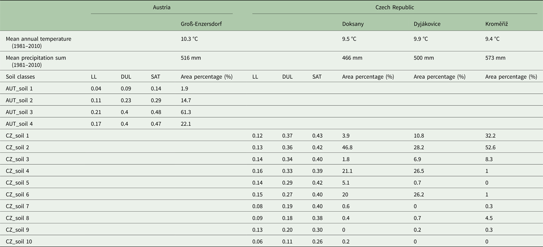
For the purposes of the study, three locations in the Czech Republic (Doksany 50°27′N, 14°10′E, 158 m a.s.l.; Dyjákovice 48°46′N, 16°18′ E, 185 m a.s.l.; Kroměřiž 49°17′N, 17°23′E, 201 m a.s.l.) and one location in Austria (Groß-Enzersdorf 48°12′N, 16°33′E, 157 m a.s.l.) were chosen (Fig. 1). The area comprising these locations is influenced by a continental-type climate, where winters are usually cold, with frequent strong frosts and limited snow cover, and summers are hot and periodically dry (Table 1). The four locations were situated in the middle of the ASCAT pixel (Fig. 2).

Fig. 1. General map of the four study locations Doksany, Kroměřiž, Dyjákovice and Groß-Enzersdorf.
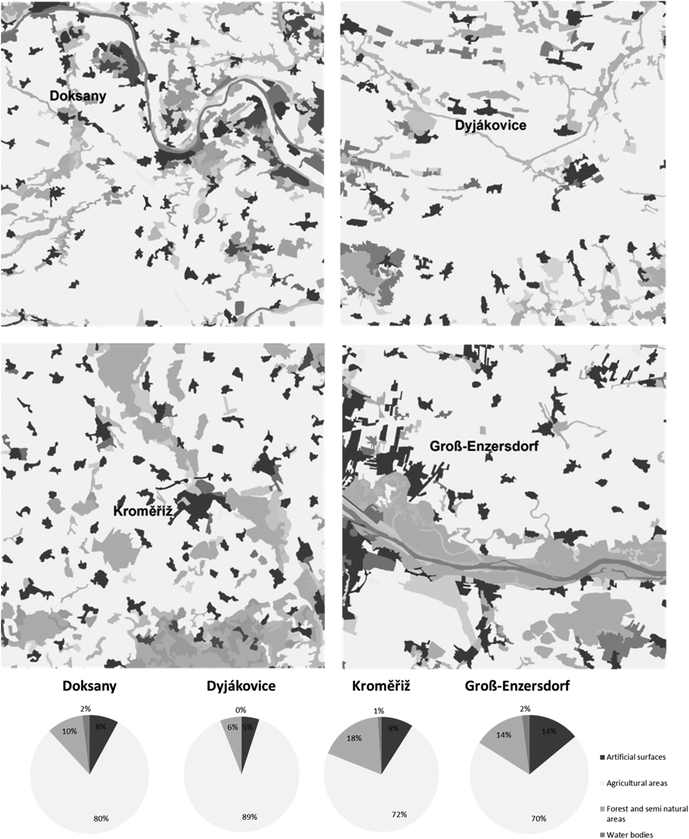
Fig. 2. Corine map 2012 and the land use acreages (in %) according to the Corine Land Cover data 2006 and 2012 of the four investigated grid areas representing years 2007–2011.
Table 1. Mean annual temperature and precipitation sum (1981–2010) of Groß-Enzersdorf, Doksany, Dyjákovice and Kroměřiž as well as the soil water characteristics (up to 1 m soil depth) and area percentage of the different soil classes in Austrian (AUT_soil) and Czech sites (CZ_soil)
LL, lower limit of plant extractable soil water; DUL, drained upper limit; SAT, saturated soil water content.
Corine Land Cover data 2006 and 2012 (http://land.copernicus.eu/pan-european/corine-land-cover) were used for assessing land cover within the ASCAT pixel. These data revealed that land use of the four ASCAT grids were characterized by mainly agricultural land use, to similar extents (0.70–0.90), which was also mostly non-irrigated arable land (Doksany = 0.87; Dyjákovice = 0.89; Kroměřiž = 0.93; Groß-Enzersdorf = 0.93 of arable land). From further statistical reports of the larger region representing Groß-Enzersdorf, around 0.25 were covered by summer crops (such as maize) and 0.75 by winter crops (such as cereals). The highest acreage of artificial surfaces among all four study site grids was visible in Groß-Enzersdorf with around 0.14, including also some Vienna suburbs. Kroměřiž was characterized by a higher acreage of forest and semi-natural areas (0.18). Water bodies occupied only small areas from 0.0 (Dyjákovice) to 0.02 (Doksany and Groß-Enzersdorf) of the grid land cover (Fig. 2).
Soil moisture measurement
All three Czech sites were part of the soil moisture measurement network of climatological stations, which monitor soil moisture content at the 0–0.1 m, 0.1–0.5 m and 0.5–0.9 m layers using sensors placed within the natural soil profile under short grass cover (Možný et al. Reference Možný, Trnka, Zalud, Hlavinka, Nekovar, Potop and Virag2012). The stations use three sensors, one horizontal and two vertical. A detailed pedological survey to determine the wilting point (lower limit of plant extractable soil water = LL) and field capacity (drained upper limit = DUL) was carried out for all layers (Kirkham Reference Kirkham2014). Sensors were first installed at the Doksany station in 1991. Since 1998, the measurement system has also been introduced at other stations. The original measurements using VIRRIB sensors (www.amet.cz) had been gradually replaced by the more accurate TRIFO3G sensors (www.asconsult.cz). Both sensors use the dielectric method to measure soil moisture (Topp et al. Reference Topp, Davis and Annan1980). TRIFO3G sensors featured a high-quality three-rod probe for permanent use in different soils. The standard length of the 100% stainless steel probe is 0.4 m. TRIFO3G sensors have an accuracy of ±1% for volumetric soil moisture measurements under controlled laboratory conditions and are factory-calibrated for most agricultural soils. Measurements can be carried out in both extreme clay soils and sandy soils.
The soil water content measurement for Austrian arable soil was taken from an agrometeorological station of a representative site near Groß-Enzersdorf, where the atmospheric model input parameters were measured. The Campbell Scientific CS615 water content reflectometer (Campbell Scientific Inc. 1995) was used to measure the volumetric water content from 0 to 30 cm soil depth under a natural grass canopy. All measured data used are based on 10-min measurement intervals.
The four stations measured volumetric soil water content at different soil depths under short grass cover. The daily mean soil water content at 0–40 cm in the three Czech Sites and 0–30 cm in Groß-Enzersdorf was used to calculate plant available soil moisture (ASM). Plant ASM data were derived from the history of measurements: long-term reasonable minimum was used as the lower limit (i.e. wilting point) and maximum as the upper limit (i.e. field capacity). The result was given as an ASM percentage (%), where the wilting point of soil represented a value of 0% and field capacity corresponded to 100%. In the case of Kroměřiž station, observed soil water content was missing for the period from March to 9 June 2010 due to technical problems with measurements and for Groß-Enzersdorf these data were only available from 2007 until 2010. The set of stations included within the study was selected after careful consideration. For this reason, the winter periods were omitted from the analysis, because of problems due to soil water often appearing in the form of ice.
Models for simulating soil-crop water balance applied
Two diverse model approaches were applied, differing in the complexity of simulated processes of crop growth and soil-water balance processes.
(i) Decision Support System for Agrotechnology Transfer is a software application program, which comprises crop simulation models for over 40 crops. They are process-based, management-oriented models, which simulate the daily time-step effects for instance of the cultivar, crop management, weather, soil, water and nitrogen on crop growth, phenology and yield (Jones et al. Reference Jones, Keating and Porter2001, Reference Jones, Hoogenboom, Porter, Boote, Batchelor, Hunt, Wilkens, Singh, Gijsman and Ritchie2003). The CERES and CSM-CROPGRO models are part of the DSSAT (v4.0.2.0) software (Jones et al. Reference Jones, Hoogenboom, Porter, Boote, Batchelor, Hunt, Wilkens, Singh, Gijsman and Ritchie2003). In the current study, CERES-Barley (Otter-Nacke et al. Reference Otter-Nacke, Ritchie, Godwin and Singh1991) and CERES-Maize (Jones & Kiniry Reference Jones and Kiniry1986) were examined. The one-dimensional soil water balance model in DSSAT was developed by Ritchie & Otter (Reference Ritchie, Otter and Willis1985; Jones & Ritchie Reference Jones, Ritchie, Hoffman, Howell and Soloman1991; Jones Reference Jones, Penning de Vries, Teng and Metselaar1993; Ritchie Reference Ritchie, Tsuji, Hoogenboom and Thornton1998) and computed the daily change in soil water content by soil layer due to infiltration of rainfall and irrigation, vertical drainage, unsaturated flow, soil evaporation and root water uptake processes. Soil evaporation, plant transpiration and root water uptake processes were separated out in the new DSSAT-CMS into a soil-plant-atmosphere module to create more flexibility for expanding and maintaining the model. Water content varied between LL, DUL and the saturated soil water content (SAT) in each soil layer. Once the water content of a given layer was above DUL, water was drained to the next layer with the ‘tipping bucket’ approach, a profile-wide drainage coefficient. If available, saturated hydraulic conductivity (K sat) for water flow of each specific soil layer could be added to control vertical drainage from one layer to the next. This feature permitted soil to retain water above the DUL for layers that had sufficiently low K sat for water flow. In that case, soil layers may become saturated for sufficient time to cause root death, reduced root water uptake, anoxia-induced stress and decreased nitrogen (N) fixation. Water between SAT and DUL was available for root uptake subject to the anoxia-induced problem, which was triggered when air-filled pore space fell below 2% of total volumetric pore space (Boote et al. Reference Boote, Sau, Hoogenboom, Jones, Reddy, Ahuja, Sassendran and Yu2008). Soil water infiltration was the difference between precipitation and surface runoff, which was calculated using the soil conservation service (SCS) method (Soil Conservation Service 1972). In addition, the model included a modification to the SCS-curve number (SCS-CN) method by Williams et al. (Reference Williams, Jones and Dyke1984), which compensated for soil layers and also for initial soil water content at the time of precipitation. Irrigation was supposed as an additive component of total precipitation (Jones et al. Reference Jones, Hoogenboom, Porter, Boote, Batchelor, Hunt, Wilkens, Singh, Gijsman and Ritchie2003).
The soil-plant-atmosphere module calculated evaporation of water from the soil surface and root water uptake (transpiration) from each layer and communicated this to the soil water balance module. Each day, the soil water content of each layer was updated by adding or subtracting daily water flows to or from the layer as a result of each process (Hoogenboom et al. Reference Hoogenboom, Jones, Porter, Wilkens, Boote, Batchelor, Hunt and Tsuji2003).
(ii) The SoilClim model (Hlavinka et al. Reference Hlavinka, Trnka, Balek, Semerádová, Hayes, Svoboda, Eitzinger, Možný, Fischer, Hunt and Žalud2011) was specifically designed and validated to describe soil moisture and soil temperature. The key water balance components of SoilClim are based on a modification of the concept and model formulation in FAO Irrigation and Drainage paper No. 56 (Allen et al. Reference Allen, Pereira, Raes and Smith1998), including the Penman-Monteith approach for reference evapotranspiration estimates. SoilClim considered dynamically simulated vegetation cover development, from which crop coefficients (K c) for estimates of soil evaporation (in case of bare soil) and crop evapotranspiration (after crop emergence) were derived. In addition, changes in root depth, crop height and leaf area index (LAI) and its effect were also assumed. The soil profile was divided into two layers of 0–40 cm and 40–100 cm depth. Also, in this case, the ‘tipping bucket’ approach was used to estimate soil water content and actual evapotranspiration as a function of water availability. It also considered snow cover effect through the SnowMAUS module (Trnka et al. Reference Trnka, Kocmánková, Balek, Eitzinger, Ruget, Formayer, Hlavinka, Schaumberger, Horáková, Mozný and Zalud2010), proportional runoff in case of precipitation above a certain threshold and partial percolation (simplified imitation of macropore flow), but did not account for a capillary rise from deeper layers. Compared with the crop models, it did not account for the lasting effect of drought on the canopy (in principle, the LAI was not reduced as a result of water stress) and it estimated only LAI value, not the total above-ground biomass. Therefore, the crop component and, in particular, negative feedback between drought intensity and biomass development was greatly simplified (Hlavinka et al. Reference Hlavinka, Trnka, Balek, Semerádová, Hayes, Svoboda, Eitzinger, Možný, Fischer, Hunt and Žalud2011).
Metop Advanced SCATterometer soil moisture
ASCAT is a real-aperture radar onboard the series of Metop satellites. Two Metop satellites are currently operational in the same sun-synchronous orbit (Metop-A since 2006 and Metop-B since 2012), separated by 50 min. The launch of a third and final Metop satellite (Metop-C) is planned in 2018. The ASCAT instrument measures the Normalized Radar Cross Section (NRCS), also called backscatter, at C-band (5.255 GHz) in vertical polarization (VV) (Figa-Saldaña et al. Reference Figa-Saldaña, Wilson, Attema, Gelsthorpe, Drinkwater and Stoffelen2002). The spatial resolution of the ASCAT Level 1b backscatter products is either 25–34 km or 50 km, depending on the filter size used to average the Level 1b full resolution product. The revisit time for central Europe is usually once or twice a day for one Metop satellite. The SSM product was retrieved from the backscatter measurements, using a time series-based change detection approach initially developed for the ERS-1/2 scatterometers by Wagner et al. (Reference Wagner, Lemoine and Rott1999). A new inter-annual vegetation correction has been used in the soil moisture retrieval algorithm, which deviates from the original formulation using climatology in order to account for seasonal vegetation biases. This new feature and other improvements are planned for implementation in the official Metop ASCAT soil moisture products generated and distributed by the Satellite Application Facility on Support to Operational Hydrology and Water Management (H SAF, http://hsaf.meteoam.it) project in the near future. The derived SSM product had a spatial resolution of 25–34 km and corresponded to a depth of 2–3 cm. The soil moisture information was defined by the degree of saturation ranging from 0% (dry, corresponds to a wilting point) to 100% (wet, corresponds to saturated soil water content). In order to obtain soil moisture at deeper soil layers from remotely sensed SSM products, the so-called soil water index (SWI) can be computed. The soils in the study areas were mainly medium soil types according to their soil water storage capacity and did not vary much. The SWI attempted to estimate root-zone soil moisture using an exponential filter approach proposed by Wagner et al. (Reference Wagner, Lemoine and Rott1999) based on a two-layer water balance model. The computation of SWI depended only on a single parameter, the characteristic time T, defined in days. This related to infiltration time and characterized the temporal variation of soil moisture in the root-zone profile. However, T could not be related to a certain depth, since the infiltration rate depended on various soil properties. An appropriate T value needed to be empirically defined depending on the study area and application. In the current study, SWI was computed using T = 2 days (ASCAT SWI T2), which gave a good compromise between high-frequency components from precipitation events and root-zone changes. There could be a certain absolute bias related to the applied soil water capacity; however, relative trend changes should still be well represented, which was the focus of the comparison. The impact of spatial variability of precipitation on soil water balance was normally higher relative to the soil impact during summer in the case study region. An attempt to assess the quality of ASCAT SWI using in situ data from the International Soil Moisture Network had shown good agreement (Paulik et al. Reference Paulik, Dorigo, Wagner and Kidd2014), giving confidence in the root-zone representativeness of SWI. This approach is simple, but no study has yet shown that advanced approaches give superior results that would justify the added complexity of the approach (Manfreda et al. Reference Manfreda, Brocca, Moramarco, Melone and Sheffield2014). In addition, more and more researchers are attempting to relate profile and SSM directly with statistical methods such as neural networks. These methods also work quite well despite being, in practice, as simple as the SWI.
Data processing
The time period considered in the current study for comparison of the different approaches of soil water content determination ranged from 2007 until 2011. For the evaluation, only the months March to September were used. Maize and spring barley crops were simulated in daily steps with the CERES models, while SoilClim simulated grass, maize and spring barley, also daily. The different plants were simulated on the one hand to cover the whole growing season with crops (spring barley and maize) and on the other hand to achieve a plant diversity representative of the region. The growing season for spring barley was from March until July, and for maize was from May until September/October. The DSSAT simulations included only the period of sowing until maturity, whereas SoilClim simulations covered the whole year; both models started their simulations one day before a predefined sowing date (see below).
The model input requirements included weather and soil conditions, plant characteristics and crop management (Hunt et al. Reference Hunt, White and Hoogenboom2001). Weather input data were obtained from the weather stations Doksany (CZ), Dyjákovice (CZ) and Kroměřiž (CZ), provided by the Czech Hydrometeorological Institute, as well as Groß-Enzersdorf (A), available from the Austrian Met Service (ZAMG) (Fig. 1). The data contained daily maximum and minimum temperature, solar radiation, precipitation, wind speed and air humidity for the period 2007–2011.
Ten soil classes according to available water capacity were applied to the Czech sites Doksany, Dyjákovice and Kroměřiž and four at the Austrian site Groß-Enzersdorf in Marchfeld (Table 1) (Thaler et al. Reference Thaler, Eitzinger, Trnka and Dubrovsky2012, Reference Thaler, Gobin and Eitzinger2017). The relative ASM for the first soil layer of 0–40 cm depth was used to calculate an area-weighted average of the region, forming the basis for soil moisture comparisons. ASM was derived from the soil classes and finally, the model results for each soil profile were recalculated/averaged based on spatial representation.
To validate the two CERES models, simulated outcomes were compared with measured results obtained from field trials. The CERES barley model for spring barley was calibrated for the cultivar ‘Magda’ using agrotechnological, phenological, yield and weather data from an experimental site at Fuchsenbigl, Marchfeld (48°12′N, 16°44′E, 157 m a.s.l.) for the periods 1989–95, 1998 and 2001/02. The discrepancy between simulated and observed dates of anthesis and physiological maturity varied from 0 to 7 days, and the simulated yield was within 20% of the measured values for each year (R 2 = 0.57, RMSE = 623 kg/ha) (Eitzinger et al. Reference Eitzinger, Trnka, Semerádová, Thaler, Svobodová, Hlavinka, Siska, Takác, Malatinská, Nováková, Dubrovsky and Zalud2013b). The CERES-maize model was calibrated in the same way and verified for the periods 1998–1999 and 2001–2002 using data for the cultivar ‘Parzival’. The difference between simulated and observed dates of maize anthesis for calibration varied from 0 to 4 days. Simulated grain yields mostly agreed with the measured data (R 2 = 0.93, RMSE = 153 kg/ha) and the deviation in annual yield predictions was <20%.
SoilClim was not calibrated using any specific cultivars because the real representation of cultivars within individual regions was unknown. Spring barley, maize and grass parameters were based on calibrations described in Hlavinka et al. (Reference Hlavinka, Trnka, Balek, Semerádová, Hayes, Svoboda, Eitzinger, Možný, Fischer, Hunt and Žalud2011). For grass, the cover was approximated not directly to certain species but for typical regularly cut cover from meteorological stations. This calibration was based on Allen et al. (Reference Allen, Pereira, Raes and Smith1998) and soil moisture measurements from four stations in Central Europe and 14 stations in the USA (Hlavinka et al. Reference Hlavinka, Trnka, Balek, Semerádová, Hayes, Svoboda, Eitzinger, Možný, Fischer, Hunt and Žalud2011).
All simulations were conducted for rain-fed farming conditions for spring barley, maize and grass, respectively. The sowing date was calculated with predefined temperature sums from 1 January: a temperature sum of 80 °C was used as sowing date for spring barley and 520 °C for maize (temperature base 0 °C). This approach was selected since there were no experiments that would appropriately represent the conditions through the all selected regions and included years. Further initial conditions of soil water content according to measured values on grassland sites one day before sowing were added in both models. For spring barley, grass can be used as a good reference, because grass is not actively growing earlier at the case study site after the winter period when barley is sown, and thus the water balance after the dormant winter period should be very similar. Maize is sown about 4–6 weeks later where grass is already growing, having additional water use as compared with bare soil. The difference in evaporation of short grass compared with bare soil is, however, relatively small (K c factor about 0.2 v. 0.4) and the uncertainty from, e.g. spatial precipitation variability in comparison with the other scales applied can be much higher. The relatively small error coming from this assumption is therefore limited. Spring barley was fertilized with 40 kg N/ha, 25 kg phosphorus (P)/ha and 170 kg potassium (K)/ha at tillering (growth stage (GS) 21–23, Zadoks et al. Reference Zadoks, Chang and Konzak1974) and 40 kg N/ha at stem elongation or jointing (GS 31–33), the amount that farmers currently use in these areas. Maize simulated fertilization of 80 kg N/ha, 39 kg P/ha, 166 K/ha at tillering (GS 21–23) and 55 kg N/ha at stem elongation or jointing (GS 31–33).
Methods used for evaluating and comparing model performance
The DSSAT crop growth models, soil water balance model (SoilClim) and remote sensing based (Metop ASCAT) estimated soil moisture were evaluated with measured soil moisture values. Here, ASM, calculated from the model outputs and measured values, and the degree of saturation (%) from ASCAT SWI T2 were compared. The comparison of soil moisture measured by remote sensing satellites and in situ instruments was complicated by the fact that different spatial and temporal variabilities (e.g. land use, soil composition, mean soil water content, etc.) influenced the soil moisture characteristics (Nicolai-Shaw et al. Reference Nicolai-Shaw, Hirschi, Mittelbach and Seneviratne2015). In order to verify the spatial and temporal representativeness, soil moisture from two global land surface models was used as an additional data source. The ERA-Interim/Land data set from the European Centre for Medium-Range Weather Forecasts represented a global atmospheric reanalysis including 6-hourly land surface parameters for the period 1979–2010 (Balsamo et al. Reference Balsamo, Albergel, Beljaars, Boussetta, Brun, Cloke, Dee, Dutra, Pappenberger, De Rosnay, Sabater, Stockdale and Vitart2012). The spatial resolution of the data set was approximately 80 km and soil moisture information was provided for four depth layers (0.00–0.07 m, 0.07–0.28 m, 0.28–1.00 m and 1.00–2.55 m). The second data set was based on the Noah model provided by NASA's Global Land Data Assimilation System (GLDAS) and contained atmospheric and land surface parameters on a global 0.25° grid (Rodell et al. Reference Rodell, Houser, Jambor, Gottschalck, Mitchell, Meng, Arsenault, Cosgrove, Radakovich, Bosilovich, Entin, Walker, Lohmann and Toll2004). From early 2000-ongoing, the GLDAS Noah data set provided 3-hourly soil moisture observations for four layers (0.00–0.10 m, 0.10–0.40 m, 0.40–1.00 m and 1.00–2.00 m). For both land surface models, soil moisture from the second layer was used as a qualitative reference in order to understand soil moisture dynamics at a spatial scale comparable with Metop ASCAT. Global Land Data Assimilation System and ERA-Interim/Land were used only for the visual presentation and not for calculations.
In the current study it was hypothesized that, (i) at site level, ground-based modelling should provide estimates of soil moisture with higher accuracy compared with the Metop ASCAT soil moisture product and (ii) the process-based crop model (DSSAT) should provide superior results compared with the simple water balance model (SoilClim), particularly under frequent water stress conditions. In addition, it was expected that (iii) the Metop ASCAT soil moisture product would provide a good estimate of annual changes in water availability and that (iv) it would be able to distinguish extreme (drought/wet) seasons, making it a potential tool for regional drought monitoring.
For assessing and comparing model performance, a set of statistical parameters was calculated: the root mean square error (RMSE), the mean absolute error (MAE), the percent bias (PBias), the index of agreement (d) and the least-squares coefficient of determination R 2. The measured values were used as ‘ground truth’ references for the relative changes, not for absolute soil water content. The relative change (decreasing or increasing of soil water content trend at any time) should be reflected regardless of vegetation cover, in particular for short-term changes chiefly driven by precipitation and soil evaporation. Differences in evaporation from vegetation may, however, introduce slight biases depending on the season and crop-specific water needs.
Beside the classical model performance metrics, Triple Collocation Analysis (TCA) was also applied. This is a statistical tool used for error characterization, first introduced by Stoffelen (Reference Stoffelen1998) and defined as follows:
 $$i = \; \alpha _i + \; \beta _i{\rm \Theta} + \; \varepsilon _i\quad \; i\,{\rm elem}\,[X,\,Y,\,Z]$$
where [X, Y, Z] presents three spatially and temporally collocated data sets; Θ is the unknown true soil moisture state; α i and β i are systematic additive and multiplicative biases of data set i in terms of the true state, and εi is additive zero-mean random noise. The following assumptions are made by the error model: (i) true soil moisture signal and the observations are linear, (ii) signal and error stationarity, (iii) errors and the soil moisture signal are independent (error orthogonality), and (iv) errors of the three spatially and temporally collocated data sets are independent (zero error cross-correlation) (Gruber et al. Reference Gruber, Su, Zwieback, Crow, Dorigo and Wagner2016). More detail about the computation and consequences if certain assumptions are not met can be found in Gruber et al. (Reference Gruber, Su, Zwieback, Crow, Dorigo and Wagner2016). Triple Collocation Analysis simultaneously estimates the error variances of three spatially and temporally collocated data sets, which are related linearly to the hypothetical (unknown) truth with uncorrelated errors, introduced a new representation of the error in terms of Signal-to-Noise ratio (SNR):
 $$SRN_i[dB] = 10\log (SNR) = 10\log \displaystyle{{\beta _i^2 \sigma _{\rm \Theta} ^2} \over {\sigma _{\varepsilon _i}^2}} $$
 The SNR, expressed in dB, indicates the relationship between signal variance and noise variance;  $\sigma _i^2 $ presents the data set variances. For example, 0 dB means that the signal variance is equal to the noise variance, and ±3 dB means that the signal variance is twice/half that of the noise variance. Triple Collocation Analysis does not assume any of the data sets to represent the ‘ground truth’ (Gruber et al. Reference Gruber, Su, Zwieback, Crow, Dorigo and Wagner2016).
Results
Overall assessment of model performances for the four study sites
Five years (2007–2011) of daily in situ soil moisture measurements for all four weather station sites together were compared with model data and the Metop ASCAT soil moisture product. The linear regression model was able to explain between 23% (ASCAT SWI T2) and 58% (CERES-Barley) of the variance by the model (R 2); thus, from poor correspondence to rather good. The relative average difference between model estimates and in situ measurements (RMSE) for ASM was 19–21% in all crop models and 26% in the ASCAT SWI T2. The lowest variation and RMSE could be found in CERES-Barley, the highest in ASCAT SWI T2 (results not shown).
The comparison between measured and different simulated or estimated soil moisture for all four study areas separately is presented in Fig. 3. The data sources include point-scale from in situ data, plot-scale from model simulation and large-scale from satellite data. In Doksany, SoilClim and ASCAT SWI T2 show good agreement with measured values. In the time-frame 2007 and 2009, ASCAT SWI T2 captured soil moisture in Djakovice very well. In Kroměřiž, ASCAT SWI T2 underestimated ASM during the two humid vegetation periods 2010 and 2011, whereas the models fit well with in situ values. The models and Metop ASCAT in Groß-Enzersdorf agree very well between 2007 and 2009. Comparing the time series to ERA-Interim/Land and Noah GLDAS indicates that both global land surface models show only large-scale variations and are not able to capture the fine daily changes of a single in situ station. Normally, data are matched in order to remove systematic differences related to scale, layer depth and measurement/model characteristics (Brocca et al. Reference Brocca, Melone, Moramarco, Wagner, Albergel and Petropoulos2013).

Fig. 3. The course of in situ measured, models simulated (DSSAT and SoilClim), remote sensing (ASCAT SM, ASCAT SWI T2) and modelled (ERA and Noah GLDAS) estimations of soil water content during 2007–2011 in Doksany, Dyjákovice, Kroměřiž and Groß-Enzersdorf. Model estimates and in situ measurements represent a soil depth of 0–40 cm.
A 30-day moving average, showing the differences between soil moisture measured, simulated and estimated, is presented in Fig. 4. This approach should help to remove seasonal influences and uncover similar short-term anomalies. The daily soil moisture values were compared with the moving average and it was determined whether they exceeded or fell below the mean values. Seasonal biases can be seen in all data sources due to scale differences, different layer depth and seasonal biases based on shortcomings of the measurements and models.

Fig. 4. 30-day moving average of soil moisture and their daily deviations for CERES-Maize, SoilClim-Maize, ERA-Interim/Land, ASCAT SWI T2 and in situ for Doksany, Dyjákovice, Kroměřiž and Groß-Enzersdorf (grey = below and black = exceeded the moving average). Model estimates and in situ measurements represent a soil depth of 0–40 cm.
Often, SoilClim-Maize simulated ASM better than CERES-Maize; furthermore, in all the stations apart from Doksany, ASCAT SWI T2 showed good agreement, especially in 2009 and 2010.
The site-specific model and ASCAT SWI T2 performances are included in Table 2 based on measured soil water content. During the 5 years investigated (March–September periods), the analogies between Doksany and Kroměřiž were very striking. In fact, in both cases, the crop model DSSAT and ASCAT SWI T2 underestimated soil moisture in the first soil layer, whereas SoilClim generated overestimates. Moreover, for these sites the lowest MAE (10–16% ASM), RMSE (14–21% ASM) and highest d (0.8–0.9) results could be found in CERES-Barley and CERES-Maize. On the other hand, the PBias for ASCAT SWI T2 showed the best average tendency of the simulated values (−7%) in Doksany.
Table 2. Comparative statistics (MAE, RMSE, PBias, d and R 2) of model performance against measured soil water contents for the four study areas from March until September

In Groß-Enzersdorf, as in the previous two stations, CERES-Barley performed best (for all the main parameters) followed by SoilClim-Grass. Special mention must be made of the very low PBias of just 2.9% in CERES-Maize.
Dyjákovice, on the other hand, behaved differently: the SoilClim simulations (barley and maize) presented the lowest MAE (14% ASM), RMSE (19% ASM) and PBias (−10 to −12%) values and all simulations tended to underestimate the first soil moisture layer. The index of agreement with a value of 0.7–0.8 indicated good simulation quality and the R 2 ranged from 0.4 to 0.6.
In a second step, TCA was applied for the four study areas. Figure 5 presents the SNR and R 2 for measured (in situ), ASCAT as well as the different models (third reference). Of particular note was the low R 2 value of ASCAT in the CERES-Maize simulations (with the only exception of Groß-Enzersdorf). This was reflected also by the negative SNR for ASCAT, whereas the measured values showed a high signal. In other words, measured and simulated values presented similar signals, whereas ASCAT did not fit in.

Fig. 5. Triple Collocation analysis and r 2 for Doksany, Dyjákovice, Kroměřiž and Groß-Enzersdorf. Measured = point scale, third reference = local scale (different models) and large scale = ASCAT.
It must be noted that the sample size could have an effect on SNR since its uncertainty increased with decreasing number of samples (Zwieback et al. Reference Zwieback, Scipal, Dorigo and Wagner2012). This effect could be seen for measured and ASCAT SNR, which should indicate a similar behaviour to the third reference. However, the SNR values were spread. In addition, the requirements of the error model (see above) might not all be perfectly fulfilled, which was another source of uncertainty in the SNR results.
The highest variation could be found in Kroměřiž, whereas in Dyjákovice all the three approaches present similar results with an R 2 between 0.4 and 0.6 and SNR around 3 dB, meaning that the signal variance was twice as high as the noise variance (except for CERES-Barley). Dyjákovice was also the study site, which demonstrated a different behaviour for the classic statistical parameters to the other three locations (see above and Fig. 6).

Fig. 6. Mean monthly measured values and RMSE for the four study sites Doksany, Kroměřiž, Dyjákovice and Groß-Enzersdorf.
The performance of the model's soil water balance outputs may change during the growing season due to deviations of simulated v. real vegetation dynamics, which can influence models’ site-specific, as well as ASCAT SWI T2, uncertainties. In the latter, this is an issue of deviations of spatial crop type acreages as it represented grid averaged values. In the following, the differences of simulated and measured soil moisture, RMSE, PBias and d for each study area for monthly as well as growing season time scales are discussed (Tables 3–6).
Table 3. Doksany: differences of simulated and observed soil moisture, RMSE (% ASM), PBias (%) and Index of Agreement for month and growing season (gs) 2007–2011

Table 4. Dyjákovice: differences of simulated and observed soil moisture, RMSE (% ASM), PBias (%) and Index of Agreement for month and growing season (gs) 2007–2011

Table 5. Kroměřiž: differences of simulated and observed soil moisture, RMSE (% ASM), PBias (%) and Index of Agreement for month and growing season (gs) 2007–2011

Table 6. Groß-Enzersdorf: differences of simulated and observed soil moisture, RMSE (% ASM), PBias (%) and Index of Agreement for month and growing season (gs) 2007–2010

Performance of available soil moisture estimates at different periods of the growing season
Combining data from all four stations into one data set revealed low deviation of monthly means between measured and simulated ASMs at the beginning of the growing season for CERES-Barley (March), CERES-Maize (April) and SoilClim-Maize (April). In particular, the models at Doksany and Kroměřiže performed better than the other sites and their RMSE values were low. SoilClim-Barley and SoilClim-Grass did not show this behaviour to that extent. It should be borne in mind that the measurement sites were under short grass with relatively small changes in root water uptake due to very low seasonal change in active above-ground biomass, in comparison with the simulated crops with a higher seasonal variation of biomass-driven water demand. Thus, the better agreement in the early season with low crop biomass can be explained.
The monthly difference between measured ASM and ASCAT SWI T2-based SM was relatively high compared with ASM based on the crop model outputs. From March until May these differences were mainly negative, and the PBias also presented an underestimation (except at Groß-Enzersdorf), but from July the ASCAT SWI T2 estimations were principally overestimated.
At all locations, the CERES models, apart from CERES-Maize in Kroměřiže, showed primarily a negative PBias during periods of the fully established canopy (barley: May–July and maize: June–September) caused by seasonal above-ground biomass change. In contrast, the SoilClim soil water content outputs here more often showed a positive PBias, with the only exception of Dyjákovice, being the most humid place.
The results from this comparison showed that simulated soil moisture values vary widely at all sites and in all years due to the dynamics in above-ground biomass, besides the weather conditions. However, an almost tripartite behaviour could be found when the incidence of wet periods on soil moisture simulation performances were observed. In fact, DSSAT performed best for dry periods and although ASCAT simulated well for moderate soil moisture, soil water contents and related ASM during wet periods were well simulated by SoilClim (with only a few exceptions) (Tables 3–6).
Performance of available soil moisture estimates under dry, moderate and wet soil conditions
Considering all four sites, soil water contents and related ASM of dry periods were best simulated by DSSAT models while CERES-Maize performed very well under moderate dry and CERES-Barley under extremely dry conditions. Overall, DSSAT models simulated realistically up to 30% ASM. There are only a few outliers observed in Groß-Enzersdorf (April 2009) and Kroměřiže (June–July 2009) for unknown reasons. The RMSE values were also quite low in this range, especially in Doksany, being the driest place in the current study (Fig. 6).
Mainly positive differences between simulated and measured soil moisture could be seen during dry periods in all the four locations for the SoilClim simulations (up to 50% ASM). High RMSE values were also seen here, especially in Kroměřiže (Fig. 6). The PBias showed high positive values during very dry periods, especially in Doksany, Groß-Enzersdorf and Kroměřiže, whereas in humid periods the model generally underestimated (Tables 3–6).
Another very interesting pattern could be seen at Doksany, Dyjákovice and Kroměřiž, where the average monthly RMSE (respectively, 20 and 26% ASM) of the ASCAT SWI T2 estimations were considerably higher but at the same time the RMSE standard deviation of ASCAT SWI T2 (6 and 10% ASM) was much lower than in the different crop models. An exceptional case was given in Groß-Enzersdorf, where almost all the crop models (with the only exception of CERES-Maize) obtained a very low RMSE standard deviation (results not shown).
Advanced SCATterometer SWI T2 grid-based estimates performed at its best for moderate soil moisture conditions at all sites between 30 and 50% of the site-based measured ASM. In this range, the product showed also the lowest RMSE values in all cases (Fig. 6). Below about 30% ASM, ASCAT SWI T2 showed a positive difference between observed and simulated ASM, but a negative difference above this limit. The same pattern was shown by PBias, with a threshold of 33% ASM. By looking at the whole growing season, ASCAT SWI T2 estimations corresponded best to reality when the measured soil moisture ranged between approximately 30% and 50% ASM (Doksany 38–47; Dyjákovice 31–52; Kroměřiže 34–36 and Groß-Enzersdorf 29–37%) (Tables 3–6).
An extreme drawback of using ASCAT was noticed during very humid periods, where the RMSE scored very high (Fig. 6). Advanced SCATterometer was not able to catch high daily precipitation sums. In general, all crop models also showed a negative difference during very humid seasons, but less than ASCAT-based ASM estimates (results not shown).
SoilClim-Maize and Barley showed the best performance in Doksany, Kroměřiže and Groß-Enzersdorf during wet soil conditions. However, for Dyjákovice only SoilClim-Grass was a good predictor for humid periods, whereas during dry periods SoliClim-Maize and Barley showed the lowest differences (until 60% ASM) and shared a similar behaviour with DSSAT (Tables 3–6).
In Doksany and Groß-Enzersdorf, RMSE v. mean monthly measured values showed a large spread, whereas Dyjákovice and Kroměřiže showed clearer trends (Fig. 6). In Dyjákovice, the RMSE increased with humidity in all approaches. In Kroměřiže, during dry periods, high SoilClim RMSE values for coupled to very high ASCAT RMSE during wet months could be found.
Model ranking
In the next step, potential seasonal changes of model performance in the estimation of ASM was investigated. For each month during the period 2007–2011 the first three best models, which fit to the measured soil moisture, were identified. The result was based on the difference of measured and simulated values and filtered out (Table 7).
Table 7. The first three best ranking models according to their performance on estimated monthly mean ASM against ASM based on measured soil moisture (2007–2011). Maize simulations only start with month May, whereas CERES-Barley simulations ending in June, and were therefore not considered in the remaining months

As already indicated previously, the CERES simulations in arable regions performed better in the first 5 months, under conditions of canopy establishment (March–April: CERES-Barley and May–June: CERES-Maize). SoilClim performed at its best in August and September. It seemed that this model performs better under grass and bare soil conditions, which could be caused by the better representation of the real canopy cover and related seasonal root water uptake of measurement sites. ASCAT SWI T2 came in second and third place, respectively, in the three summer months.
Discussion
Due to climate change, water scarcity, drought frequency and severity are increasing globally, especially affecting agriculture and food production. Even locally, changes in the modelled and observed soil water content have been reported, especially in May and June (Trnka et al. Reference Trnka, Brázdil, Možný, Štěpánek, Dobrovolný, Zahradníček, Balek, Semerádová, Dubrovský, Hlavinka, Eitzinger, Wardlow, Svoboda, Hayes and Žalud2015a) and explained by a significant increase of temperatures and global radiation and decrease in precipitation (Trnka et al. Reference Trnka, Brázdil, Balek, Semeradova, Hlavinka, Možný, Štěpánek, Dobrovolný, Zahradníček, Dubrovsky, Eitzinger, Fuchs, Svoboda, Hayes and Žalud2015b), together with significant shifts in weather circulation patterns (Trnka et al. Reference Trnka, Kysely, Možny and Dubrovsky2009). These changes have been recently attributed to increased carbon dioxide (CO2) concentrations (Brázdil et al. Reference Brázdil, Trnka, Mikšovský, Řezníčková and Dobrovolný2015); moreover, the frequency of drought in recent decades is among the highest ever recorded in the past 500 years (Brázdil et al. Reference Brázdil, Dobrovolný, Trnka, Kotyza, Řezníčková, Valášek, Zahradníček and Štěpánek2013). Therefore, decision-makers in the agriculture and hydrology sectors need to improve water use efficiency, especially in crop production, which was shown to be particularly affected (Hlavinka et al. Reference Hlavinka, Trnka, Semerádová, Dubrovsky, Zalud and Možný2009; Thaler et al. Reference Thaler, Eitzinger, Trnka and Dubrovsky2012; Eitzinger et al. Reference Eitzinger, Trnka, Semerádová, Thaler, Svobodová, Hlavinka, Siska, Takác, Malatinská, Nováková, Dubrovsky and Zalud2013b). At the same time, soil moisture availability has been shown to be important for grassland production (Trnka et al. Reference Trnka, Eitzinger, Gruszczynsk, Buchgraber, Resch and Schaumberger2006) and also for various tree species including fir (Büntgen et al. Reference Büntgen, Bràzdil, Dobrovolný, Trnka and Kyncl2011), oak (Rybníček et al. Reference Rybníček, Čermák, Žid, Kolář, Trnka and Büntgen2015) and beech (Kolář et al. Reference Kolář, Giagli, Trnka, Bednářová, Vavrčík and Rybníček2016). The status and development of soil wetness are therefore crucial, becoming a key aspect for well-informed decision making, and relevant tools and methods should deliver representative and reliable spatial information to farmers at the field scale. Remote sensing products such as ASCAT can provide valuable data on spatial soil wetness conditions. Nevertheless, their intrinsic weaknesses lie in representing only surface layers, as well as not always having the fine spatial resolution needed. By combining tools such as site-based crop water balance models with remote sensing methods, a potential for better-performing spatial estimates can be obtained. In the current study, two different crop model (incl. soil-crop water balance) approaches and ASCAT SWI T2 estimates were compared with measured soil water content at four sites under short grass, representing Central European soil and climatic conditions. The comparison included different time scales from daily to yearly for three different main crops and several soil types, and offers insight into seasonal influences of model performance related to crop and weather conditions. The study period was 2007–2011 and included the main growing season months March until September. Here the uppermost soil layer (0–40 cm) was analysed.
The initial hypothesis stated that models driven by local precipitation measurements and site-representative soil characteristics would provide estimates of soil moisture with higher accuracy on the site level in comparison with ASCAT SWI T2. In addition, it was expected that the process-based crop models of DSSAT would provide better results compared with the simple water balance model SoilClim, due to better-simulated dynamics of soil layer specific root water uptake. In case of daily simulations for all the four stations together, the model CERES-Barley presented the lowest variation and overall tended to underestimate soil moisture (average BPias = −14.2%). A negative bias was also reported by Eitzinger et al. (Reference Eitzinger, Trnka, Hösch, Zalud and Dubrovsky2004) in their study based on lysimeter data on similar soil, due to deviations in root water uptake in the deeper soil layers. Advanced SCATterometer SWI T2 daily estimations are, as expected due to spatial averaging, the weakest and their variation is high. The standard deviation of the model prediction error is around 20% ASM for SoilClim-Barley and SoilClim-Grass and not essentially higher as in DSSAT (19% ASM). On the other hand, SoilClim generally overestimates soil moisture.
Although comparisons of in situ soil water measurements can be affected by the high spatial variability of soil water balance determining factors on the small scale, seasonal changes can be represented well. Moreover, the measurement sites are characterized by homogenous permanent grass canopies (and root distribution) reducing spatial inhomogeneity of soil water content.
Regarding the specific model performances during dry periods, it can be observed at all four study sites that DSSAT better simulates the first soil moisture layer (up to 50% ASM measured soil moisture), whereas SoilClim simulations fit quite well during humid months. Therefore, as it was assumed that the process-based crop model DSSAT provides more realistic results in comparison with the simple water balance model SoilClim under frequent water stress conditions, which can be explained by specific processes simulated in more detail and dynamics such as the root and crop growth. On the other hand, DSSAT reacts sensitively to humidity and shows the highest deviations during moist periods. A possible explanation could be that the interception losses are not captured well in the model.
Advanced SCATterometer SWI T2 shows poor results on daily statistical parameters. However, if a longer period, such as a month or a growing season, is taken into account, ASCAT SWI T2 results are more reliable and can deliver a good soil moisture estimate. The model predicts values reasonably well, particularly during conditions of low surface biomass (early vegetation season) of the areas under evaluation. This can be related to the fact that the scatterometer returned better estimates of the water content in the soil layer when the lack of vegetation allowed the signal more ground penetration.
Hence, ASCAT provides good estimates of annual changes in water availability and was able to distinguish extreme (drought/wet) seasons. The performances of Metop ASCAT soil moisture was positively validated and could represent a complementary source for the estimation of crop-soil water balance in Central Europe, e.g. in regional drought monitoring. Furthermore, the in-situ values should be critically judged, because their data quality can be influenced by different measurement errors, for example sensor changes, replacement or calibration, power failure. Due to such limitations of in situ measurements, ASCAT SWI T2 shows more reliability in long-term observations since it is more stable and better at tracking changes from year to year. For in situ measurements, the potential spatial variability at a small scale has to be considered for comparisons at differing scales.
During early and late crop stages, the crop models and ASCAT SWI T2 estimations present a low deviation compared to the measured grass-soil water content. It is an effect of reduced water take up by crops/plants from deeper soil layers during these periods and less expressed vertical soil water differences.
Knowing the time-dependent changing performances of the different methods, depending on changing soil wetness and crop conditions, ranges of varying uncertainty regarding model application and recommended model choices could be given. Advanced SCATterometer SWI T2 performance at its best under medium soil wetness conditions and related to the low variation of precipitation frequency and the amount is obvious. Soil crop water balance models require, in case of more extremes towards drought and wetness, reliable predictions. A significant improvement of spatial estimates of ASM could, therefore, be reached by considering annual actual acreage of crop types, even without high spatial (field-based) crop simulation efforts, especially in regions with similar agroecological (soil, climate, land use) conditions.
Acknowledgements
MT and PH work was supported through the Ministry of Education, Youth and Sports of the Czech Republic project under the National Sustainability Program I (NPU I) – grant number LO1415 and by the Grant Agency of the Czech Republic projects no. 16–16549S as well as 17-10026S which allowed for additional comparison work and obtaining new soil moisture data. JE and ST were supported by the project ‘COMBIRISK’ of the Austrian Climate Research Programme (ACRP) and from the European Union's Horizon 2020 research and innovation programme under grant agreement no. 691998 (Serbia For Excell). The authors would like to thank their national meteorological and hydrometeorological institutes for providing weather data and EUMETSAT's ‘Satellite Application Facility on Support to Operational Hydrology and Water Management (H SAF)’ project for providing Metop ASCAT soil moisture products. GIS support is acknowledged from Dr Daniela Semerádová.


