


Introduction
Nowadays, coverage of genetically modified crops is increasing rapidly which induces contamination risk in conventional or organic crops. Furthermore, there is great variability in cross-pollination rates due to many involved factors which describe pollen and canopy characteristics as well as to their interactions with its environment. It is therefore difficult to understand and account for the risks of cross-pollination only by experimental approaches (Treu and Emberlin, Reference Treu and Emberlin2000). For these reasons and in order to minimize and monitor the risk of this potential and complex problem, various numerical methods have been developed and discussed in the literature (e.g., Dietiker et al., Reference Dietiker, Stamp and Eugster2011; Marceau et al., Reference Marceau, Loubet, Andrieu, Durand, Foueillassar and Huber2011; Torimaru et al., Reference Torimaru, Wennstrom, Lindgren and Wang2012). Maize pollen grains are roughly spherical with diameters around 90 μm and therefore have a high settling velocity compared with other pollen types (Raynor et al., Reference Raynor, Eugene and Janet1972; Di-Giovany et al., Reference Di-Giovanni, Kevan and Nasr1995). As a consequence, dispersed maize pollen quantities are small: 95% of the emitted pollen is deposited within 10 m of the source and 99% at 30 m (Jarosz et al., Reference Jarosz, Loubet, Durand, McCartney, Foueillassar and Huber2003). In order to simulate the dispersal of maize pollen as well as to estimate quantities of released pollen, many physically-based models have been developed:
The Lagrangian stochastic approach was introduced by Jarosz et al. (Reference Jarosz, Loubet and Huber2004), Dupont et al. (Reference Dupont, Brunet and Jarosz2006) proposed an Eulerian approach, while Klein et al. (Reference Klein, Lavigne, Foueillassar, Gouyon and Laredo2003) adopted a statistical approach. Furthermore, several atmospheric dispersion models have been developed recently (see, e.g., Dietiker et al., Reference Dietiker, Stamp and Eugster2011; Zhang et al., Reference Zhang, Duhl, Salam, House, Flagan, Avol, Gilliland, Guenther, Chung, Lamb and VanReken2014; Baklanov et al., Reference Baklanov, Smith Korsholm, Nuterman, Mahura, Nielsen, Sass, Rasmussen, Zakey, Kaas, Kurganskiy, Sørensen and González-Aparicio2017; Zink et al., Reference Zink, Kaufmann, Petitpierre, Broennimann, Guisan, Gentilini and Rotach2017). However, the numerical dispersion models need to be combined with a flow model, whether empirical, Lagrangian or Eulerian, describing the wind profiles and turbulence. In this setting, Arritt et al. (Reference Arritt, Clark, Goggi, Sanchez, Westgate and Riese2007) have developed a three-dimensional Lagrangian model to simulate the dispersion of pollen and have validated the approach on daily measurements of deposition on the ground. Dupont et al. (Reference Dupont, Brunet and Jarosz2006) have compared Lagrangian and Eulerian models with experimental two-dimensional dispersion measurements in the wind direction. The Eulerian model is based on a flow model, Aquilon, in which an advection-diffusion conservation equation is integrated, while the Lagrangian stochastic model, SMOP (Stochastic Mechanistic mOdel for Pollen dispersion and deposition), uses an empirical model of flow. Astini et al. (Reference Astini, Fonseca, Clark, Lizaso, Grass, Westgate and Arritt2009) predict effective rates of cross-pollination at the end of the pollination season using the Lagrangian model of Arritt et al. (Reference Arritt, Clark, Goggi, Sanchez, Westgate and Riese2007) combined with the pollination model of Lizaso et al. (Reference Lizaso, Westgate, Batchelor and Fonseca2003). However, the model input variables are subject to many sources of uncertainties including errors of measurement, absence of information and weak or partial understanding of the driving forces and mechanisms. These impose limits on our confidence in the response (i.e., outputs) of the model. Following an Eulerian model, Dupont et al. (Reference Dupont, Brunet and Jarosz2006) developed an empirical sensitivity analysis for some variables: settling velocity of pollen, Schmidt number, turbulence parameters and percentage of pollen re-entrained in the air after deposition on leaves. Contrary to our setting this methodology does not take into account possible interaction between variables. Good modelling practice requires that the specialists provide an evaluation of the confidence in their models by applying a Sensitivity Analysis (SA). Such an approach is used to study how a variation in the output of a model can be apportioned, quantitatively or qualitatively, in different sources of input variation. For performing a SA of a model, three approach classes are available: Screening Designs (SD), Local Sensitivity Analysis (LSA) and Global Sensitivity Analysis (GSA) described by Saltelli et al. (Reference Saltelli, Chan and Scott2000a). The Monte Carlo method, a GSA, has been applied herein because of its robustness and performance as stated by Saltelli et al. (Reference Saltelli, Chan and Scott2000a, Reference Saltelli, Tarantola and Compolongo2000b). However, its application involves multiple simulations that make it expensive in terms of time taken to perform the analysis. In order to reduce the computation time, the Latin hypercube sampling technique has been used to create a matrix of values used as inputs to the SMOP model. Such a design is able to sample parameter values with a good homogeneous distribution in the parameters' domain as proved by McKay et al. (Reference McKay, Beckmann and Conover1979) and Iman (Reference Iman1992).
Emission of maize pollen could be estimated using plastic bags placed on the tassels (Hall et al., Reference Hall, Vilella, Trapani and Chimenti1982; Jarosz et al., Reference Jarosz, Loubet, Durand, McCartney, Foueillassar and Huber2003). As a shortcoming of this method, tassels in closed environment conditions will induce a greenhouse effect, and as a consequence, this method provides a measure of potential emitted pollen rather than the actual emitted pollen. Due to this fact, Raupach (Reference Raupach1989) and later Jarosz et al. (Reference Jarosz, Loubet, Durand, Foueillassar and Huber2005), Aylor et al. (Reference Aylor, Boehm and Shields2006) and Dupont et al. (Reference Dupont, Brunet and Jarosz2006) provided an alternative approach, which we use in this work, leading to a real emission rate that could be inferred from both measurements and simulations of pollen dispersion.
The objective of the current paper is to present a methodology to infer pollen emission rate taking into account the uncertainty of input variables of the SMOP model on deposition in a small canopy gap. Uncertainty of variables is related to retention of pollen by the plant canopy as well as to pollen aerodynamic characteristics.
Material and methods
Model description
The Lagrangian stochastic SMOP model has been under development in the National Institute of Agronomic Research, France since 2003 (Jarosz et al., Reference Jarosz, Loubet and Huber2004). The model is designed to predict pollen dispersion and deposition downwind and within a flowering field. Displacement of individual pollen grains is given by the following two-dimensional stochastic differential equations.


where t is time; u and w are the horizontal and vertical air particle velocity components, respectively; dξ u and dξ w are random numbers drawn from Gaussian distributions with mean zero and variance dt; Ws is the gravitational settling velocity of pollen grains (terminal velocity of pollen grains in still air); and au, bu, aw and bw are the Langevin coefficients (depending on horizontal and vertical averages of the air velocity components, U and W, respectively; the horizontal and vertical Eulerian velocity variances, $\sigma _u^2$ and $\sigma _w^2$
 , respectively; the shear stress, $\overline {u^{\prime}w^{\prime}}$
 ; and the Lagrangian velocity time scale, TL). All of these parameters are described in Loubet (Reference Loubet2000) and Loubet et al. (Reference Loubet, Cellier, Milford and Sutton2006).
The SMOP model computes pollen trajectories taking into account both canopy and pollen characteristics, and micrometeorological parameters (Loubet, Reference Loubet2000; Jarosz et al., Reference Jarosz, Loubet and Huber2004; Loubet et al., Reference Loubet, Cellier, Milford and Sutton2006). The mean wind speed profile which is implemented in the model above and in the canopy is defined, respectively, as (Raupach et al., Reference Raupach, Finnigan and Brunet1996) and (Garratt, Reference Garratt1992).

where hc is the canopy height; u* is the friction velocity; k is the von Karman constant; L is the Monin-Obukhov length; hr is the height where the exponential and logarithmic profiles of the model join which is the height of the inflexion point of the wind speed profile; Ψm is the stability correction function given by Paulson (Reference Paulson1970) and Dyer (Reference Dyer1974); z 0 = 0.1 × hc is the roughness length and d = 0.7 × hc is the displacement height (Kaimal and Finnigan, Reference Kaimal and Finnigan1994); and γ = 2 is the attenuation factor (Raupach et al., Reference Raupach, Finnigan and Brunet1996; Loubet et al., Reference Loubet, Cellier, Milford and Sutton2006). Required meteorological records were provided by an Agroclim station located in the experimental domain at Grignon, France. Data should be retrieved from the web site http://www6.paca.inra.fr/agroclim where global missions and objectives of Agroclim stations are given by the web site https://www6.paca.inrae.fr/agroclim/content/download/3214/32033/version/1/file/Plaquette+AGROCLIM+2020+FR_V1.pdf. For more information about the model, please visit the following website: https://www6.versailles-grignon.inra.fr/ecosys_eng/Staff/Photos-and-CV/L/Loubet-B/MODDAAS-SMOP.
Sensitivity analysis methods
Modelling a real-life process with a computer program, one is often faced with the problem of what values should be used for the input variables. Therefore, the output results have uncertainty associated with the input values. Stochastic approaches are usually used to obtain probabilistic output based on ‘randomly’ distributed parameters. Analysts desiring to conduct a sensitivity analysis using such an approach are obliged to select a set of values for their model inputs. This selection may be done in different ways: the random sampling is usually used in cases where the only general behaviour of flows are accounted for; the stratified sampling and the Latin hypercube sampling techniques are preferably chosen when studies need more accuracy: (i) what is the uncertainty in the output given the uncertainty in the input? and (ii) how important are the individual elements of the input with respect to the uncertainty in the output? (McKay et al., Reference McKay, Beckmann and Conover1979; Iman, Reference Iman1992). Latin hypercube sampling is a particular stratified sampling technique and in the absence of correlations between input variables, it generates a set of values by dividing the sample space of each variable into m intervals of equal probability (where m is the number of required model runs) and one value is randomly selected from each interval.
Regression analysis sensitivity
Using the least squared method, the model input variables Xj (1 ≤ j ≤ p) and the model output Y are used to construct a linear model which can be written as:

where p is the number of the input variables; bj (1 ≤ j ≤ p) is the ordinary regression coefficients (ORC) of the model output; ɛk is the regression residual; and $\hat{Y}_k$ is the regression-estimate of the model output for kth model run which represents the best linear prediction. The signs of the coefficients b 1, b 2, …, bp indicate whether Yk increases (i.e., a positive coefficient) or decreases (i.e., a negative coefficient) as the corresponding Xjk values increases. The main drawback of the ORC method is the dependence of coefficients on physical units of variables and therefore these quantities cannot be compared with each other (Helton et al., Reference Helton, Johnson, Sallaberry and Storlie2006). Because of this, the ORC in Eqn (4) is expressed in the standardized regression coefficients (SRC) or normalized regression coefficients (NRC) forms (Saltelli et al., Reference Saltelli, Chan and Scott2000a) as:

and

where $\lsqb \bar{Y}\comma \;\,\,\hat{S}\rsqb$ and $\lsqb \bar{X}_j\,\comma \;\,\hat{S}_j\rsqb$
 are the means and standard deviations of (Y 1,…, Ym) and (Xj 1,…, Xjm); and $b_j^{\lpar s\rpar }$
 and $b_j^{\lpar n\rpar }$
 are the SRC and NRC coefficients, respectively. These new coefficients may be obtained easily from the ORC:

$b_j^{\lpar s\rpar }$ and $b_j^{\lpar n\rpar }$
 measure respectively the effect of moving each input variable away from its mean by a fixed fraction of its standard deviation and the relative change $\Delta Y/\hat{Y}$
 of Y due to relative change of $\Delta X_j/\hat{X}_j$
 , while the other variables remain constant. The regression study is usually associated with the coefficient of determination R 2 which is computed using the variance of the predicted values in relation to the variance of the observed ones. More specifically, if R 2 is close to 1 then the linear relationship is strong. The usefulness of the coefficient R 2 in sensitivity analysis is limited by the fact that when additional variables are added to the regression equation, the value of R 2 increases even when these variables do not significantly improve the regression equation (Janssen, Reference Janssen1994). Because of this, the adjusted $R_{adj}^2$
 is usually used instead:

where m is the model runs and p is the number of the input variables. The adjusted $R_{adj}^2$ provides a measure of the extent to which the regression model can match the observed data and it is more appropriate for a multiple linear regression than the coefficient of determination R 2 (Janssen et al., Reference Janssen, Heuberger and Sanders1992; Janssen, Reference Janssen1994).
Linear correlation analysis sensitivity
The linear correlation coefficient (LCC) measures the strength of the linear relationship between the input variable Xj and the output Y; it can be written as:

where $\bar{X}_j = \sum\nolimits_{k = 1}^m {X_{jk}/m}$ and $\bar{Y} = \sum\nolimits_{k = 1}^m {Y_k/m}$
 . LCC is always ranged between −1 and +1, values close to either these extremes indicate a strong correlation, while small absolute values indicate little or no correlation.
Statistical performance indices
The quantitative evaluation of models is usually made through statistical performance analysis that is presented and widely used in many works. The statistical indices which we will use here are defined as (Hanna et al., Reference Hanna, Chang and Strimaitis1993; Chang & Hanna, Reference Chang and Hanna2004):
the fractional bias (FB) where the general expression is given by

where Cp and Co are model predictions and observations of pollen concentration; $\overline C$ is the average over the dataset. FB produces values ranged along a linear scale and the systematic bias refers to the arithmetic difference between Cp and Co, advantages of FB is that it is a dimensionless number, symmetrical and bounded; the fractional bias values are ranged between −2.0 (extreme under-prediction) to +2.0 (extreme over-prediction).
Like FB, the geometric mean bias (MG) is a measure of mean bias and indicate only systematic errors which lead to always overestimation or underestimation of the measured values. MG is defined as

It is clear to see that MG value greater than 1 implies that the model underestimates and an MG value less than 1 that the model overestimates.
The normalized mean square error (NMSE) and the geometric mean variance (VG) are measures of scatter and reflect both systematic and unsystematic (random) errors. NMSE is an estimator of the overall deviations between predicted and measured values.

The normalization by the product $\overline C _o \times \overline C _p$ ensures that the NMSE will not be biased towards models that over-predict or under-predict. Smaller values of NMSE denote better model performance, however high NMSE values do not necessarily mean that a model is completely wrong. The VG is given by

According to Ahuja and Kumar (Reference Ahuja and Kumar1996) and Kumar et al. (Reference Kumar, Luo and Bennett1993), the performance of a model can be deemed acceptable if: |FB| < 0.30, 0.75 < MG < 1.25, 1.00 ≤ VG < 4.00 and NMSE < 1.50.
A perfect model would have MG and VG = 1; and FB, and NMSE = 0. However, MG and VG are known to be strongly influenced by extremely high and low values, while FB and NMSE are more influenced by high observed and predicted concentrations (Chang and Hanna, Reference Chang and Hanna2004).
Methodology: sensitivity analysis and inferred pollen emission rates
The main objective of this paper is to infer the pollen emission rate from measurements and simulations of pollen deposition rates in a canopy gap for hybrid maize of 2.02 m height. The experiment was carried out unfortunately only over 1 day on 8 August 2008 on a 0.5 ha (120.4 × 41 m2) maize crop in Grignon, France (48°50′N, 1°56′E, 101 m a.s.l.) with a row spacing of 0.8 m and plant density of 9.5 plants/m2, however, the developed methodology should be applied for multiple days. Measurements were done when released pollens by plants were high and the leaf area density is expressed in horizontal and vertical projections where ranges of variability are defined below. The ground deposition rate was recorded in a canopy gap of 2.4 m diameter at seven distances (0.0, 0.4, 0.8, 1.2, 1.6, 2.0 and 2.4 m) on a line parallel to the row and to the wind direction, starting where the airflow entered the gap and ending at the downwind edge of the plants encircling the gap. A container was placed at the height of the tassel base in the first inter row of maize upwind of the canopy gap to measure pollen emission rate. These measurements will be considered to provide good approximations of the real pollen emission rates. Measurements were recorded during 30 min intervals with six intervals recorded between 10:15 and 13:15 UTC where the maximum pollen emission rate typically occurs (Scott, Reference Scott1970; Gregory, Reference Gregory1973).
Deposition rates were measured using containers (diameter = 50 mm, height = 70 mm) filled with 30 ml of an electrolyte solution (Coulter Isoton, Beckman USA) and the amount of pollen in the containers were counted by using an automatic counter (Coulter Multisizer III, Beckman, USA). The wind speed and global radiation were recorded at 5 m above the canopy while relative humidity, rainfall, water vapour pressure, water vapour pressure deficit, presence of wetness and temperature were recorded at plant height. Each meteorological variable was averaged over successive 30 min intervals, as for the deposition measurements.
To start, sensitive analysis of the pollen deposition in the canopy gap according to seven input variables of SMOP was performed. These variables describe pollen and canopy characteristics as well as pollen interactions with its environment. There are four continuous variables: two variables of the Gaussian distribution of pollen settling velocity (mean, meanWs, ranged from 0.15 m/s, which corresponds to dry pollen to 0.35 m/s, which corresponds to fresh pollen and standard deviation, StdWS, ranged from 0.01 to 0.06 m/s) (Aylor, Reference Aylor2002; Loubet et al., Reference Loubet, Jarosz, Saint-Jean and Huber2007; Marceau et al., Reference Marceau, Saint-Jean, Loubet and Huber2012); horizontal and vertical projections of the leaf area density LADx and LADz, respectively (LADx ranged from 0 to 0.55 m2/m3 and LADz ranged from 0 to 0.65 m2/m3, Drouet (Reference Drouet2003)). More specifically, LADx influences deposition due to the gravitational settling, and for example, LADx = 0 m2/m3 means that no deposition occurs within the canopy due to the gravitational settling. While LADz influences deposition due to the inertial impaction, LADz = 0 m2/m3 means that no deposition occurs within the canopy due to the inertial impaction. In addition, there are three 2-level variables (Yes or No): deposition on leaves (Df); resuspension of pollen on vegetation and ground (Rp); and horizontal pollen fluctuations due to the wind (1D). In case when no deposition on leaves will be considered (Df = 1) we impose the probability of deposition trajectories equal to zero. A detailed description of the three 2-level variables Df, Rp and 1D as well as a description of their eight possible combinations are given in Table 1.
Table 1. Description of the 2-level parameters which constitute the eight interactions used to conduct a sensitivity analysis of the model with a description of each of the eight possible combinations of the three variables Df, Rp and 1D

Due to the difficulty to describe correctly the turbulence flow in the canopy gap, as we detail in the Discussion section, the following SMOP parameters were estimated using meteorological data; wind speed (4.06 m/s), canopy height (2.02 m), $\sigma _u/u_\ast$ and $\sigma _w/u_\ast$
 above the canopy were set to 2.6 and 1.25, respectively, neutral conditions were assumed. The crop length upwind and downwind of the gap (105 and 13 m) and the assumed released pollen rate to the atmosphere was set at 100 grains/m2/s. Figure 1 describes the geometric configuration of the experimental study.

Fig. 1. Configuration of the computational domain with the mean wind direction and canopy dimensions. Seven containers were placed in the canopy gap at ground level, on a line parallel to the wind direction. Another container was placed in the first inter-row of maize, upwind of the canopy gap and at the height of the tassel base.
The output of the model considered here is the pollen deposition rate in the centre of the canopy gap which is a typical practice configuration for measurements of pollen deposition on the ground required to infer the pollen emission rate. To do this and to examine how the uncertainty in the variable estimates affects the deposition rate, the Latin hypercube sampling is used. This technique, as noted above, allows exploration of the full variable space with a greatly reduced number of model runs (Iman, Reference Iman1992). Therefore, only 105 sets of variables are created to run the model.
In the first approach, the sensitivity methods described in the previous subsections were applied independently to the seven variables. As a second approach, the three 2-level variables were replaced by a unique discrete variable that has been named hereafter as interaction representing the eight combinations of the three 2-level variables. To finish, for a set of SMOP parameters, inferences of pollen emission rate were obtained corresponding to the time intervals where pollen deposition rates were measured. Pollen emission rate was inferred by assuming that the ratio between the simulated pollen deposition rate (Dsimulated) and the measured pollen deposition rate (Dreal) is equal to the ratio between the simulated pollen release rate (Ssimulated = 100 grains/m2/s) and the inferred pollen emission rate (Sreal).

For a given time interval, the pollen release rate is inferred from the measured deposition rate at seven distances in the canopy gap following Eqn (11). These inferred estimations are used to compute an average and a standard error of pollen emission rate. To assess the influence of SMOP input variables on the inferred pollen release rate, SA is done using Eqn (11) for different interactions.
Results
In the current work, the sensitivity analysis was done according to the following seven variables described previously in the methodology section (meanWS, StdWS, LADx, LADz, Df, Rp, 1D). Results of general regression and correlation analysis are shown in Table 2. For this general analysis, SRC method shows that the pollen deposition is mainly affected by 1D,Df and meanWS variables, while NRC shows that the more important variables are Df, LADz and meanWS. Results given by LCC method show the linear relationship between the input variables and the output pollen deposition. LCC method reveals that the output is mainly affected by 1D, Df, R p and meanWS, and is weakly dependent on LADz. Because of the difficulties to assess accurately the impact of each 2-level variable and to take into account interactions between the three 2-level variables a unique discrete variable was created corresponding to a combination of the three variables. Interaction values are interpreted as follows. The first character corresponds to the variable Df; the second character corresponds to the variable Rp; and the third character corresponds to the variable 1D (e.g., interaction 010 means that the model includes deposition on leaves, 0% of the impacted pollen on leaves and ground rebound, and taking into account horizontal and vertical pollen fluctuations due to the turbulence).
Table 2. General regression and correlation analysis: linear correlation coefficient (LCC), standardized regression coefficients (SRC) and normalized regression coefficients (NRC) are computed using ordinary regression coefficients (ORC) and equations given in the section on sensitivity analysis methods

The Boxplot (Fig. 2) shows clearly the effect of Df variable on the simulated pollen deposition rate for the eight interactions. Furthermore, interactions when deposition on leaves is taken into account lead to much lower levels of the simulated pollen deposition rates. Also, the variance of these deposition rates is more important when horizontal fluctuation is not taken into account. Deposition corresponding to interactions 010 and 011 are lower because there is deposition on leaves and no resuspension inducing strong retention of pollen by plants which shows the influence of the Rp variable when deposition on leaves is taken into account.

Fig. 2. Boxplots of 105 model run representing the simulated pollen deposition rate (grains/m2/s) in the canopy gap and classed per interaction. The 105 sets of variables are divided per interaction (defined in Table 1) as: 000: 14 model runs; 001: 12 model runs; 010: 11 model runs; 011: 15 model runs; 100: 13 model runs; 101: 14 model runs; 110: 14 model runs; 111: 12 model runs. The endpoints of the box are formed by the lower and upper quartiles of the data, that is, X0.25 and X0.75. The line within the box represents the median, X0.50. The bar above the box extends to the minimum of X0.75 + 1.5(X0.75- X0.25) and the maximum value. The bar at the bottom of the box extends to the maximum of X0.25–1.5(X0.75- X0.25) and the minimum value. The observations falling outside of these bars are shown in marks.
To explain the variation of deposition observed for each interaction, regression and correlation analysis were conducted on the four remaining continuous variables. Corresponding results are shown in Figs 3 and 4, and Table 3. The scatterplots (Fig. 3) and the adjusted $R_{adj}^2$ coefficient of determination (Table 3) show that the SMOP-modelled pollen deposition rate at the seven positions in the canopy gap may be estimated with a linear regression model except for interaction 100 ($R_{adj}^2$
 < 0.6) for which the model is then non-linear. Table 3 shows that variation in meanWS has a significant effect on outputs for models in six out of eight interaction cases (with the exception of 010 and 011). NRC and ORC are positive which means an increase of meanWS leads to an increasing of deposition in the gap. The variation in LADz has a significant effect on outputs for models in three interactions (000, 001 and 011), while variation in LADx has a significant effect on outputs for models in two interactions (000 and 001). Variation in StdWS is only significant for interaction 010. The correlation analysis results shown in Fig. 4 are similar to regression analysis, taking into account the effects of interactions. When no deposition on leaves is taken into account, the meanWS variable is the main correlated variable with deposition rate; while LADz variable is more correlated when deposition on leaves is taken into account.

Fig. 3. Simulated pollen deposition rate (grains/m2/s) in the canopy gap. The assumed pollen release rate to the atmosphere is 100 grains/m2/s. This scatterplot represents 105 model runs classed per interaction using a colour for each one. Lines represent the linear regression.

Fig. 4. Linear correlation coefficients for each interaction, between simulated deposition rate in the canopy gap and the four continuous variables: mean of pollen settling velocity, meanWS (m/s); standard deviation, StdWS (m/s); horizontal projection of the leaf area density, LADx (m2/m3); and vertical projection, LADz (m2/m3).
Table 3. Summary of regression analysis classed per interaction: ordinary regression coefficients (ORC) and normalized regression coefficients (NRC)

* indicates the most significant parameters at the 1% level on the basis of the T-test statistic. The last column shows the adjusted $R_{adj}^2$ computed per interaction.
The quality and performance of models are usually presented by drawing a scatter diagram using predicted and observed values (when observations are available). Observed deposition rates were calculated from estimations of the number of pollen grains collected in each container and time of exposure. Figure 5 shows the measured deposition rates as a function of downwind distance in the canopy gap at different times. The figure reveals that deposition rates are approximately unchangeable with distance in the canopy gap moreover the standard deviation of pollen deposition rates are ranged from 60 grains/m2/s at 10:15 UTC to 15 grains/m2/s at 12:45 UTC, while the mean of deposition rates are ranged from 524 grains/m2/s at 10:15 UTC to 84 grains/m2/s at 12:45 UTC. Figure 6 represents a scatter diagram between measured and inferred pollen emission rates for interactions 110 and 111 which seem to be good parameterizations of the model as shown in Table 4. The figure provides an immediate visualization of the overall model performance. This direct visual inspection shows that the inferred pollen emission rate tended to be slightly larger than those measured. This is due to several factors as explained in the discussion section. In fact, most of the points are predicted within a factor of two, the model appears then to have a good performance qualitatively for these two interactions. This is re-affirmed from the values of statistical performance measures given in Table 4, which provides a quantitative evaluation of the model including the parameters FB, MG, NMSE and VG to specify which of the eight 2-level interactions gives good results.

Fig. 5. Measured deposition rate (grains/m2/s) as a function of downwind distance in the canopy gap at different time. Measurements were recorded during 30-min intervals with six intervals recorded between 10:15 and 13:15 UTC and were calculated from estimations of the number of pollen grains collected in each container and time of exposure.
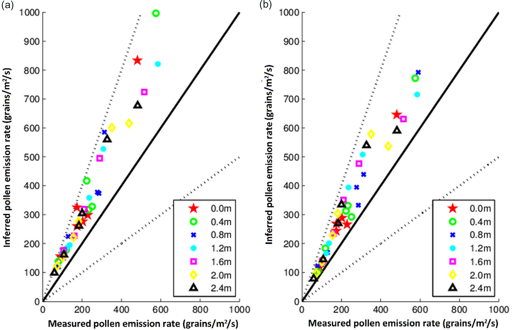
Fig. 6. Measured pollen emission rate versus inferred pollen emission rate (grains/m2/s) using the model at seven distances in the canopy gap showed only for (a) interaction 110 and (b) interaction 111 as defined in Table 1. The solid line is the one-to-one between observed and inferred pollen emission rates whereas the dotted lines correspond to factor of two (i.e., y = 0.5 × x and y = 2 × x).
Table 4. Summary of the four statistical performance parameters: the fractional bias (FB), the geometric mean bias (MG), the normalized mean square error (NMSE) and the geometric mean variance (VG) classed per interaction as defined in Table 1

Figure 7 shows the measured and inferred emission rates using the SMOP model for interactions 001, 110 and 111 as a function of time. Measured and inferred emission rates decreased with time and the inferred ones are higher than the measured ones. These profiles show the quality of the model parameterization for interaction 111. Furthermore, measured rates decrease with time and are ranged at 10:15 UTC from 590 grains/m2/s at 0.8 m to 438 grains/m2/s at 2.0 m, and at 12:45 UTC from 107 grains/m2/s at 1.6 m to 60 grains/m2/s at 2.4 m. However, the inferred emission rates, for interaction 110 (resp. 111), are ranged from 1022 to 615 grains/m2/s (resp. from 792 to 536 grains/m2/s) at 10:15 UTC, and from 224 to 138 grains/m2/s (resp. from 169 to 104 grains/m2/s) at 12:45 UTC. These profiles show also the quality of the model parameterization for interaction 111. Although the inferred pollen rates are higher than the measured ones, these results are similar to those found by Jarosz et al. (Reference Jarosz, Loubet, Durand, Foueillassar and Huber2005) and Marceau et al. (Reference Marceau, Saint-Jean, Loubet and Huber2012).

Fig. 7. Measured and inferred pollen emission rates (grains/m2/s) estimated using the restricted setting where our model includes no deposition on leaves, no resuspension and either taking both horizontal and vertical pollen fluctuations into account or only the vertical, which correspond to 110 and 111 interactions versus the interaction 001 as defined in Table 1.
Table 4 summarizes the SMOP model performance: all statistical measures presented in this table are based on measured v. inferred pollen deposition rates, the calculated values are mostly within the range of acceptable model performance for interactions 110 and 111 corresponding to the fact that the model includes no deposition on leaves, no resuspension, and taking (or not) into account horizontal pollen fluctuations. And as presented in Fig. 7, these two interactions are used to infer maize pollen emission rates. For the remaining interactions, the results are out of the desired ranges.
Discussion
The SMOP model has been evaluated in many experimental studies with various hybrids, for example, studies conducted in France at Montargis and Grignon in 2000–2002, 2008 and 2009 (Jarosz et al., Reference Jarosz, Loubet and Huber2004, Reference Jarosz, Loubet, Durand, Foueillassar and Huber2005; Marceau et al., Reference Marceau, Loubet, Andrieu, Durand, Foueillassar and Huber2011, Reference Marceau, Saint-Jean, Loubet and Huber2012). During these experiments, airborne concentration and deposition rates of maize pollen were measured at several locations within and downwind from various maize fields. All of these validations were done without a detailed sensitivity analysis of the model, such as that conducted in the current work, to pinpoint uncertainties in maize pollen deposition rates as well as in inference of pollen emission rates. Note that Jarosz et al. (Reference Jarosz, Loubet and Huber2004) and Marceau et al. (Reference Marceau, Saint-Jean, Loubet and Huber2012) carried out an SA of the model but only to the settling velocity, and showed that measured and modelled deposition rates performed at downwind distance x = 3 m and x = 10 m were very sensitive to this uncertain variable.
Using the surface wetness index measurements Jarosz et al. (Reference Jarosz, Loubet, Durand, McCartney, Foueillassar and Huber2003) and Marceau et al. (Reference Marceau, Saint-Jean, Loubet and Huber2012) have shown that the start of the pollen release in the morning appeared to coincide with the drying of the crop, and the largest concentration and deposition usually occurs at around 10:00 UTC (Scott, Reference Scott1970; Gregory, Reference Gregory1973; Marceau et al., Reference Marceau, Loubet, Andrieu, Durand, Foueillassar and Huber2011) which is the time when our experiment was done. Furthermore, Marceau et al. (Reference Marceau, Loubet, Andrieu, Durand, Foueillassar and Huber2011) and Sofiev et al. (Reference Sofiev, Siljamo, Ranta, Linkosalo, Jaeger, Rasmussen, Rantio-Lehtimaki, Severova and Kukkonen2013) have explored and quantified the effects of both meteorological variables and variety on pollen emission. Their data analysis revealed the effects of temperature and relative humidity on both diurnal and seasonal patterns of emission. The rate of pollen emission was higher when temperatures were high and lower when the humidity was high. In addition, they have shown that the pollen emission rate is higher when the wind speed is high. However, direct measurement of pollen release rate is not easy to quantify as this flux remains difficult to estimate. Jarosz et al. (Reference Jarosz, Loubet, Durand, McCartney, Foueillassar and Huber2003) and Marceau et al. (Reference Marceau, Loubet, Andrieu, Durand, Foueillassar and Huber2011) inferred the release rate by combining pollen measured directly on the tassel and deposition measured above the source using the slope of the linear regression.
In this study, the inferred pollen emission rate is calculated using Eqn (11) for only two validated interactions 110 and 111. However, before conducting this inference, we have to inspect the influence of environmental variables on the simulated pollen deposition rates by using a global sensitivity analysis. Table 2 shows that increasing the meanWS seems to increase the pollen deposition rate in the canopy gap; this may be explained by the fact that the horizontal wind speed in the canopy gap is low, and inertia and crossing trajectories effect of heavy particles is small (Snyder and Lumley, Reference Snyder and Lumley1971; Reynolds, Reference Reynolds2000). The same result is also shown for detailed sensitivity analysis by including interactions (Fig. 3 and Table 3). Nevertheless, turbulence intensity increases immediately downwind of a roughness change (Gash, Reference Gash1986) and, in particular, much more in a canopy gap. One can see that deposition rates decrease when the leaf area density, which is expressed in horizontal and vertical projections, increases. Indeed, when modelling pollen trajectories, not all of the pollen deposited on leaves and ground rebound. The global regression shows that SRC, NRC and LCC methods provide a different order of the more influenced variables on the simulated deposition rates (Table 2). This may be due to the discrete variables as well as to the variances of the inputs and the output pollen deposition rate, for example, the variance of LADz is equal to approximately 169 times the variance of StdWS; and the variance of LADx is equal to approximately 8 times the variance of meanWS. More accurately, SRC and NRC coefficients are related as follows.

where VXj and VY are the coefficients of variation for Xj and Y, respectively. This global sensitivity analysis showed that the real influence of each of the seven input variables on deposition rates cannot be concluded.
Jarosz et al. (Reference Jarosz, Loubet and Huber2004) have shown that for larger settling velocity the model simulates the deposition rates better near the source but does not simulate the concentration profiles correctly, especially at x = 10 m, where measured concentrations are greatly underestimated for large meanWS. These results suggest that discrepancies in concentration and deposition reported by the model near the source are unlikely to be solely due to pollen settling velocity. To better understand this discrepancy and since no definite results could be concluded from the global sensitivity analysis, eight combinations of the three 2-level variables were introduced. By considering these combinations, the SMOP model may be represented as a linear model, which is established by the coefficient of determination $R_{adj}^2$ (Table 3). Simulated pollen deposition rates are given in Figs 2 and 3, and the calculated values tended to be in the same range as those reported by Aylor et al. (Reference Aylor, Boehm and Shields2006). Figure 2 shows great variability of pollen deposition; furthermore, when the canopy and ground are perfect sinks (i.e., no pollen rebound on leaves and ground among 75% of the impacted pollen) and horizontal fluctuations are accounted for, the amount of pollen reaching the deposition cup will decrease almost to zero (deposition near zero). One could interpret that an effect of an increase of probability of impaction is due to increased particle horizontal velocity. This also explains the larger correlation coefficient of LADz in Fig. 4 for 001 when compared to 011. Meanwhile, the interactions 100 and 101 show positive correlations between deposition rate and LADz while all other combinations show negative correlations (Fig. 4). This is probably because the 100 and 101interactions correspond to maximum rebound on plants and ground while 110 and 111 have rebound only on the ground. This is the only situation for which the increase of LADz show an effect via lowering the wind speed profile in the canopy (which depends on LADz), while in any other case, the deposition by impaction dominates. In the literature, little information is known about pollen resuspension from either leaves or the ground. Aylor et al. (Reference Aylor, Schultes and Shields2003) have shown experimentally that pollen could be quite easily dislodged from maize leaves by either leaf shaking, roll-off or small wind speed (0.2–0.5 m/s). However, in the current experiment, the wind speed was fixed at 4.06 m/s which explain the neglected effect of 1D variable on the deposition rate.
Daily measured pollen emission rates and therefore deposition rates depend on the local weather conditions (e.g., Scott, Reference Scott1970; Gregory, Reference Gregory1973; Marceau et al., Reference Marceau, Loubet, Andrieu, Durand, Foueillassar and Huber2011). This explains the results given in Fig. 5: measured deposition rates are approximately unchangeable with distance in the canopy gap and do not decrease as is the case when we consider deposition rates downwind the source (Jarosz et al., Reference Jarosz, Loubet, Durand, McCartney, Foueillassar and Huber2003; Marceau et al., Reference Marceau, Loubet, Andrieu, Durand, Foueillassar and Huber2011; Torimaru et al., Reference Torimaru, Wennstrom, Lindgren and Wang2012). This result is certainly due to the turbulence intensity in the canopy gap and may explain the discrepancy between measured and simulated pollen deposition rates (Figs 6 and 7). Indeed, the empirical parameterization of turbulence field in the transition zone used is not the correct one and future versions of the model should take this conclusion into account.
Variations in input variables (Fig. 7) have a large effect on the inferred pollen emission rates. Dupont et al. (Reference Dupont, Brunet and Jarosz2006) showed that a simplified parameterization of turbulence in the area between two different canopies leads to underestimates of pollen deposition close to the field. However, the current work found the opposite, i.e. the simulated pollen deposition rates overestimate the measured ones (Figs 6 and 7). The meteorological conditions during these experiments were not reported in sufficient detail to draw definite conclusions about quantities of maize pollen released and distance of pollen dispersal in the canopy gap. Various assumptions are cited below to explain this overestimation:
(1) the surface is dynamically heterogeneous that could perhaps lead to overestimation of the turbulence intensity in the canopy gap (Flesch et al., Reference Flesch, Wilson and Yee1995): larger turbulence intensity would induce larger vertical diffusion, which favours larger deposition rates near the source. Indeed, it is difficult to describe correctly the turbulence flow in the transition zone at the downwind edge of the source and in particular in a canopy gap (Gash, Reference Gash1986; Heisler and DeWalle, Reference Heisler and DeWalle1988; McCartney and Lacey, Reference McCartney and Lacey1991). They showed that, immediately downwind of a roughness change, the turbulence intensity increases three times over normal conditions. By taking into account these results, the SMOP model includes an empirical parameterization of the turbulence field for heterogeneous landscapes. However, this parameterization, which was also used in the current simulation, is possibly not valid for the canopy gap that is established by an approximately constant deposition rate with distance (Fig. 5),
(2) by considering interactions 110 and 111, i.e. where there is no deposition on leaves and no rebound of pollen, the variable meanWS is the only significant variable (Fig. 3); therefore, lower meanWS leads to less deposition. The settling velocity, as well as many of the biophysical characteristics of pollen, is mainly determined by pollen water content (Di-Giovanni et al., Reference Di-Giovanni, Kevan and Nasr1995; Aylor, Reference Aylor2003; Loubet et al., Reference Loubet, Jarosz, Saint-Jean and Huber2007; Marceau et al., Reference Marceau, Saint-Jean, Loubet and Huber2012). Indeed, pollen water content affects pollen mass, diameter and density which determine pollen settling velocity as formulated by Di-Giovanni et al. (Reference Di-Giovanni, Kevan and Nasr1995). In the current work, the simple model proposed by Marceau et al. (Reference Marceau, Saint-Jean, Loubet and Huber2012) was used to predict accurately pollen water content at emission as a function of air vapour pressure deficit. In our opinion, this simple model computes with uncertainty pollen water content, which affects the pollen settling velocity. Hence, the overestimation of the deposition rate would be linked to an erroneous parameterization of intervals of the two variables describing the Gaussian distribution of pollen settling velocity,
(3) biased emission and deposition rates measurements; the cups used to collect the pollen grains influence their deposition on the ground. McCartney and Lacey (Reference McCartney and Lacey1991) showed experimentally that numbers of spores collected on horizontal microscope slides openly exposed were almost double to those on slides placed on a table or at the bottom of large cups. Hence, collecting pollen in containers could have led to an underestimation of the deposition rate in the current work (McCartney et al., Reference McCartney and Lacey1991), and
(4) the quantity of pollen deposited in the source itself was estimated to range from 17 to 50% (Jarosz et al., Reference Jarosz, Loubet and Huber2004). Then, by taking into consideration interactions 110 and 111 where there is no pollen deposition on leaves, the simulated deposition rates automatically overestimate the measured deposition ones in the canopy gap.
The real pollen emission rate at a given time is always difficult to determine. To this end, one should use the inference methodology set out in the current paper for calibration of the parameters by combining the Lagrangian stochastic model with a high-resolution version of the meteorological flow model, if they have to be used in complex experiments. Without any calibration of the model as detailed in this work, the inference of pollen emission rate appears to be uncertain.
Conclusion
The current study has shown that the inferred emission rate overestimates the measured quantities. Sensitivity Analysis has shown that simulated pollen deposition rates are mainly influenced by and correlated with the mean gravitational settling velocity and to the leaf area density. The overestimated emission rate could possibly be as a result of (i) biased emission and deposition rates measurements, (ii) gravitational settling velocity of pollens, (iii) pollen deposition on leaves or pollen resuspension from the leaves or the ground. However, the model overestimation of the emission rate could also be due to a parameterization of the turbulent field in the canopy gap.
Financial support
This research received no specific grant from any funding agency, commercial or not-for-profit sectors.
Conflicts of interest
The authors declare no conflicts of interest exist.
Ethical standards
Not applicable.


