


Introduction
Global population growth is determining a progressive increase of the demand for food supply, which in turn increases the amount of water that needs to be allocated for crop production. In some areas of the world, irrigated agriculture represents the major consumer of water resources, typically about 0.70 of the total water use (UNWAP 2016). Indeed, irrigation allows lands to be, on average, twice as productive as rain-fed lands. In areas such as southern Mediterranean regions, irrigation is essential for ensuring high crop yields during late spring and summer, characterized by high temperatures and lack of rain (Wriedt et al. Reference Wriedt, Van der Velde, Aloe and Bouraoui2009).
Improving the efficiency of water use for irrigation is required for ensuring long-term sustainability of irrigated agriculture (Pereira et al. Reference Pereira, Cordery, Iacovides, Pereira, Cordery and Iacovides2009). The EU Common Agricultural Policy, combined with the Water Framework Directive, imposes a substantial increase in the efficiency of water use in agriculture for the next decades on farmers and irrigation managers (Heinz Reference Heinz2008).
The strategies for more rational and efficient water consumption in agriculture may be categorized as policy, engineering, system and irrigation/agronomic practice interventions (Stöckle Reference Stöckle2001). Among the latter interventions, one possible solution is to irrigate according to reliable estimates of actual water that must be supplied by irrigation to satisfy crop water needs, which are not provided by rainfall or by water available in the profile (Romano et al. Reference Romano, Palladino and Chirico2011).
For this purpose, irrigation advisory services have been built to help farmers decide the right amount of water to be supplied. These services provide an assessment of the crop water requirement (CWR) to farmers, accounting for the meteorological conditions and the development stage of the crop. The effectiveness of these CWR estimates relies on the availability of updated data about the crop and the meteorological conditions, with adequate spatial and temporal resolution (Allen et al. Reference Allen, Pereira, Howell and Jensen2011).
Current Earth observation (EO) systems provide multispectral imagery of crops with relatively high spatial and temporal resolutions. Several models have been developed and successfully applied to exploit the available time series of visible and near-infrared (VIS-NIR) images of the crop for estimating crop potential evapotranspiration (ETp) and crop water use. The main space agencies, such NASA and ESA, provide georeferenced multispectral imagery with a high spatial resolution (30 m or less) and small time intervals (9 days or less), free of charge. This data policy enhanced the development of satellite-based services that can offer irrigation advice to farmers at a reasonable cost. A review of the current application of remote sensing for crop water management has been provided recently by Calera et al. (Reference Calera, Campos, Osann, D'Urso and Menenti2017).
In southern Mediterranean regions, ETp is the main component of CWR, under the assumption that irrigated crops grow under excellent agronomic and soil water conditions (Allen et al. Reference Allen, Pereira, Raes and Smith1998). One possible approach for estimating ETp is to apply the Penman–Monteith equation, with crop parameters estimated from remotely sensed images. This is the so-called ‘one-step’ approach followed by some satellite irrigation services, such as IRRISAT in Southern Italy (https://www.irrisat.com/en/), EO4Water in Lower Austria (https://eo4water.com/) and IRRIEYE in Southern Australia (http://www.irrieye.com).
In addition to crop parameters, the Penman–Monteith equation needs meteorological data as input variables, including air temperature, wind speed, solar radiation and relative humidity. These data are often unavailable or available only with large uncertainty, since they are estimated by spatial interpolation of sparse meteorological ground stations. The reliability of meteorological data produced by numerical weather prediction (NWP) models has improved considerably in the 21st century. Thus, NWP model outputs are a valuable source for estimating the meteorological variables relevant for calculating ETp maps, alternative to the spatial interpolation of spatially coarse ground-based weather data sets (WMO 2012).
Operational NWP models can be also exploited for forecasting ETp a few days ahead. This is particularly relevant for providing irrigation advice to farmers in operative scenarios, since it allows planning of irrigation water supply based on the expected meteorological conditions rather than on past and current meteorological data.
The current study presents an innovative ETp forecasting system that has been implemented recently in the Campania region (southern Italy). The forecasting system has been integrated into the IRRISAT irrigation advisory service, which has been operative in the Campania region since year 2007 and was originally based on remote-sensing crop imagery and ground-based meteorological data. The new forecasting system integrates high-resolution numerical weather forecasts with VIS-NIR crop imagery for providing ETp maps to farmers with a lead time of 5 days. The current paper presents the methodological background and key operational settings of the forecasting system. The forecast performance of crop ETp was evaluated at two experimental sites in Campania region, by comparing the forecasted ETp with that estimated by means of ground meteorological observations.
Materials and methods
Methodological background for crop potential evapotranspiration assessment
The CWR can be estimated according to the standard approach proposed by Allen et al. (Reference Allen, Pereira, Raes and Smith1998):
 $${\rm CWR = E}{\rm T}_{\rm p} - P_{\rm e}$$
where ETp (mm) is the crop potential evapotranspiration, i.e. the amount of water consumed by crops via soil evaporation and plant transpiration under optimum soil water conditions, and P e (mm) is the effective precipitation, i.e. the part of the rainwater effectively available for crops, namely the rainwater excluding the losses due to run-off and foliage interception.
During the irrigation season in southern Italy, due to features of the Mediterranean climate, rainfall events are rare and generated generally by intense thunderstorms of short duration and small spatial extent, highly influenced by the local topography (Furcolo et al. Reference Furcolo, Pelosi and Rossi2016). These rainfall patterns make monitoring difficult with traditional rain gauge networks (Zoccatelli et al. Reference Zoccatelli, Borga, Chirico and Nikolopoulos2015), and forecasting with current NWP models is highly uncertain (Montani et al. Reference Montani, Cesari, Marsigli and Paccagnella2011). These characteristics of summer and spring have been enhanced by the climatic change observed in the last century (Diodato et al. Reference Diodato, Bellocchi, Romano and Chirico2011). Such rainfall events may cause floods at local scale but provide little water supply to open field crops (Preti et al. Reference Preti, Forzieri and Chirico2011). Thus, the rainfall contribution to overall CWR is generally negligible as compared with crop ETp (D'Urso Reference D'Urso2010).
Potential evapotranspiration depends on both crop parameters, such as surface albedo and crop height, and weather variables, such as air temperature, solar radiation, humidity, wind speed and air pressure.
One conventional approach for assessing ETp is the so-called ‘two-steps’ procedure recommended by Allen et al. (Reference Allen, Pereira, Raes and Smith1998). According to this procedure, ETp can be evaluated by multiplying the reference evapotranspiration (ET0) with a crop coefficient (K c).
The reference evapotranspiration is the potential evapotranspiration of a hypothetical grass reference crop under optimum soil water conditions and can be calculated with the FAO Penman–Monteith equation using only weather information:
 $${\rm E}{\rm T}_{\rm 0} = \displaystyle{{\rm 1} \over \lambda} \displaystyle{{\it \Delta {\rm (}R_{\rm n} - G{\rm )} + \gamma {\rm (900/}T + {\rm 273)}U{\rm (}e_{\rm s} - e_{\rm a}{\rm )}} \over {\it \Delta + \gamma {\rm (1} + {\rm 0}{\rm {\cdot}34}U{\rm )}}}$$
where λ is the latent heat of vaporization of water (MJ/kg), R n is the net radiation at the crop surface (MJ/m2/day), G is the soil heat flux density (MJ/m2/day), T is the daily mean air temperature at 2 m height (°C), U is the wind speed at 2 m above the ground (m/s), e s is the saturation vapour pressure (kPa), e a is the actual vapour pressure (kPa), Δ is the slope of the vapour pressure curve (kPa/°C) and γ is the psychometric constant (kPa/C).
The crop coefficient is then a proxy of the parameters describing the canopy development, i.e. leaf area index (LAI), surface albedo and crop height (Vuolo et al. Reference Vuolo, D'Urso, De Michele, Bianchi and Cutting2015).
An alternative method, which is the one used by IRRISAT for producing remote-sensing-based estimates of ETp, is the so-called ‘one-step’ approach (D'Urso & Menenti Reference D'Urso, Menenti, Engman, Guyot and Marino1995) that explicitly employs aerodynamic and surface resistances to compute ETp as follows:
 $${\rm E}{\rm T}_{\rm p} = \displaystyle{{{\rm 86400}} \over \lambda} \left[ {\displaystyle{{\it \Delta {\rm (}R_{\rm n} - G{\rm )} + \rho c_{\rm p}^{} {\rm (}e_{\rm s} - e_{\rm a}{\rm )}/r_{\rm a}} \over {\it \Delta + \gamma {\rm (1} + r_{\rm s}/r_{\rm a}{\rm )}}}} \right]$$
where ρ is the mean air density at constant pressure (kg/m3), c p is the specific heat of the air (MJ/kg/°C), r a and r s are the aerodynamic and surface resistances, respectively (s/m).
Visible and near-infrared imagery are processed to estimate the canopy parameters required for applying Eqn (3): LAI, crop height (h c) and the hemispherically integrated albedo (r).
The variability of LAI during the phenological development of the crop has the largest impact on the estimation of ETp, as compared with r and h c (Vanino et al. Reference Vanino, Pulighe, Nino, De Michele, Falanga Bolognesi and D'Urso2015).
Leaf area index and h c are used for computing the aerodynamic and surface resistances:
 $$r_{\rm a} = \displaystyle{{{\rm ln[2}{\rm -} {\rm 2/3}h_{\rm c}/{\rm 0}{\rm {\cdot}123}h_{\rm c}{\rm ]ln[2}{\rm -} {\rm 2/3}h_{\rm c}/{\rm 0}{\rm {\cdot}0123}h_{\rm c}{\rm ]}} \over {{{\rm (0}{\rm. 41)}}^{\rm 2}U}}$$
 $$r_{\rm s} = \left\{ \matrix{\displaystyle{{{\rm 200}} \over {{\rm LAI}}}\quad \forall {\rm LAI} \le 4 \hfill \cr {\rm 50}\quad \quad \forall {\rm LAI} \gt 4 \hfill} \right.$$
Albedo is used to estimate the fraction of incoming short-wave radiation contributing to the net radiation R n.
IRRISAT operationally exploits LANDSAT-8 VIS-NIR imagery for estimating canopy parameters with a spatial resolution of 30 m. Upgrades are planned to exploit the Sentinel-2 remote-sensing imagery with a spatial resolution of 10 m.
The surface reflectance is used to estimate LAI with the CLAIR model (Clevers Reference Clevers1989):
 $${\rm LAI =} {\rm -} \displaystyle{1 \over \alpha} {\rm ln}\left( {1 - \displaystyle{{{\rm WDVI}} \over {{\rm WDV}{\rm I}_\infty}}} \right)$$
where α is a shape parameter that must be calibrated with LAI field measurements, WDVI is the weighted difference vegetation index and WDVI∞ is the asymptotic value for LAI → ∞, and it is computed from the spectral reflectance (Vuolo et al. Reference Vuolo, Neugebauer, Bolognesi, Atzberger and D'Urso2013).
Given the limited spectral resolution of the VIS-NIR imagery employed, albedo is calculated as a weighted sum of surface spectral reflectance:
 $$r = \sum\limits_{\lambda = {\rm 1}}^n {\rho _\lambda w_\lambda} $$
where ρ λ is the surface spectral reflectance derived from the atmospheric correction, while w λ is the fraction of solar irradiance in each sensor band, according to D'Urso & Calera Belmonte (Reference D'Urso and Calera Belmonte2006).
Crop height can be derived from crop maps or as function of LAI with a specific regression equation that needs to be empirically determined. When this information is not available, h c is fixed to 0.4 m. This is an acceptable approximation since the variability of crop height h c has little impact on the value of ETp, especially in southern Mediterranean regions where the aerodynamic term of the FAO Penman–Monteith equation is much smaller than the corresponding radiative term (Vuolo et al. Reference Vuolo, D'Urso, De Michele, Bianchi and Cutting2015).
Numerical weather forecasts
The new ETp forecasting system implemented by IRRISAT adopts the NWP outputs provided by COSMO-LEPS, which is a Limited Area Ensemble Prediction System, operated by the HydroMeteoClimate Regional Service of Emilia-Romagna, located in Bologna, Italy (ARPA–SIMC). Pelosi et al. (Reference Pelosi, Medina, Villani, D'Urso and Chirico2016) showed that COSMO-LEPS produces skilful and reliable forecasts of the weather variables relevant for reference evapotranspiration (ET0) estimates in Campania region, up to 5 days ahead, with limited sensitivity to the forecast lead time.
Since December 2011, COSMO-LEPS has run twice a day, at 00:00 UTC and 12:00 UTC. The model has a forecast range of 132 h, with data available at 3 h intervals and a spatial resolution of 7.5 km. The relevant weather variables to calculate ETp are extracted from GRIB (GRIdded Binary or General Regularly-distributed Information in Binary form) files released as output of the 00:00 UTC run: atmospheric pressure reduced to mean sea level, net short-wave radiation, albedo, wind speed at 10 m above ground level, temperature and relative humidity at 2 m. Figure 1 shows the points of the numerical grid adopted by COSMO-LEPS covering the Campania region.

Fig. 1. COSMO-LEPS numerical grid (red circles) over Campania region and location of Improsta and Soffritti farms hosting the verification sites.
The numerical weather forecasts at a specific site are retrieved by a triangle-based bi-linear interpolation method, which consists of interpolating the three numerical grid points closest to the examined site. A statistical post-processing technique is applied for partially removing systematic and non-systematic forecast errors produced by the NWP models, when ground measurements of weather variables are available (Pelosi et al. Reference Pelosi, Medina, Van den Bergh, Vannitsem and Chirico2017).
Web2.0 service for delivering crop potential evapotranspiration forecast maps
Farmers can access ETp forecast maps by means of a dedicated web-based platform with a protected login. At first access, farmers need to draw the boundary of plots for which they request the advisory service on a base layer. The platform then displays updated maps and time series of crop LAI and daily crop evapotranspiration, with a forecast horizon up to 5 days, beside other variables of potential interest for the farmer (e.g. air temperature, rainfall, etc.). By clicking on the maps, the platform displays the time series of the corresponding variables, either for each selected pixel or aggregated at plot scale, according to the user requirement.
Sample layouts of the windows dedicated to LAI and crop ETp are displayed in Figs 2 and 3. The web layouts are made up of a coloured map with a legend, and graphs displaying both the current value and the time series of the selected variable. In case of ETp time series, the graph provides the values 5 days ahead of the current day. Users can move the map by keeping the mouse button held down while dragging it, and can use the zoom in and zoom out button in the top left corner of the map. For touchscreen devices, users can also use the multi-touch gesture to pan and zoom the map. The position button, on the bottom left, displays your location (based on global position system (GPS) device of tablet or smartphone) on the map. Data in tabular format are also provided as a summary report.

Fig. 2. Layout of the web-based app, displaying LAI map and time series at a farm plot: a coloured map with legend is located at the top. The graph at the bottom left displays the LAI value at the current day. On the bottom right, the graph displays the time series of the LAI.
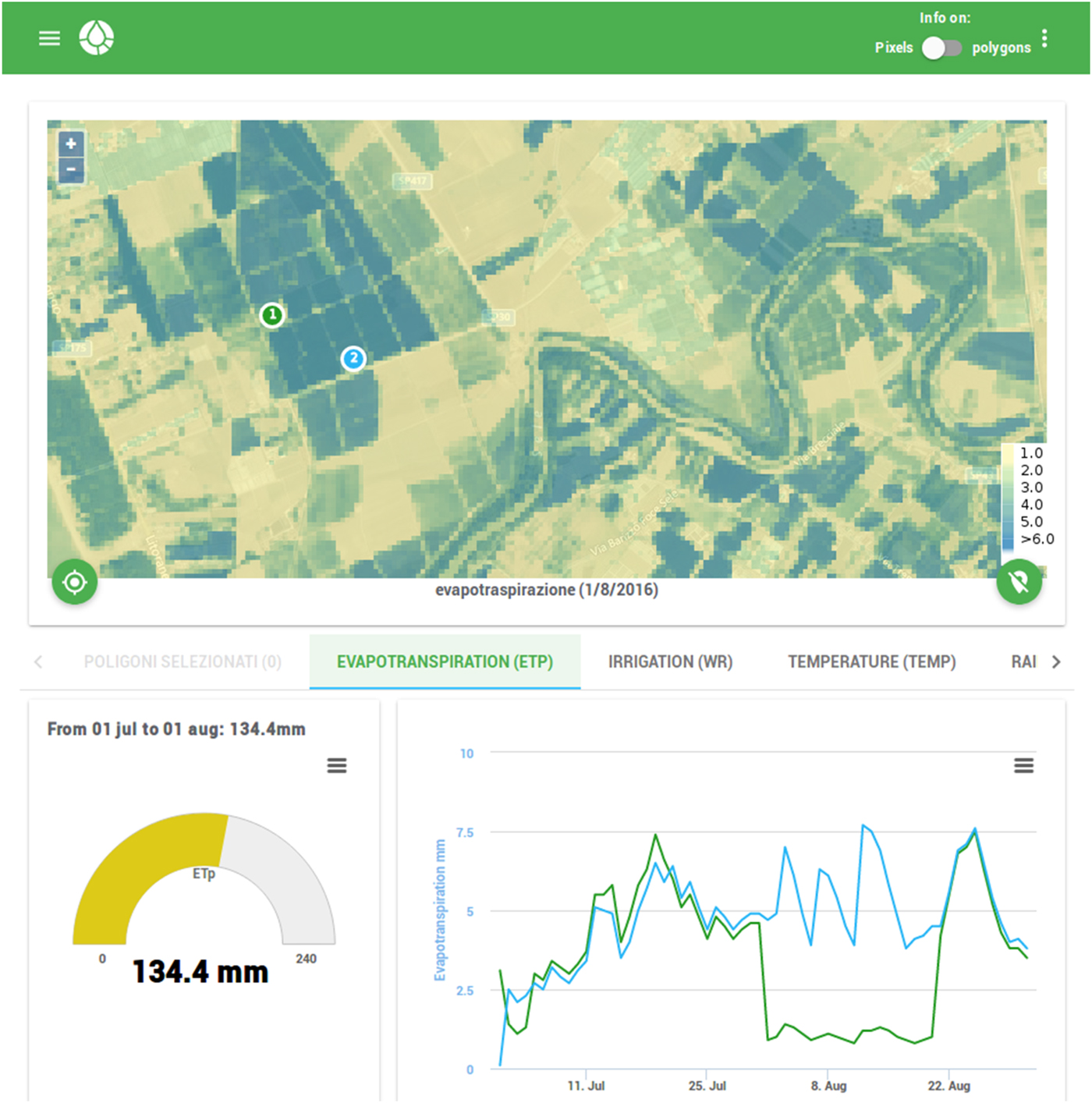
Fig. 3. Layout of the web-based app, displaying crop ETp map and time series at a farm plot: a coloured map with legend is located at the top. The graph at the bottom left displays the cumulative ETp with a user-defined time interval. On the bottom right, the graph displays the time series of the cumulative ETp.
Measurements at the experimental maize fields
The test sites consisted of maize crop fields hosted by two farms, Soffritti (40°27′) and Improsta (15°1′), located in the Campania region (Fig. 1). Under the Köppen–Geiger climate classification, this region is characterized by dry-summer sub-tropical climates, which are often referred to as Mediterranean climate. During summer, the mean monthly temperature ranges from 25 to 30 °C and during winter, between 11 and 17 °C. The precipitation patterns are influenced strongly by the interaction of wet air masses with the orography (Pelosi & Furcolo Reference Pelosi and Furcolo2015): mean annual precipitation ranges from 800 to 1100 mm. The maximum monthly precipitation values are recorded during November and December, minimum values during July and August. Irrigation in open fields starts no earlier than April and lasts until the end of September, although the actual time span of the irrigation season is influenced by climatic fluctuations and specific agricultural practices.
The two selected farms are representative of two different topographic conditions: Improsta is located in a large floodplain; Soffritti is located in a hilly inland area. Choosing different terrain is relevant for evaluating ETp forecast performances, since local topographic conditions significantly affect the reliability of the numerical weather forecast, as in other coastal regions of the central Mediterranean basin (Buzzi et al. Reference Buzzi, Fantini, Malguzzi and Nerozzi1994), as well as of satellite-based estimations of LAI (Calera et al. Reference Calera, Campos, Osann, D'Urso and Menenti2017).
Each farm was equipped with ground-based automatic weather stations (AWS) providing measurements of precipitation, atmospheric pressure, solar radiation, relative humidity, wind speed at 10 m above ground level and temperature at 2 m, with high accuracy and precision standards.
Ground LAI measurements were taken as follows: from seven fields at Improsta on two dates in 2014, simultaneously to DEIMOS-1 satellite acquisitions; from six fields at Soffritti farm on eight dates in 2015, some of them close to or at the same time as LANDSAT-8 Operational Land Imager (OLI) satellite acquisitions.
Ground non-destructive measurements of LAI and leaf mean tilt angle were made with a LICOR LAI-2000 Plant Canopy Analyser (LI-COR 1992), which works by comparing the intensity of diffuse incident illumination measured at the bottom of the canopy with that arriving at the top. In order to reduce the effect of multiple scattering on LAI-2000 measurements, the instrument was only operated near dusk and dawn (6:30–9:30 a.m.; 6:30–8:30 p.m.) under diffuse radiation conditions, using one sensor for both above- and below-stand measurements. In order to prevent interference caused by the operator's presence and the illumination conditions, the sensor field of view was limited using a 180° view cap. Measurements were azimuthally oriented opposite to the sun azimuth angle. Leaf area index measurements were taken with the instrument held a few centimetres above the soil, generally within 3 days of image data acquisition. A measurement of ambient light was made with the sensor extended upward and over the top of the canopy at arm's length. Eight below-canopy readings were then made. This procedure was conducted three times per spot, and the resulting 24 samples comprise one full set of measurements. Finally, each centre of the LAI-2000 transects was geolocated using GPS measurements. This measurement protocol allowed determination of statistically meaningful LAI values, characterized by a low ratio between the standard error of the LAI (SEL) and LAI itself (SEL/LAI ranged between ≈0.03 and ≈0.13 for the test sites at Improsta and SEL/LAI ranged between ≈0.02 and ≈0.17 for the test sites at Soffritti); thus, the actual LAI should be within 11% of the LAI sample mean.
Leaf area index maps at Improsta were derived by combining DEIMOS-1 satellite acquisitions with a spatial resolution of 22 m and LANDSAT-8 imagery, to get LAI data with an average time frequency of 1 week. Leaf area index maps at Soffritti were derived with a spatial resolution of 30 m from LANDSAT-8 imagery elaborated with a time frequency of 15 days, allowing for favourable atmospheric conditions.
DEIMOS-1 is a commercial tasking EO satellite and is part of the Disaster Monitoring Constellation (DMC) (http://www.dmcii.com). The sensor records radiance in three spectral bands corresponding to green (520–600 nm), red (630–690 nm) and near-infrared (770–890 nm) parts of the electromagnetic spectrum at a ground sampling distance (GSD) of 22 m. DEIMOS-1 images were processed to a high degree of accuracy using an industry-standard atmospheric correction algorithm (ATCOR-2) (Richter Reference Richter1996; GEOSYSTEMS 2017).
LANDSAT-8 OLI data at a GSD of 30 m were generated routinely by the Landsat Ecosystem Disturbance Adaptive Processing System (LEDAPS) and obtained through the USGS Land Science Research and Development (LSRD) website; LEDAPS uses Dense Dark Vegetation (DDV) targets to estimate the aerosol optical thickness (AOT). The estimated AOT was used afterwards as input to the Second Simulation of a Satellite Signal in the Solar Spectrum (6S) radiative transfer model.
All images were elaborated using Eqn (6) with α = 0.35, which was determined for this area based on previous field campaigns (D'Urso & Calera Belmonte Reference D'Urso and Calera Belmonte2006).
Results
Satellite-based estimates of leaf area index
In total, 62 ground LAI measurements (seven fields per two dates at Improsta and six fields per eight dates at Soffritti) were taken during the two irrigation seasons 2014 and 2015. The satellite estimations were in good agreement with the ground observations (coefficient of determination R 2 = 0.70). Figure 4 shows the scatterplot of field and satellite LAI estimates of years 2014 and 2015 at the test sites.

Fig. 4. Scatter plot of satellite estimates of LAI v. field estimates of LAI at Improsta and Soffritti farms. The red line is the 45-degree line of perfect agreement between the two estimates; the green dashed line is the least-squares line computed from data. The R 2 statistics refers to the perfect agreement between the two data sets.
Figure 5 shows the time evolution of satellite and field LAI estimates at the three test fields at Improsta and Soffritti, respectively. The data show good agreement in the central part of the irrigation season, while larger differences are observed in the second half of July. A systematic overestimation of LAI by satellite was observed at some plots in Soffritti. The impact of these differences on ETp forecasts was generally negligible, especially for high LAI values, given the asymptotic behaviour of Eqn (3).

Fig. 5. Time evolution of LAI estimates from satellite images and ground measurements at three of the selected maize fields of Improsta farm (top row) and Soffritti farm (bottom row).
Potential evapotranspiration prediction errors obtained by applying Eqn (3) with LAI equal to the one estimated with the last satellite acquisition were generally larger than those obtained by applying Eqn (3) with LAI estimated by remote-sensing, especially in the central part of phenological development of the crop.
Crop potential evapotranspiration forecasts
The performances of the new ETp forecasting system implemented in IRRISAT at the selected fields are presented. The ‘best estimate’ of ETp, taken as a benchmark to assess the forecast performances, was computed by using ground-based weather data combined with interpolated values of LAI between two satellite estimates. The IRRISAT approach used COSMO-LEPS forecasts for weather variables and LAI equal to the last available satellite estimate, to provide forecasts of ETp with a lead time of up to 5 days.
The performance analysis also included a ‘mixed approach’, which used COSMO-LEPS weather forecasts and interpolated values of LAI between two satellite estimates, to evaluate the impact of IRRSAT LAI approximation on ETp forecasts. Table 1 provides a summary of the methods employed in this comparison study.
Table 1. Overview of the methods employed in the performance analysis

Figure 6 shows a sample temporal evolution of the 5-day cumulative ETp with lead time of 5 days as predicted by IRRISAT, in comparison with the best estimate and the estimate given by the mixed approach (COSMO + interpolated LAI), at two representative test sites located, respectively, at Improsta (left panel) and Soffritti (right panel). The IRRISAT and mixed approaches provided very similar estimates at Improsta in 2014 because of the high frequency of available satellite estimates of LAI. The main reason for dissimilarity between IRRISAT estimates and the best estimates is due to errors in the weather forecasts: on average, IRRISAT underestimates the 5-day cumulative ETp. On the contrary, at Soffritti in 2015, IRRISAT overestimated the 5-day cumulative ETp compared with the best estimate. Then, in this case, because of less frequent available satellite estimates of LAI, the differences between the estimates given by IRRISAT and mixed approaches were more evident and, as expected, IRRISAT underestimated the 5-day cumulative ETp with respect to the results of the mixed approach. The main sources of error in forecasting ETP were still due to errors in the weather forecasts, although errors due to LAI approximations were not negligible.

Fig. 6. Sample time series of 5 days accumulated ETp forecasted with a lead time of 5 days by means of the IRRISAT approach and the mixed approach, based on post-processed COSMO-LEPS outputs. The forecasted values are compared with the best estimate obtained by employing measured weather data.
Figures 7(a) and (b) depict the BIAS and RMSE, respectively, of the cumulative ETp forecast by IRRISAT with respect to the best estimate. The boxplots show the BIAS and RMSE across all test sites, belonging to the two different farms, for increasing cumulative forecasting time intervals (1, 3 and 5 days). On each box, the central mark is the median, the edges of the box are the 25th and 75th percentiles, the whiskers extend to the most extreme data values not considered outliers, and outliers are plotted individually. The points are drawn as outliers if they are larger than q 3 + 1.5(q 3–q 1) or smaller than q 1 − 1.5(q 3–q 1), where q 1 and q 3 are the 25th and 75th percentiles, respectively. The circle mark represents the mean value among all test sites in the same farm.

Fig. 7. (a) BIAS (mm) and (b) RMSE (mm) of forecasted ETp accumulated in 1, 3 and 5 days for increasing lead time.
At Improsta, there was a prevailing negative BIAS, which means that IRRISAT on average underestimated the cumulative ETp. At Soffritti, the BIAS was on average positive, indicating overestimation. Table 2 summarizes the average BIAS and RMSE of the forecast ETp for different lead times (i.e. 1, 3 and 5 days) at both Improsta and Soffritti farms. The RMSE values were higher for the field sites at Soffritti than those at Improsta, probably because of the combined effect of the errors in weather forecasts and in the LAI approximations, as mentioned above.
Table 2. Summary of the average performance statistics of IRRISAT cumulative ETp forecasts with respect to the best estimate

The ratio, rBIAS, between the bias in ETp due only to the approximations made on LAI and the bias in ETp due only to weather forecasts, is defined as follows:
 $${\rm rBIAS} = \displaystyle{{\sum\nolimits_{i = 1}^n {\left \vert {{\rm ET}_{\rm p}^{{\rm IRRISAT}} {\rm -} {\kern 1pt} {\rm ET}_{\rm p}^{{\rm MIXED}}} \right \vert}} \over {\sum\nolimits_{i = 1}^n {\left \vert {{\rm ET}_{\rm p}^{{\rm MIXED}} {\rm -} {\kern 1pt} {\rm ET}_{\rm p}^{{\rm BEST}}} \right \vert}}} $$
where n is number of days in the irrigation season.
Figure 8 shows rBIAS across all test sites, belonging to the two different farms, for varying cumulative intervals having increasing lead times (1, 3 and 5 days). Table 2 reports the average rBIAS for different forecast lead times and at both Improsta and Soffritti farms.

Fig. 8. Ratio between the ETp absolute bias due to LAI approximations and the ETp absolute bias due to weather forecast errors.
The ratio rBIAS was always lower than unity, which means that, for the ETP forecasts, the main source of error is given by weather forecasts. It was higher at Soffritti than Improsta because of the less frequent available satellite LAI estimates (Fig. 5), which led to major approximations on LAI values. The variability of rBIAS with the lead time indicates that for Improsta, the impact on forecast errors of the approximations made on LAI increased with the cumulative time interval. For the case of Soffritti, this was valid only for rBIAS related to the 5-day cumulative ETp.
Discussion
Irrigation advisory services can take advantage of the latest generation of high-resolution NWP models, also known as limited area models (LAM), which represent a good data source for retrieving the weather data relevant for ETp estimation where the spatial density of weather stations is poor. These models also provide reliable forecasts of weather variables a few days in advance and with a spatial resolution of a few kilometres. In contrast, quantitative forecast of rainfall patterns is still affected by large uncertainty, especially for forecasting lead times longer than 24 h.
The current paper presents the performance of an innovative system providing forecasts of crop ETp with a lead time of 5 days, which has been implemented in the IRRISAT irrigation advisory service in Campania region (southern Italy). The forecasting system takes advantage of EO-imagery for assessing crop canopy parameters and a high-resolution NWP model for forecasting weather variables. It combines LAM outputs with a post-processing procedure of the crop VIS-NIR imagery, for computing maps of crop ETp based on the Penmann–Monteith equation. Other irrigation services, such as the Irrigation Water Management by Satellite and SMS system (IrriSatSMS) currently implemented in Australia, exploit the NWP model, but they implement the so-called FAO-56 two-steps procedure (Hornbuckle et al. Reference Hornbuckle, Car, Christen, Stein and Williamson2009). In IrriSatSMS, for example, NWP model outputs are used for forecasting reference crop evapotranspiration (ET0). Earth observation-imagery is then exploited for computing the basal crop coefficient, which is used to scale the forecast ET0 according to the specific crop phenological state.
Performances of the proposed ETp forecasting system were evaluated at two farms in the Campania region, located in areas characterized by significantly different topographic conditions. Potential evapotranspiration forecasts accumulated over 5 days were delivered 5 days in advance with an RMSE <3 mm (i.e. 0.6 mm/day) and an absolute bias <2 mm (i.e. 0.4 mm/day). Local terrain properties greatly affected both reliability of the weather forecasts and accuracy of the canopy parameters estimated from satellite images. In hilly and mountainous areas, weather forecasts are more prone to errors since numerical models (having a spatial resolution of a few kilometres) are not able to resolve the terrain effects on local weather patterns. Complex terrain features also represent a detrimental factor for post-processing satellite images (Moran et al. Reference Moran, Inoue and Barnes1997). For this reason, ETp forecast performances at Soffritti, which is located in a hilly area, were generally worse than at Improsta, located in a large river plain.
Another source of error for ETp forecasts lies in the fact that crop parameters are updated only when a new satellite image of the crop is available. This means that the accuracy of ETp forecasts is influenced by the frequency of satellite acquisitions, especially during the stages of fast crop canopy development. In the current study, the impact of this approximation on the ETp forecast was lower than that of the weather forecast errors. Nevertheless, the new EO systems, such as Sentinel-2, can contribute towards lessening the impact of this approximation by providing crop imagery with a smaller repeat cycle. Another option for dampening this source of error is to develop methods for forecasting the crop parameters (Medina et al. Reference Medina, Romano and Chirico2014a). For instance, crop models emulating the dynamic evolution of crop parameters could be implemented by sequentially assimilating the observations provided by satellite images (Chirico et al. Reference Chirico, Medina and Romano2014; Medina et al. Reference Medina, Romano and Chirico2014b).
Besides the valuable forecasting performances, the success of an irrigation advisory service also relies on its usability. For this reason, the new ETp forecasting system has been integrated with the most advanced web 2.0 technologies to deliver irrigation advice to farmers in an effective and intuitive format. Future studies will be devoted to evaluating the performance of the proposed irrigation advisory service from the end-users’ perspective.
Acknowledgements
The study is part of the PIRAM project, funded by the European Union and Campania region, within the rural development programme 2007–2013. COSMO-LEPS forecasts were provided by ARPA Emilia Romagna – Servizio Idro-Meteo-Clima. Improsta and Soffritti farms kindly permitted the execution of ground measurements.


