Introduction
Climate change impacts on agriculture and their implications for crop production are increasingly becoming the main themes of many case studies. These studies often emphasize that water may become one of the principal limiting factors for crop production in many areas (Blum Reference Blum2005; Trnka et al. Reference Trnka, Hlavinka, Semerádová, Dubrovský, Žalud and Možný2007, Reference Trnka, Rötter, Ruiz-Ramos, Kersebaum, Olesen, Žalud and Semenov2014; Hlavinka et al. Reference Hlavinka, Trnka, Semerádová, Dobrovský, Žalud and Možný2009; Kang et al. Reference Kang, Khan and Ma2009; Asseng et al. Reference Asseng, Ewert, Rosenzweig, Jones, Hatfield, Ruane, Boote, Thorburn, Rötter, Cammarano, Brisson, Basso, Martre, Aggarwal, Angulo, Bertuzzi, Biernath, Challinor, Doltra, Gayler, Goldberg, Grant, Heng, Hooker, Hunt, Ingwersen, Izaurralde, Kersebaum, Müller, Naresh Kumar, Nendel, O'Leary, Olesen, Osborne, Palosuo, Priesack, Ripoche, Semenov, Shcherbak, Steduto, Stöckle, Stratonovitch, Streck, Supit, Tao, Travasso, Waha, Wallach, White, Williams and Wolf2013; Ashofteh et al. Reference Ashofteh, Haddad and Mariño2014; Iglesias & Garrote Reference Iglesias and Garrote2015; Cammarano et al. Reference Cammarano, Rötter, Asseng, Ewert, Wallach, Martre, Hatfield, Jones, Rosenzweig, Ruane, Boote, Thorburn, Kersebaum, Aggarwal, Angulo, Basso, Bertuzzi, Biernath and Wolf2016; Carlton et al. Reference Carlton, Mase, Knutson, Lemos, Haigh, Todey and Prokopy2016; Gohar & Cashman Reference Gohar and Cashman2016; Mall et al. Reference Mall, Gupta, Sonkar, Dubey, Pandey and Sangwan2016; Gosain Reference Gosain, Belavadi, Nataraja Karaba and Gangadharappa2017). Crop productivity is commonly determined by the availability of water (Hsiao & Acevedo Reference Hsiao and Acevedo1974; Steduto Reference Steduto, Pereira, Feddes, Gilley and Lesaffre1996; Cossani et al. Reference Cossani, Slafer and Savin2012). Water availability is limited and cannot be indefinitely supplied by irrigation in all locations (Hartmann Reference Hartmann1981; Steduto et al. Reference Steduto, Alvino, Magliulo, Sisto, Monti and Porceddu1986; Howell Reference Howell2001; Nawarathna et al. Reference Nawarathna, Ao, Kazama, Sawamoto, Takeuchi, Li, Wang, Pettijean and Fisher2001). Therefore, it is crucial to focus on the consumption of water by plants for areas with insufficient reserves. Water use efficiency (WUE) may be one of the key issues for agriculture: it is the ability of a crop to produce biomass per unit of water transpired and is often considered an important determinant of yield. In a purely hydrological context, WUE has been defined as the ratio of the volume of water used productively (Stanhill Reference Stanhill1986; Siddique et al. Reference Siddique, Tennant, Perry and Belford1990; Stewart & Steiner Reference Stewart, Steiner, Singh, Parr and Stewart1990). Water use efficiency can be calculated as the ratio of biomass or grain yield to water supply, evapotranspiration (ET) or transpiration (Ta) on a daily or seasonal basis (Sinclair et al. Reference Sinclair, Tanner and Bennett1984). Actual crop yield and actual ET (ETa) depend on physiological processes (e.g. the stomata need to open for carbon inhalation and vapour exhalation). For an individual crop and climate, there is a well-established linear relationship between plant biomass produced and Ta (Steduto et al. Reference Steduto, Hsiao and Fereres2007; Drechsel et al. Reference Drechsel, Heffer, Magen, Mikkelsen and Wichelns2015). Different types of crops are more water-efficient in terms of the ratio between biomass and Ta: C3 crops, such as wheat and barley, are less water-efficient than C4 crops, such as maize and sorghum. These differences are explained by the relationship between photosynthesis and stomatal conductance realized on the leaf level, which is specific for each species (Huang et al. Reference Huang, Shuman, Wang, Webb, Grimm and Jacobson2006; Katerji et al. Reference Katerji, Mastrorilli and Rana2008; Drechsel et al. Reference Drechsel, Heffer, Magen, Mikkelsen and Wichelns2015). Wheat and barley usually have an average WUE value of approximately 1.5 kg/m3, while maize and sorghum have an average WUE value of approximately 2.0 kg/m3 (Katerji et al. Reference Katerji, Mastrorilli and Rana2008; Cossani et al. Reference Cossani, Slafer and Savin2012; Drechsel et al. Reference Drechsel, Heffer, Magen, Mikkelsen and Wichelns2015; Fritsch & Wylie Reference Fritsch and Wylie2015; Greaves & Wang Reference Greaves and Wang2016). A knowledge of WUE is also necessary for evaluating individual crops and their demands for water. The WUE values of species whose market values are related to fresh weight (tomatoes, potatoes) are higher than those observed for species with a dry yield weight such as grain crops (Katerji et al. Reference Katerji, Mastrorilli and Rana2008).
Experimentally determined water consumption is difficult to obtain for a large number of locations, therefore, crop models have been used for this purpose. Among the outputs of crop models are data regarding Ta, ET and grain yield or above-ground biomass (Palosuo et al. Reference Palosuo, Kersebaum, Angulo, Hlavinka, Moriondo, Olesen, Patil, Ruget, Rumbaurc, Takáč, Trnka, Bindi, Çaldağ, Ewert, Ferrise, Mirschel, Şaylan, Šiška and Rötter2011; Rötter et al. Reference Rötter, Palosuo, Kersebaum, Angulo, Bindi, Ewert, Ferrise, Hlavinka, Moriondo, Nendel, Olesen, Patil, Ruget, Takáč and Trnka2012), all of which are used to calculate WUE. The current study compares five crop models: WOFOST, CERES-Barley, HERMES, DAISY and AQUACROP. The selected crop models differ from each other in complexity, algorithms and approaches regarding the major processes determining crop growth and development (Eitzinger et al. Reference Eitzinger, Marinkovic and Hosch2002; Palosuo et al. Reference Palosuo, Kersebaum, Angulo, Hlavinka, Moriondo, Olesen, Patil, Ruget, Rumbaurc, Takáč, Trnka, Bindi, Çaldağ, Ewert, Ferrise, Mirschel, Şaylan, Šiška and Rötter2011; Rötter et al. Reference Rötter, Palosuo, Kersebaum, Angulo, Bindi, Ewert, Ferrise, Hlavinka, Moriondo, Nendel, Olesen, Patil, Ruget, Takáč and Trnka2012). The differences between the parameterizations and configurations of each model lead to different results.
The primary aim was to compare the WUE values calculated using different process-based crop models. Another purpose was to examine the consistency of estimates based on individual models, with the hypothesis that the ensemble arithmetic mean (EAM) or the total ensemble (TE, range of all model values) is superior to individual models. Another aim was to quantify ranges in WUE values calculated using actual Ta/ET and grain and biomass yields.
Material and methods
Study locations and input data for crop models
The selected crop models were applied to three different soil-climate locations in the Czech Republic: Lednice (48°48′51″N, 16°48′46″E, altitude 171 m a.s.l.), Věrovany (49°27′39″N, 17°17′42″E, altitude 210 m a.s.l.) and Domanínek (49°31′42″N, 16°14′13″E, altitude 560 m a.s.l.) (Fig. 1). The simulated crop was spring barley, as it is widely grown in the Czech Republic.
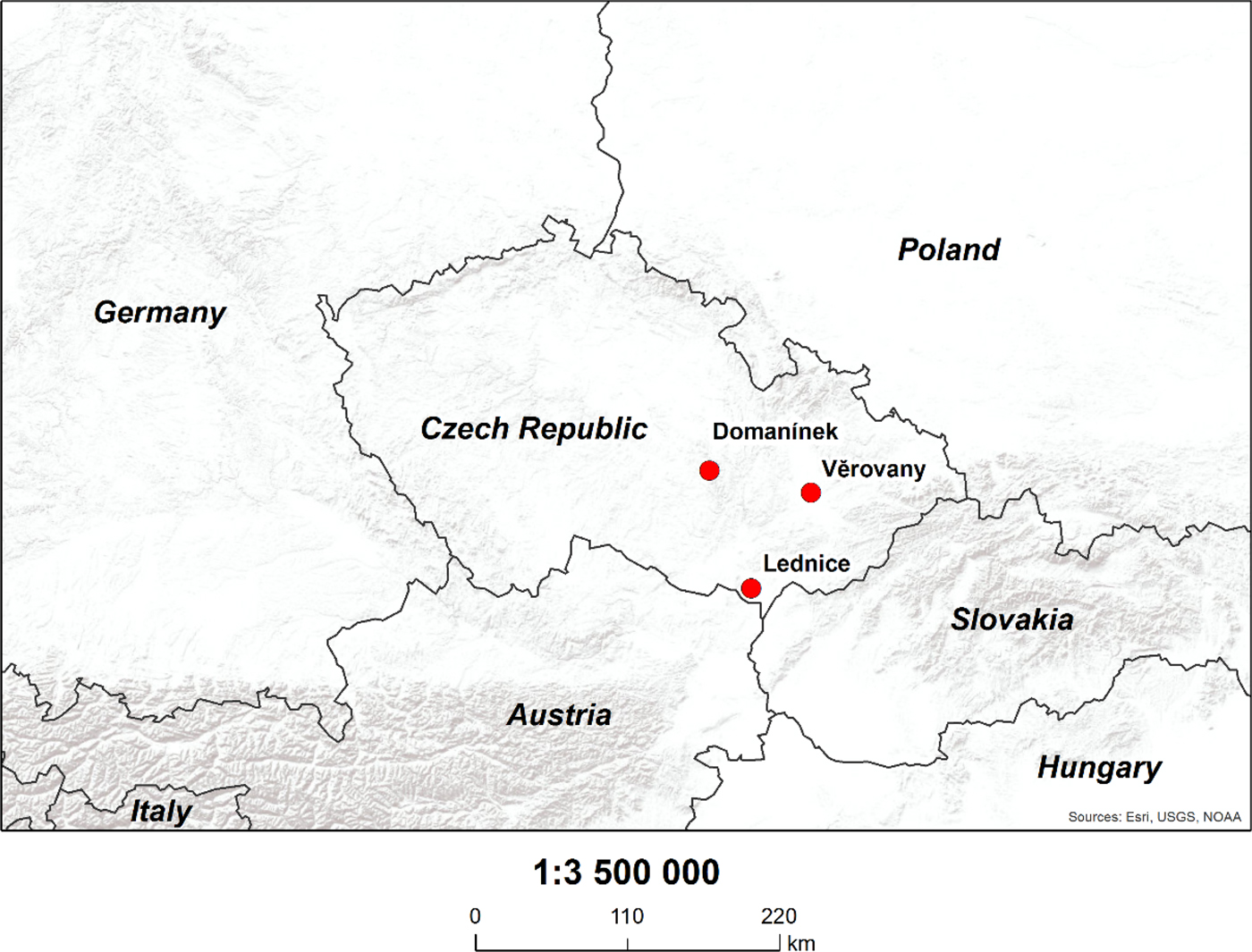
Fig. 1. Map of the Czech Republic indicating the study locations.
The Czech Republic comprises various soil types and climatic conditions. The selected locations represent three basic regimes. Lednice is a warm and relatively dry spring barley growing region. Věrovany is located in the most fertile area of the country, with warm temperatures and generally sufficient rainfall conditions, and Domanínek represents the coolest and wettest of all three sites. The main characteristics of each location are summarized in Table 1.
Table 1. Basic characteristics of the study locations. The climate data are derived from the years 1971–2000 (Tomiška et al. Reference Tomiška, Sládková and Vaňková2003; Tolasz Reference Tolasz2007; Hájková & Dahl Reference Hájková and Dahl2012)

The first step included the calibration and subsequent validation of a crop model ensemble. Within the calibration, parameters for length of the vegetative and reproductive development stages were modified manually using sensitivity analysis. Calibration and validation were performed using experimental data from the Central Institute for Supervising and Testing in Agriculture (SIAST) multi-year field experiments in the selected locations. These data were combined with data from a 4-year field experiment for the spring barley variety ‘Tolar’ in 2011 and 2012 and a variety with the same properties, ‘Bojos’, in 2013 and 2014 in Domanínek (Table 2). The lengths of the growing season and the flowering stage (growth stage [GS] 61, Zadoks et al. Reference Zadoks, Chang and Konzak1974), time to maturity (GS 90) and grain yields were recorded for all years and all study locations. Above-ground biomass yields were not available (Fig. 2).
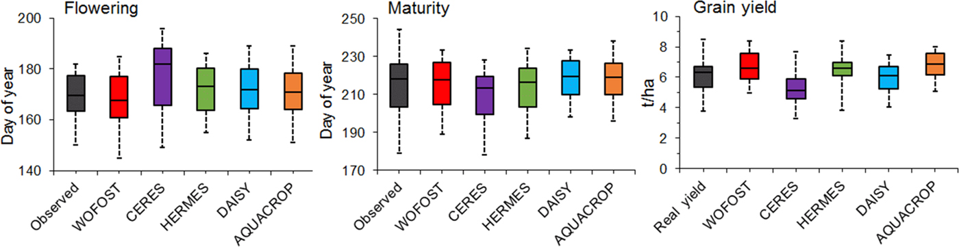
Fig. 2. A comparison of the observed and simulated onset of phenological phases and grain yields for the study locations and the years referenced in Table 1. Boxplots delimit the inter-quartile range (25–75 percentiles) and show the minimum value, maximum value and median.
Table 2. Overview of years and study locations from which simulation outputs of crop models were used
Measurements
In the second step, the ET (Figs 3 and 4), Ta (Figs 3 and 4) and soil water balance (SWB) (Figs 5 and 6) were compared based on model outputs. Simulated values of ETa, reference ET (ETo) and SWB were compared with measured values (ETa, ETo, SWB) for Domanínek from 2011 to 2014 (Figs 4 and 5). The data, which were used as reference data for ET (ETa, ETo), were measured from data by two meteorological stations permanently located on turfgrass at Domanínek (49°31′28″N, 16°14′30″E and 540 m asl; 49°31′18″N, 16°14′10″E and 575 m asl). The actual evapotranspiration of the turfgrass was measured using the Bowen ratio energy balance method. Measurements and data processing have been extensively described in a previous study by Fischer et al. (Reference Fischer, Trnka, Kučera, Deckmyn, Orság, Sedlák, Žalud and Ceulemans2013). Temperature and humidity gradients were measured by combined EMS 33 instruments placed in AL 070/1 radiation shields (EMS Brno, Czech Republic). The net radiation was measured by an NR 8110 net radiometer (Philipp Schenk GmbH Wien, Austria), and the soil heat flux was monitored by an HFP01 sensor (Hukseflux Thermal Sensors, Netherlands). Measurements were taken every minute and logged as half-hour averages. Raw data of latent heat flux were subjected to quality control filtering according to Guo et al. (Reference Guo, Zhang, Kang, Du, Li and Zhu2007). Gaps in the flux data were filled using the algorithm of Reichstein et al. (Reference Reichstein, Falge, Baldocchi, Papale, Aubinet, Berbigier, Bernhofer, Buchmann, Gilmanov, Granier, Grünwald, Havránková, Ilvesniemi, Janous, Knoh, Laurila, Lohila, Loustau, Matteucci, Meyers, Miglietta, Ourcival, Pumpanen, Rambal, Rotenberg, Sanz, Tenhunen, Seufert, Vaccari, Vesala, Yakir and Valentini2005), as implemented in the R package REddyProc (http://r-forge.r-project.org/projects/reddyproc/). The soil water balance was measured using the time domain reflectometry (TDR) method, (CS 616, Campbell Scientific Inc., Shepshed, UK): TDR sensors were placed vertically to monitor the SWB from the surface to a depth of 0.3 m in field experiments with spring barley in Domanínek at the central time during the growing seasons from 2011 to 2014 (Fig. 5).

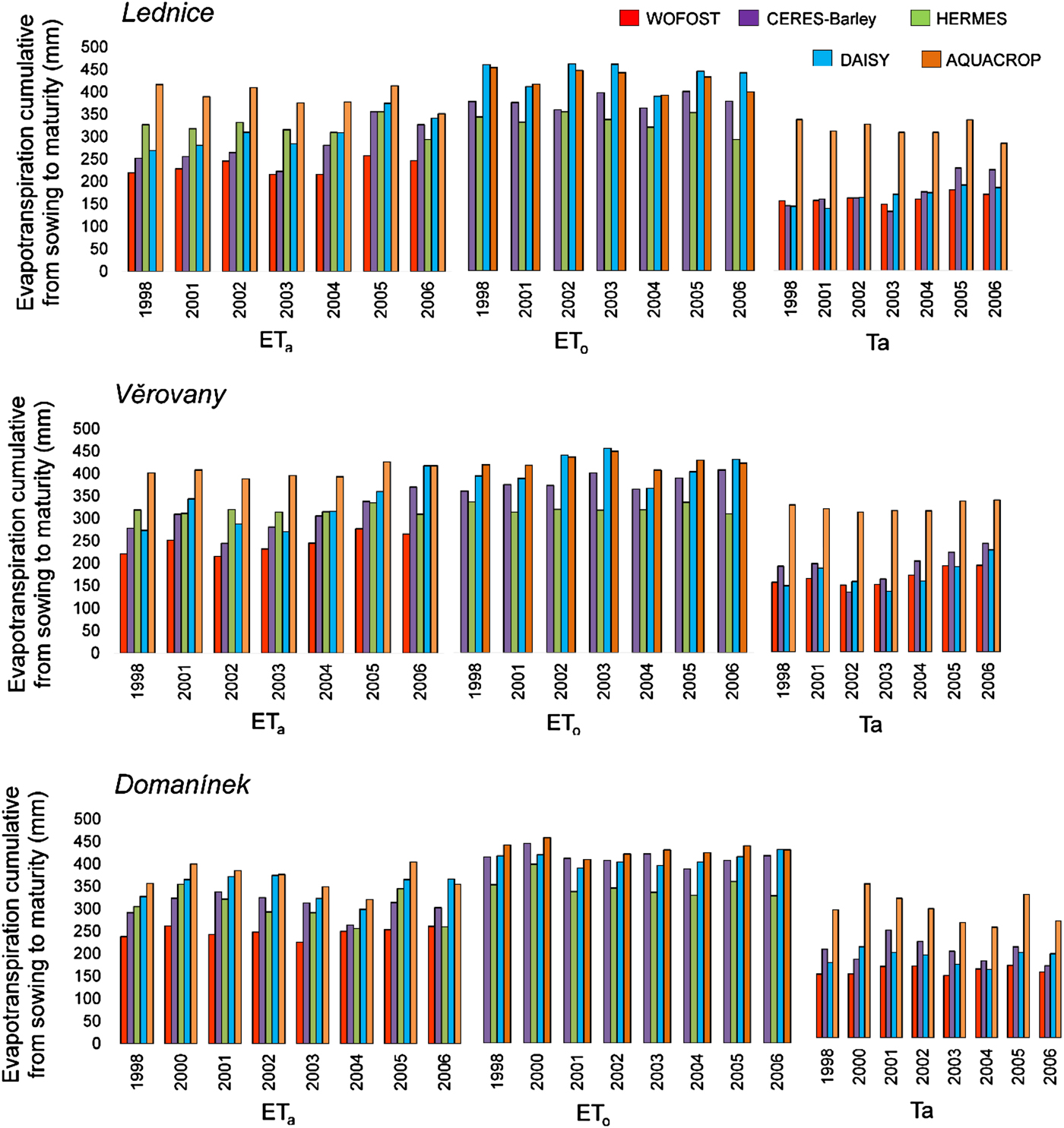
Fig. 3. Simulated components of evapotranspiration (ETa = actual evapotranspiration, ETo = reference evapotranspiration, Ta = actual transpiration) by five crop models, accumulated from sowing to maturity, at three locations during the years given in X-axis.
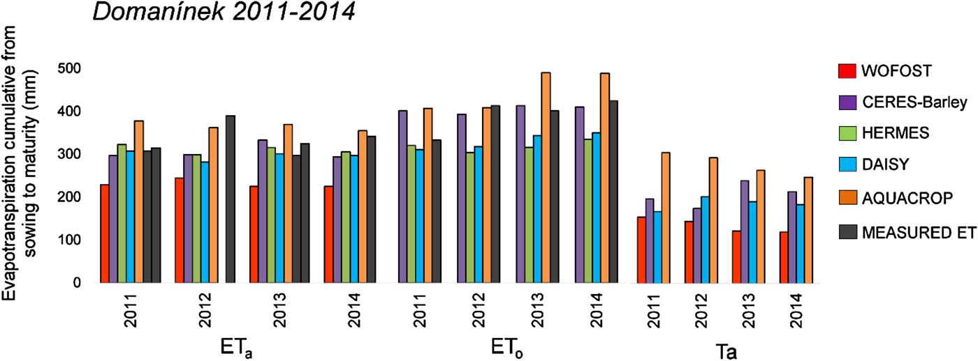
Fig. 4. Simulated and measured components of evapotranspiration (ETa = actual evapotranspiration, ETo = reference evapotranspiration, Ta = actual transpiration) for the study location Domanínek from 2011 to 2014. Measured ETo was obtained from data of one meteorological station and measured ETa from data of both stations. For 2012 and 2014, relevant seasonal data for both meteorological stations are not available. Therefore, measurement were performed for only one of the stations. The measured ETa and ETo values for the turfgrass were used as reference data.
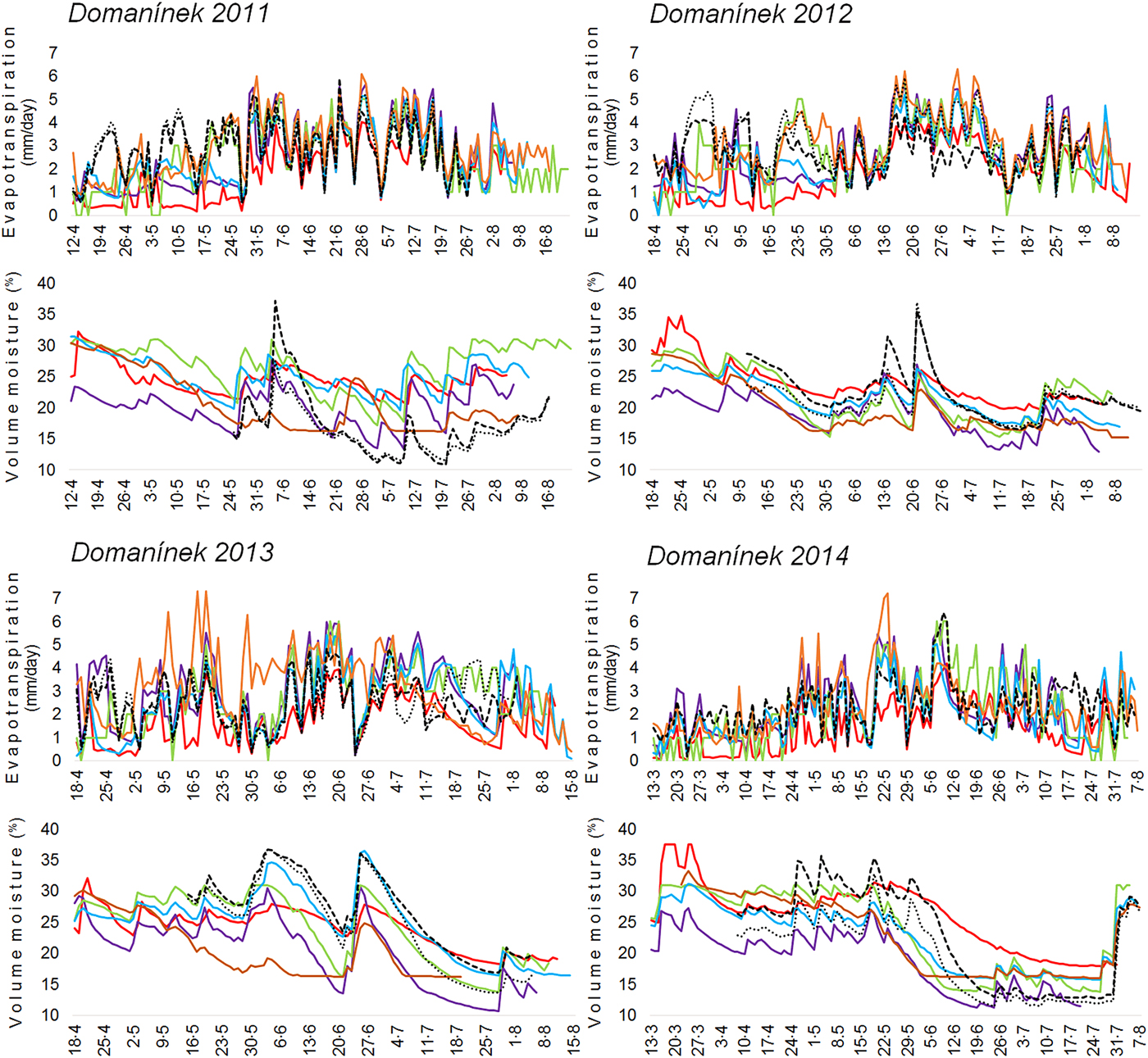
Fig. 5. Comparison between the simulated and measured actual evapotranspiration (ETa) and soil water balance (SWB) for spring barley from soil layer 0–0.3 m between sowing and maturity at the study location Domanínek from 2011–2014. Values measured ETa were obtained from data of two meteorological stations. For 2012 and 2014, relevant seasonal data for both meteorological stations are not available. Therefore, measurements were performed for only one of the stations.

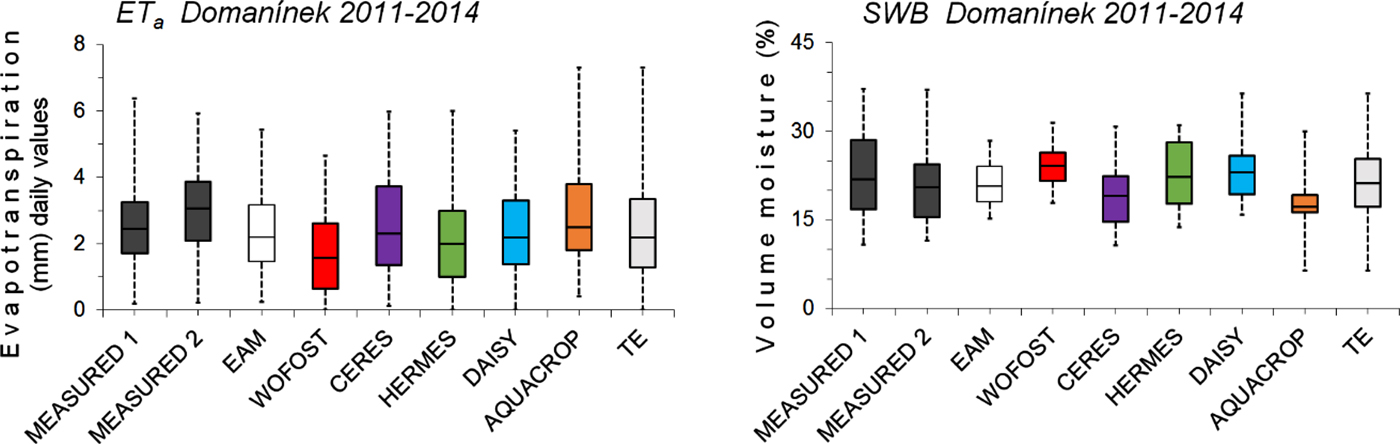
Fig. 6. Comparison between the simulated and measured actual evapotranspiration (ETa) and soil water balance (SWB) for spring barley for the study location Domanínek from 2011 to 2014. Boxplots delimit the inter-quartile range (25–75 percentiles) and show the minimum value, maximum value and median. EAM is ensemble arithmetic mean, TE is total ensemble.
Crop models and methods for calculating evapotranspiration and soil water balance
The current paper describes various results from the selected models. The models and approaches for the calculations used in the current study are described as follows (Table 3).
Table 3. Modelling approaches regarding the main processes determining crop growth and development

(a) Crop phenology as a function of: T = temperature, DL = photoperiod (daylength), (b) Yield formation depending on: B = above-ground biomass, Gn = number of grains, HI = harvest index, PRT = partitioning during reproductive stages, (c) Approaches for calculating evapotranspiration: P = Penman approach, PM = Penman–Monteith approach, PT = Priestley–Taylor approach, (d) Water dynamics approach: C = capacity approach, R = Richards approach, (e) Leaf area development and light interception: D = detailed approach (e.g. layers of canopy), S = simple approach (e.g. LAI), (f) Light utilization: RUE = radiation use efficiency approach, P-R = gross photosynthesis–respiration), TE = transpiration efficiency biomass growth.
Approaches for calculating evapotranspiration
Approaches to ET calculations (Table 3) vary from quite simple (empirical or semi-empirical) requiring only information on monthly average temperatures, to complex (more physical), requiring daily data on maximum and minimum temperature, solar radiation, humidity and wind speed, as well as characteristics of the vegetation (Eitzinger et al. Reference Eitzinger, Marinkovic and Hosch2002; Fischer Reference Fischer2012). The model computes daily net solar radiation. Evapotranspiration (combination of soil evaporation and plant Ta) can be limited by low solar radiation and cool temperatures (low leaf area index, low soil water content, low root length density and their distributions relative to each other) (detailed in Ritchie Reference Ritchie1972).
WOFOST (WOrld FOod STudies), as one of the selected models, uses the Penman (P) approach (Penman Reference Penman1956), adapted according to Frère & Popov (Reference Frére and Popov1979), to calculate ET. In WOFOST, the actual crop Ta is determined by the potential ET time correction factors for the degree of light interception, the degree of water stress and the crop in general (Wolf & De Wit Reference Wolf and De Wit2003). Weather data must include wind and humidity data (Doorenbos & Pruitt Reference Doorenbos and Pruitt1977). The P approach is elucidated by the following equation:
 $$ET = \displaystyle{{\Delta R_{{\rm n},{\rm a}} + {\rm \gamma E}_{\rm a}} \over {\matrix{ {\Delta} \, + \cr} {\rm \gamma}}} $$
where ET is the evapotranspiration rate, R(n,a) is the net absorbed radiation (expressed in equivalent evaporation), Ea is the evaporative demand, Δ is the slope of the saturation vapour pressure curve and γ is a psychometric constant (Supit et al. Reference Supit, Hooijer and Van Diepen1994).
CERES-Barley calculates ET based on the Priestley–Taylor (PT) approach in the current study. The PT equation is useful for the calculation of daily ET in case when weather inputs for the aerodynamic term (relative humidity, wind speed) are unavailable. This radiation-based method approach requires only daily solar radiation and temperature (Ritchie Reference Ritchie1972). The equation is given as:
 $${\rm \lambda} ET = \alpha \displaystyle{{S\;} \over {S + {\rm \gamma}}} (R_{\rm n} - G)$$
where ET is evapotranspiration, λ is the latent heat of vaporization, α is a model coefficient (which Priestley and Taylor allowed to vary for drying conditions), S is the slope of the saturation vapour density curve, γ is a psychrometric constant, Rn is the net radiation, and G is the soil heat flux (Priestly & Taylor Reference Priestly and Taylor1972; Flint & Childs Reference Flint and Childs1991; Ngongondo et al. Reference Ngongondo, Xu, Tallaksen and Alemaw2013).
The approach of Penman–Monteith (PM) is used to calculate ET for the remainder of the selected models: HERMES, DAISY and AQUACROP. Unlike the original P model, in the PM model, the mass-transfer evaporation rate is calculated based on physical principles (Ponce Reference Ponce1989). The ‘full-form’ PM equation can be expressed as follows:
 $$ET = \displaystyle{{\Delta (R_{\rm n} - {\rm G}) + {\rm \; \rho} _{\rm a} {\rm c}_{{\rm p}\;} \; (e_{\rm s} - e_{\rm a} )/r_{\rm a}} \over {(\Delta + {\rm y}\; (1 + (r_{\rm s} /r_{\rm a} )))\rho _{\rm w} {\rm \lambda}}} $$
where ET is the evapotranspirative flux expressed as depth per unit time, Δ is the slope of the saturation vapour pressure v. temperature curve, Rn is the net radiation flux density at the surface, G is the sensible heat flux density from the surface to the soil (positive if the soil is warming), ρa is the air density, cp is the specific heat of moist air at a constant pressure, es is the saturation vapour pressure at air temperature, ea is the actual vapour pressure of the air, ra is the aerodynamic resistance to turbulent heat or vapour transfer from the surface to some height z above the surface, y is a pyschrometric constant, r s is the bulk surface resistance describing the resistance to flow of water vapour from inside the leaf, vegetation canopy or soil to outside the surface, ρ w is the density of water, and λ is the latent heat of vaporization (Allen et al. Reference Allen, Pruitt, Wright, Howell, Ventura, Snyder, Itenfisu, Steduto, Berengena, Yrisarry, Smith, Pereira, Raes, Perrier, Alves, Walter and Elliott2006).
Depending on approaches for calculating ET, crop models require different meteorological data (Palosuo et al. Reference Palosuo, Kersebaum, Angulo, Hlavinka, Moriondo, Olesen, Patil, Ruget, Rumbaurc, Takáč, Trnka, Bindi, Çaldağ, Ewert, Ferrise, Mirschel, Şaylan, Šiška and Rötter2011).
Approaches for calculating soil water balance
Soil water balance is one of the most important parts of the models. According to the models, the soil profile is divided into root zone layers with different water supplies. Each layer has an associated horizon, defining the unique physical properties of that layer (Abrahamsen & Hansen Reference Abrahamsen and Hansen2000). Accordingly, the incoming and outgoing water flows are simulated. WOFOST, CERES-Barley, HERMES and AQUACROP calculate the water balance using the capacity approach (Table 3). This works on the basis of estimated water consumption by ETa, which depends on the course of the meteorological elements, soil moisture availability and characteristics of the vegetation cover or surface (Boogaard et al. Reference Boogaard, van Diepen, Rötter, Cabrera and van Laar1998).
WOFOST has the simplest approach for calculating soil water balance among the selected models. The model considers three soil layers: the rooted zone between the soil surface and the actual rooting depth, the lower zone between the actual rooting depth and the maximum rooting depth, and the sub-soil below the maximum rooting depth. The available soil water contained in the rooted zone, which is directly at the disposal of the crop, is defined as the product of the rooting depth and the current available soil water content (van Diepen et al. Reference van Diepen, Rappoldt, Wolf and Van Keulen1988; Eitzinger et al. Reference Eitzinger, Trnka, Hösch, Žalud and Dubrovský2004). WOFOST does not consider the possible influence of groundwater or its potential capillary rise and treats the soil as a homogeneous layer (Supit et al. Reference Supit, Hooijer and Van Diepen1994; Eitzinger et al. Reference Eitzinger, Trnka, Hösch, Žalud and Dubrovský2004).
The most comprehensive approach among the selected models is that of DAISY, which calculates the water balance between the surface and the soil. DAISY determines the movement of water in soil using a numerical solution of Richards’ equation (Abrahamsen & Hansen Reference Abrahamsen and Hansen2000; van Dam & Feddes Reference van Dam and Feddes2000), which can simulate the water balance at the desired depth (Richards Reference Richards1931). DAISY simulates the movement of water in the soil based on potential theory. The ability of a soil to supply water is determined by the simulated potential infiltration rate, which is based on conditions in the soil. Transpiration is determined by the water intake of roots, depending on the depth of rooting and root density.
More details about model construction and functioning can be found in the literature, e.g. Jones & Kiniry (Reference Jones and Kiniry1986); van Diepen et al. (Reference van Diepen, Rappoldt, Wolf and Van Keulen1988); Kersebaum (Reference Kersebaum1995); Ritchie et al. (Reference Ritchie, Singh, Godwin, Bowen, Tsuji, Hoogenboom and Thornton1998); Tsuji et al. (Reference Tsuji, Hogenboom and Thorton1998) or Hsiao et al. (Reference Hsiao, Heng, Steduto, Rojas-Lara, Raes and Fereres2009).
A comparative analysis was used to compare the simulations ETa and SWB for Domanínek 2011–2014. Simulation results of crop models were subjected to statistical analysis by means of descriptive statistical indices and statistical parameters such as maximum, minimum and mean value; standard deviation; coefficient of variation and variance; root mean square error (RMSE), which describes the average absolute deviation between the observed and modelled values; the mean bias error (MBE) as an indicator of the average systematic error (Davies & McKay Reference Davies and McKay1989) and index of agreement (IA), developed by Willmott (Reference Willmott1981), was used as a more general indicator of modelling efficiency (Table 4). MBE, RMSE and IA can be calculated as follows:
 $$\eqalign{&{\rm MBE} = \displaystyle{{\mathop \sum \nolimits_{i = 1}^n (S_i - O_i )} \over n}\quad {\rm RMSE} = \sqrt {\displaystyle{{\mathop \sum \nolimits_{i = 1}^n (O_i - S_i )^2} \over n}} \cr & \quad {\rm IA} = 1 - \displaystyle{{\mathop \sum \nolimits_{i = 1}^n (S_i - O_i )^2} \over {\mathop \sum \nolimits_{i = 1}^n ( \vert \dot S \vert + \vert \dot O \vert )^2}}}$$
where S i is the simulated value of the variable, O i is the measured value of the variable, n is the number of pairs of observed and estimated values,  ${\bar{\rm S}}$ is the average simulated value of the variable,
  ${\bar{\rm O}}$ is the average measured value of the variable and
  ${\dot{\rm S}}$ = │S i − (S i −
  ${\bar{\rm S}}$)│ and
  ${\dot{\rm O}}$ = │O i − (O i −
  $\overline {{\rm O})} $│.
Table 4. Descriptive statistics calculated for the ETa and SWB and results of models comparison with the measured values for Domanínek 2011–2014
EAM, ensemble arithmetic mean; Min, minimum; Max, maximum; Av, mean value; SD, standard deviation; Var, variance; CV, coefficient of variation.
Calculation of water use efficiency
Water use efficiency can be defined and calculated in a variety of different ways (Blum Reference Blum2009; Medrano et al. Reference Medrano, Tomas, Martorell, Flexas, Hernández, Rosseló, Pou, Escalona and Bota2015; Cammarano et al. Reference Cammarano, Rötter, Asseng, Ewert, Wallach, Martre, Hatfield, Jones, Rosenzweig, Ruane, Boote, Thorburn, Kersebaum, Aggarwal, Angulo, Basso, Bertuzzi, Biernath and Wolf2016). In the current work, calculation and comparison of WUE used simulated outputs of Ta, ETa, dry matter of above-ground biomass and grain yield of spring barley. An equation for calculating WUE was determined as follows:
 $$\eqalign{ & WUE\; ({\rm kgDM/m}^{\rm 3} {\rm H}_{\rm 2} {\rm O}) \cr & = \displaystyle{{\; Dry\; weight\; of\; yield\; ({\rm kg/ha})} \over {\matrix{ {Crop\; water\; supply\; ({\rm m}^{\rm 3} {\rm \; H}_{\rm 2} {\rm O/ha}) = ETa\; or\; Ta\;} \cr}}}} $$
Water use efficiency is represented in units of kg/m3, where crop production is measured in kg/ha and water use is estimated as mm of water applied or received as rainfall, converted to m3/ha (1 mm = 10 m3/ha) (Drechsel et al. Reference Drechsel, Heffer, Magen, Mikkelsen and Wichelns2015).
The combination of two separate processes whereby water is lost from the soil surface by evaporation and from the crop by Ta is referred to as ET (Allen et al. Reference Allen, Pereira, Raes and Smith1998). In a purely hydrological context, WUE has been defined as the ratio of the volume of water used productively (Stanhill Reference Stanhill1986). Above-ground biomass accumulation, and consequently grain yield, has been shown to be inextricably linked to Ta (Sinclair et al. Reference Sinclair, Tanner and Bennett1984). Water use efficiency should therefore be calculated from Ta. However, evaporation is the main factor affecting the total amount of water consumed during the growing season. In the current study, WUE has been calculated using both Ta (WUETa, Fig. 7) and ETa (WUEETa, Fig. 8).

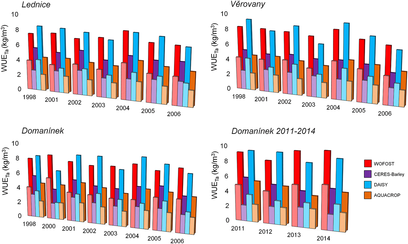
Fig. 7. Comparison of water use efficiency (WUE) values calculated from simulated transpiration (Ta) and grain yield (lower column) and above-ground biomass (higher column) with colours as given in list of models, by four crop models at three study locations for 1998 and 2001–2006 at Lednice and Věrovany and for 1998 and 2000–2006 at Domanínek, and additional at Domanínek during 2011–2014.

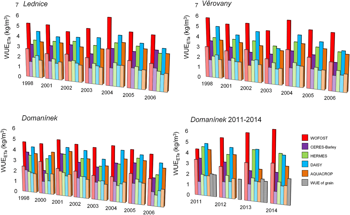
Fig. 8. Comparison of water use efficiency (WUE) values calculated from simulated and measured actual evapotranspiration (ETa) and grain yield (lower column) and above-ground biomass yield (higher column) with colours as given in list of models, by five crop models at three study locations for 1998 and 2001–2006 at Lednice and Věrovany and for 1998 and 2000–2006 at Domanínek, and additional at Domanínek during 2011–2014. WUE of grain was calculated from the measured values. Graph ‘Domanínek 2011–2014’ show calculated results WUEEta from measured ETa. Values measured ETa were obtained from data of two meteorological stations. For 2012 and 2014, relevant seasonal data for both meteorological stations are not available. Therefore, measurements were performed for only one of the stations.
The percent deviation (D i) between measured and simulated ETa and calculated WUEETa was determined as follows (Table 5) (Bitri & Grazhdani Reference Bitri and Grazhdani2015):
 $$D_i = (simulated\; value - measured\; value)\; \times \; \displaystyle{{100} \over {measured\; value}}$$
Table 5. Comparison between measured and simulated seasonal sums of actual evapotranspiration (ETa) and water use efficiency (WUEETa) for the study location Domanínek from 2011 to 2014. Measured ETa was obtained from data of two meteorological stations. For 2012 and 2014, relevant seasonal data for both meteorological stations are not available. Therefore, comparison was performed for only one of the stations in these years
EAM, ensemble arithmetic mean; D i, deviation, sums of ETa (mm), WUEETa (kg/m3).
The arithmetic mean of the crop models simulations as EAM and the total range of crop models simulations as TE was shown by the use of boxplots (Figs 6, 9 and 10).
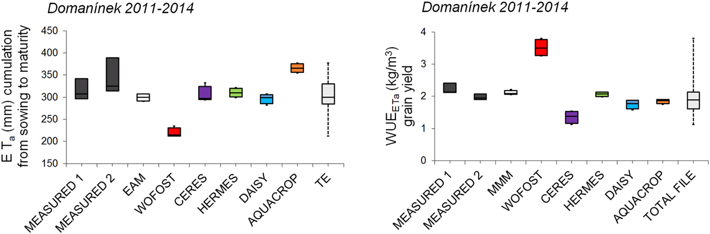
Fig. 9. Comparison of the seasonal sums of ETa and water use efficiency (WUEETa) for grain yield of spring barley, calculated from simulated and measured ETa values for selected crop models at the study location Domanínek from 2011 to 2014. Boxplots delimit the inter-quartile range (25–75 percentiles) and show the minimum value, maximum value and median. EAM is ensemble arithmetic mean, TE is total ensemble.

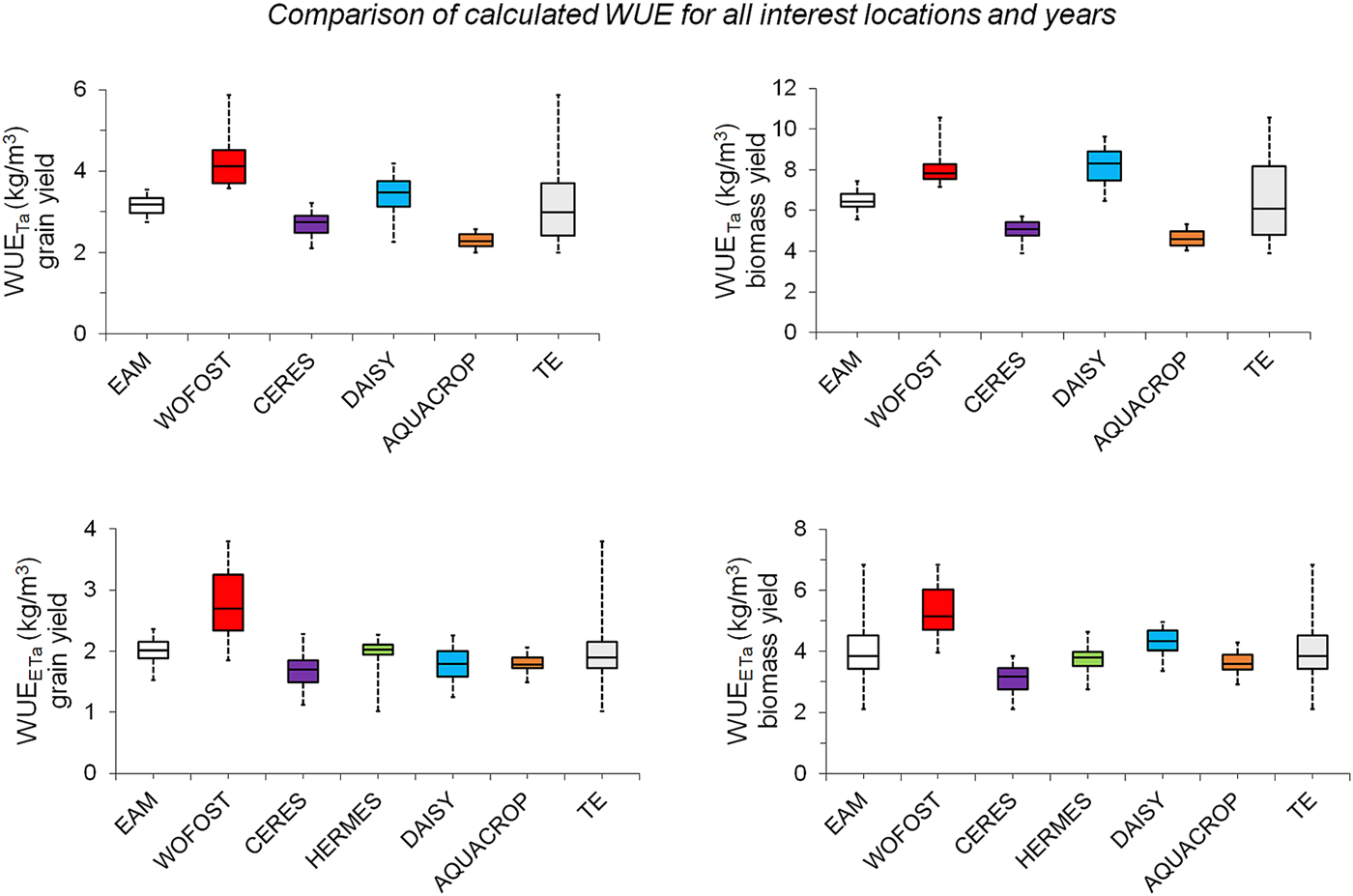
Fig. 10. Comprehensive comparison of calculated WUETa values and WUEETa values for the study locations: Lednice for 1998 and 2001–2006, Věrovany for 1998 and 2001–2006, Domanínek for 1998, 2000–2006 and 2011–2014. Boxplots delimit the inter-quartile range (25–75 percentiles) and show the minimum value, maximum value and median. EAM is ensemble arithmetic mean, TE is total ensemble.
Results
Flowering, maturity and grain yield
The crop models were calibrated and validated based on approximations of the observed phenological phases (flowering and maturity) and grain yields, to produce simulated phenological phases and grain yields (Fig. 2).
The simulation results for spring barley with respect to the phenological phase of flowering (GS 61) in the Czech Republic showed a slight deviation from the observations, from −1 to +9 days. CERES-Barley simulated later flowering dates than the other models. Phenological phase maturity (GS 90) was less variable among the models, with differences of −7 to +5.5 days as compared with the observations. These results indicate that the simulated length of the growing season is different for each individual model. The simulation results for grain yield showed deviations from the real grain yield ranging from −1 to +1.28 t/ha. Detailed calibration and validation results can be found in the Supplementary Material.
Evapotranspiration and soil water balance
Evapotranspiration was calculated for all study years and study locations (Tables 1 and 2) by the different approaches incorporated within the selected crop models (Table 3). The obtained values of cumulative ET can be found in Figs 3 and 4.
In the current study, the sum of ETa during the growing seasons ranged from 201.5 to 426.2 mm among the applied approaches, while ETo ranged from 226.9 to 490 mm. The deviation of ETa from ETo is evident. The crop matures and the canopy cover declines during the growing season, therefore, the ETa is lower. Crop models using the PM approach to calculate the sum of ET often produced higher values than models with a different approach. With the exception of AQUACROP (PM approach), which simulated the highest values, and WOFOST (P approach), which simulated the lowest values, the results are within a relatively small range. Transpiration, part of ETa, is an important factor for water balance. Different approaches can cause deviations in the results, which are clearly shown in Figs 3 and 4, particularly for AQUACROP.
The success of individual models can be compared on the basis of ETa and SWB reference data from Domanínek 2011–2014 (Figs 4–6, Tables 4 and 5). The results of statistical parameters showed that crop models HERMES (IAETa/SWB 0.84/0.78), DAISY (IAETa/SWB 0.78/0.81) and CERES-Barley (IAETa/SWB 0.78/0.75) showed the closest conformity. The crop model WOFOST (IAETa/SWB 0.62/0.72) showed the poorest conformity. The values of IAETa/SWB for EAM were 0.81/0.73. When compared RMSEETa/SWB and IAETa/SWB as indicators, it was found that several models, such as HERMES, DAISY and CERES-Barley, do almost as well as the EAM (Tables 5 and 6, Figs 6 and 9).
Table 6. An overview of the range of water use efficiency (WUE) values calculated from the outputs of individual models (WUETa/WUEEta)

EAM, ensemble arithmetic mean.
The largest DiETa between measured and simulated values was in 2012. The maximum D i with value −45% was reached by WOFOST (Table 5). The zero D i was achieved in one case in 2011 by DAISY and EAM.
Water use efficiency
The differences in the simulations of seasonal Ta, ETa, length of growing season and yield of individual models resulted in different WUE values for spring barley. The outputs of the HERMES model did not include Ta.
The values of WUETa ranged from 3.9 to 10.5 kg/m3 for above-ground biomass yield and from 2.0 to 5.9 kg/m3 for grain yield (Fig. 7). The values of WUEETa were lower, ranging from 2.1 to 6.8 kg/m3 for above-ground biomass yield and from 1.0 to 3.8 kg/m3 for grain yield (Fig. 8).
Figure 8 also shows the WUEETa values calculated from measurements for use as reference data. These values ranged from 1.9 to 2.4 kg/m3 for grain yield.
The highest WUE values were calculated from outputs of the crop model WOFOST, which simulated the lowest Ta/ET among all selected models. The lowest WUE values were calculated from outputs of the models CERES-Barley and AQUACROP.
For the WUEETa values calculated from simulations and measurements, the best agreements were shown by the HERMES model, with an average D i −0.83%, and AQUACROP, with an average D i 10.50%. The values of WUEETa calculated from simulations of the WOFOST and CERES-Barley models showed the poorest agreement (average D i of 67.33 and −33.16%, respectively; Fig. 9 and Table 5).
Finally, Fig. 10 shows a comparison of the WUE values calculated from simulations of the crop models. The results confirm that the WUE calculated from the outputs of the WOFOST model is overestimated compared with that of other models, often with the largest variation. The values of WUETa calculated from the outputs of CERES-Barley and AQUACROP are nearly the same. The values of WUEETa for CERES-Barley, HERMES, DAISY and AQUACROP also show strong agreement with each other.
Discussion
The results of the first part of the study show that the WOFOST model, using the P approach, simulates low ETa sums compared with the other models, which use the PM approach. Sums of ETa values during the vegetative season were 240 mm, on average, for WOFOST. For models using the PM approach, the sum values of ETa were 340 mm on average. This finding is similar to those reported by Eitzinger et al. (Reference Eitzinger, Marinkovic and Hosch2002), where sums of ETa simulated with WOFOST were low, at 205 mm on average, and the highest sums of ETa, 330 mm on average, were simulated with models using the PM approach, as in the current study. WOFOST was also shown to underestimate ETa compared with other models in a study by Rötter et al. (Reference Rötter, Palosuo, Kersebaum, Angulo, Bindi, Ewert, Ferrise, Hlavinka, Moriondo, Nendel, Olesen, Patil, Ruget, Takáč and Trnka2012), where DAISY, HERMES and CERES-Barley simulated the highest ETa values, with high similarity among the values, as in the current study. AQUACROP simulated the highest Ta of the models. The value of Ta was calculated as 78% of ETa on average. A similar result was reported by Zeleke et al. (Reference Zeleke, Luckett and Cowley2011), in which AQUACROP produced a Ta value of 75% of ETa. The largest DiETa is from 2012 may be due to the fact that the ETa reference value was measured at only one meteorological station. There is no other reference value that would allow for verification of measurement accuracy.
As in the studies of Federer et al. (Reference Federer, Vörösmarty and Fekete1996), Eitzinger et al. (Reference Eitzinger, Marinkovic and Hosch2002) and Rácz et al. (Reference Rácz, Nagy and Dobos2013), the differences between ET calculation approaches (P, PT, PM) in the current study amounted to hundreds of millimetres per growing season. The PM approach had on average the highest match from measured ET. The PT approach performed slightly poorer while the P approach had the highest discrepancy with the reference data, as was also the case in the studies of Xu & Singh (Reference Xu and Singh2002) and Xing et al. (Reference Xing, Chow, Meng, Rees, Stevens and Monteith2008). Weaknesses can be found in P, PT and PM approaches. The P approach was mainly developed for a short crop, such as grass. In semi-arid areas, simulated Ta may also be too low. Further, wind velocity was solved empirically (Penman Reference Penman1948; Wolf & De Witt Reference Wolf and De Wit2003; Subedi & Chávez Reference Subedi and Chávez2015); therefore, the P approach may not work properly under all climatic conditions. The PT approach does not take account of saturation vapour pressure, therefore is useful for mild and humid tropical climates but not very suitable for arid and windy areas (Novák Reference Novák1995; Schneider et al. Reference Schneider, Ketzer, Breuer, Vaché, Bernhofer and Frede2007; Fischer Reference Fischer2012; Rácz et al. Reference Rácz, Nagy and Dobos2013). The PM approach is considered as one of the best methods for ET calculation. It contains all the parameters included in the energy exchange process that can be used globally without the need for special modifications. However, the PM approach has the greatest data demands (Allen et al. Reference Allen, Pereira, Raes and Smith1998; Ngongondo et al. Reference Ngongondo, Xu, Tallaksen and Alemaw2013; Remesan & Holman Reference Remesan and Holman2015).
The accuracy of a given approach depends on the climatic and soil conditions (SWB) of the study location (Nash Reference Nash1989; Rácz et al. Reference Rácz, Nagy and Dobos2013) and model parameterization. The variability among simulations of crop models in ET and SWB indicates that there are differences in the way the processes that affect water use are modelled. Crop models use either a simpler capacity approach or a more detailed Richards approach. Simulated SWB is not dependent only on model approaches for calculating water balance. For example, individual crop models, which have different approaches to simulating soil water extraction by roots (e.g. the maximum rooting depth is important) deal also with the soil profile at different degrees of resolution (De Wit & Van Keulen Reference De Wit and Van Keulen1987; Wu & Kersebaum Reference Wu, Kersebaum, Ahuja, Reddy, Saseendran and Yu2008; Palosuo et al. Reference Palosuo, Kersebaum, Angulo, Hlavinka, Moriondo, Olesen, Patil, Ruget, Rumbaurc, Takáč, Trnka, Bindi, Çaldağ, Ewert, Ferrise, Mirschel, Şaylan, Šiška and Rötter2011; Cammarano et al. Reference Cammarano, Rötter, Asseng, Ewert, Wallach, Martre, Hatfield, Jones, Rosenzweig, Ruane, Boote, Thorburn, Kersebaum, Aggarwal, Angulo, Basso, Bertuzzi, Biernath and Wolf2016). The same methods of calculation can produce different results, caused by different parameterizations in the various models (Eitzinger et al. Reference Eitzinger, Marinkovic and Hosch2002). The total range of crop model simulations shows the range and variability of simulations.
Similar results are described with other studies such as Eitzinger et al. (Reference Eitzinger, Trnka, Hösch, Žalud and Dubrovský2004); Hlavinka et al. (Reference Hlavinka, Trnka, Eitzinger, Smutny, Thaler, Žalud, Rischbeck and Křen2010); Andarzian et al. (Reference Andarzian, Bannayan, Steduto, Mazraeh, Barati, Barati and Rahnama2011); Palosuo et al. (Reference Palosuo, Kersebaum, Angulo, Hlavinka, Moriondo, Olesen, Patil, Ruget, Rumbaurc, Takáč, Trnka, Bindi, Çaldağ, Ewert, Ferrise, Mirschel, Şaylan, Šiška and Rötter2011); Abrha et al. (Reference Abrha, Delbecque, Raes, Tsegay, Todorovic, Heng, Vanutrecht, Geerts, Garcia-Vila and Deckers2012); Rötter et al. (Reference Rötter, Palosuo, Kersebaum, Angulo, Bindi, Ewert, Ferrise, Hlavinka, Moriondo, Nendel, Olesen, Patil, Ruget, Takáč and Trnka2012) or Wang et al. (Reference Wang, Wang, Fan and Fu2013). The aforementioned studies dealt with crop models and SWB modelling: values for the statistical parameter IASWB were in the range 0.59 (WOFOST) to 0.93 (CERES-Barley) and for RMSESWB (%) were in the range 0.70 (CERES-Barley) to 13.05 (AQUACROP). In the current study, the statistical parameter IASWB was in the range 0.72 (WOFOST) to 0.81 (DAISY) and RMSESWB (%) was in the range 4.69 (DAISY) to 8.28 (AQUACROP), corresponding with the range of the results for the aforementioned studies.
WOFOST was most distant to SWB measurements and closest to the measured values were DAISY and HERMES, as well as in the study by Rötter et al. (Reference Rötter, Palosuo, Kersebaum, Angulo, Bindi, Ewert, Ferrise, Hlavinka, Moriondo, Nendel, Olesen, Patil, Ruget, Takáč and Trnka2012). Otherwise, it was in the study of Palosuo et al. (Reference Palosuo, Kersebaum, Angulo, Hlavinka, Moriondo, Olesen, Patil, Ruget, Rumbaurc, Takáč, Trnka, Bindi, Çaldağ, Ewert, Ferrise, Mirschel, Şaylan, Šiška and Rötter2011) where measured values were the closest to the WOFOST and HERMES simulations, while CERES and DAISY simulated SWB overstated.
Some of the deviation within the SWB measurements could be connected with the TDR sensors, which have shortcomings (e.g. lower measured soil volume, limited use in soil with a high salinity content and in soils with high electrical conductivity, sensitivity to soil cracks or air pockets) (Hlavinka et al. Reference Hlavinka, Trnka, Eitzinger, Smutny, Thaler, Žalud, Rischbeck and Křen2010; Litschmann Reference Litschmann2010).
The last part of the study concerns WUE. The values of WUE have ranged from 0.7 to 2.8 kg/m3 in studies on spring barley: for example, Katerji et al. (Reference Katerji, Mastrorilli and Rana2008) reported variability in WUE, with values for barley ranging from 1.5 to 2.8 kg/m3. Cossani et al. (Reference Cossani, Slafer and Savin2012) reported lower WUE values for grain and biomass, ranging from 0.7 to 2.3 kg/m3. Cantero-Martinez et al. (Reference Cantero-Martinez, Angas and Lampurlanés2003) found average WUE values for grain and biomass of 2.3 kg/m3 and 1.0 to 1.5 kg/m3, respectively, and Siddique et al. (Reference Siddique, Tennant, Perry and Belford1990) measured WUE at a value of 1.6 kg/m3. In the current study, WUE reference values in the range 1.9–2.4 kg/m3 were calculated for spring barley and grain yield. These values correspond to a narrower range of results than the aforementioned studies.
The values of WUE for spring barley, as calculated from simulations, ranged from 2.1 to 10.5 kg/m3 for above-ground biomass yield and 1.0–5.9 kg/m3 for grain yield.
The values of WUE were calculated in two ways, therefore, the resulting values show greater deviation. The values of WUE based on ETa were more accurate. The reference values were closest to the WUE values obtained from the simulation models HERMES, AQUACROP and DAISY, followed by and CERES-Barley, with the poorest agreement for WOFOST. Average WUEETa values of EAM would be with D i 1.6% included after HERMES.
Table 7 shows WUE values from world studies with an average WUE value of 1.6 kg/m3 for spring barley. This value is slightly lower than the reference WUE value calculated for the study location Domanínek, with an average of 2.1 kg/m3. This discrepancy can be explained by the fact that the other studies on WUE were often performed in semi-arid areas.
Table 7. Overview of the range of water use efficiency (WUE) values for other important crops

a WUE values were calculated from Ta.
Conclusion
The aims of the current study were to compare values calculated from simulations of selected process-based crop models with observational results. Differences were observed between individual models. Some models predicted values that were closer to recordings than others. No model was clearly superior or more robust in terms of WUE accuracy. If average values are taken into account, EAM proved to be the best predictor. However, EAM reduces variability and the result is simplified. In the predictions of the different scenarios, it is important to know the extreme values and the range of uncertainty between different approaches. The degree of variability of the simulated values increases by incorporating the ‘less successful’ models into an ensemble simulation. Simulations are not constant, due to the variety of environmental conditions. For this purpose, it is good to choose a TE approach, which provides a better estimation of the uncertainty of simulation outputs. To lower the level of the degree of uncertainty further research is needed, especially for model inter-comparisons and site-specific model evaluation.
Supplementary material
The supplementary material for this article can be found at https://doi.org/10.1017/S0021859618000060.
Acknowledgements
The current study was supported by the National grant agency project ‘System for monitoring and forecast of impacts of agricultural drought’ No. QJ1610072 and by GACR 16-16549S ‘Soil and hydrological drought in the changing climate’. Experimental work was supported by the Ministry of Education, Youth and Sports of CR within the National Sustainability Program (NPU I), grant number LO1415.