Introduction
The growth and development of animals is a complex phenomenon, influenced by various factors, such as feeding, climate conditions, health and genetics. Species of poultry have widely differing sizes and growth rates as a result of natural selection (Buzala and Janicki, Reference Buzala and Janicki2016).
The comprehension of growth is necessary to formulate simulation models able to predict the nutritional demands of birds and determine the effects of feeding and environmental conditions on their performance (Gous et al., Reference Gous, Moran, Stilborn, Bradford and Emmans1999). These models make it possible to improve management strategies for each life stage or genetic type, with focus on improving important growth traits, and thus enhancing performance and reducing feed costs (Grieser et al., Reference Grieser, Marcato, Furlan, Zancanela, Vesco, Batista, Ton and Perine2018).
Non-linear mathematical models are used to describe the growth of animals during their lifetime, relating weight and age. These models allow datasets consisting of series of weights by age to be condensed into a small number of parameters, to facilitate interpretation and understanding of the phenomenon (Oliveira et al., Reference Oliveira, Lôbo and Pereira2000).
Mixed non-linear modelling permits consideration of the heterogeneity among individuals arising from variables not measured through the inclusion of random effects in the model (Hall and Clutter, Reference Hall and Clutter2004). Therefore, by assuming that the live weight measures of each animal follow the same functional form, the method permits variation of individual parameters to consider deviations from the average curve (Lindstrom and Bates, Reference Lindstrom and Bates1990). Mixed non-linear models have been used previously in studies involving quail growth curves (Kizilkaya et al., Reference Kizilkaya, Balcioglu, Yolcu, Karabag and Genc2006; Aggrey, Reference Aggrey2009; Karaman et al., Reference Karaman, Narinc, Firat and Aksoy2013). However, few studies reporting growth rates have applied mixed models to compare meat and laying quail lines.
Therefore, the objective of the current study was to select the non-linear model with mixed effects that best fits the growth curve of meat and laying quails, employing various types of residuals, and to obtain instantaneous, relative and absolute growth rates of these bird lines.
Materials and methods
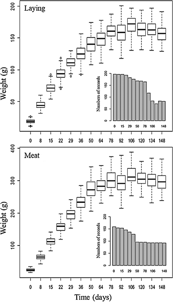
The database used came from Mato Grosso Federal University, Rondonópolis Campus, Brazil, containing weights of female quails bred for meat (Coturnix coturnix coturnix) and laying (Coturnix c. japonica). The weight records referred to 0, 8, 15, 22, 29, 36, 50, 64, 78, 92, 106, 120, 134 and 148 days of age. There was a reduction in the number of records due to the consistency process performed in the database and natural mortality of the birds (Fig. 1). The birds had free access to water and feed and were kept in groups of eight birds in cages with dimensions of 100 cm length × 25 cm width × 20 cm height, equipped with automatic water dispensers and feed troughs.

Fig. 1. Description of the database composed of lines of quail for meat and laying.
The feed consisted mainly of maize meal and soy meal, containing 250 g/kg crude protein (CP) and 2682 kcal metabolizable energy (ME)/kg, from birth to 21 days of age, 230 g/kg CP and 2774 kcal of ME/kg from 22 to 25 days of age, and 219 g/kg CP and 2591 kcal of ME/kg from 26 to 148 days of age, adjusted considering the chemical composition of the feed and nutritional requirements proposed by Albino and Barreto (Reference Albino and Barreto2003).
The mathematical models Brody (Brody, Reference Brody1945), Von Bertalanffy (Von Bertalanffy (Reference Von Bertalanffy1957), Logistic (Nelder, Reference Nelder1961) and Gompertz (Laird, Reference Laird1965) were considered to adjust the growth curves of both lines using non-linear models with mixed effects according to the following equation:
 $$Y_{ij} = f\,(x_{ij},\; \psi _i)\, + \,g\,(x_{ij},\; \psi _i,\epsilon )\,,\; \,1\, \le \,i\, \le \,N,\,1\, \le \,j\, \le \,ni\,,$$
 $$\epsilon _{ij}\,\sim \,N\,(0,\sigma _{\rm e}^2 )\,,$$
 $$\psi _i\, = \,H\,(\mu, c_i,\pi _i).$$
where Y ij is the j-th record of the weight of the i-th bird; N is the number of birds; ni is the number of records of the bird i; f is non-linear growth function; x ij is the matrix of independent variables (j-th recording age and i-th heavy bird); ψ i is the vector of individual parameters; H is a function which describes the covariate model; c i is a vector of known variables; μ is an unknown fixed vector; π i is a random unknown vector; g is the residue function of the model; € is a vector of residual variance; €ij is random residuals with mean zero and variance 1;  $\sigma _{\rm e}^2 $ is the residual variance. Thus, assuming an unknown vector of random normal distribution of size n and where the random residuals are mutually independent, modelling of the residues was performed: constant (g = a and € = a), proportional (g = b f and € = b), combined (g = a + b f and € = a, b) and exponential (t (y) = log (y);Y = feg€).
Growth curve adjustment was performed using a stochastic approximation version of the Expectation Maximization (EM) algorithm for maximum likelihood estimation, the Stochastic Approximation Expectation Maximization (SAEM) algorithm developed by Kühn and Lavielle (Reference Kühn and Lavielle2005) and implemented in the Saemix package (Comets et al., Reference Comets, Lavenu and Lavielle2017) of R version 3.5.1 (2018) (https://www.r-project.org/).
Selection of the best fitting model is related to the explanation of the observed event in a small number of parameters with biological interpretation, i.e. the best model is one that presents a good fit to the observed data with the lowest number of parameters. The Bayesian Information Criterion (BIC) proposed by Schwarz (Reference Schwarz1978) was used to evaluate the quality of fit between observed and predicted data, penalizing the model according to the number of parameters. Therefore, the lowest value for BIC characterizes the model with the highest adjustment quality. The BIC was calculated considering the modification proposed by Kass and Raftery (Reference Kass and Raftery1995) for mixed models, defined as:
 $$BIC\, = \,-\,2\,\log \,l_M\,(y;\hat{\theta} )\, + \,p{\rm log}\,{\rm (}n{\rm )}$$
where  $l_M\,(y;\hat{\theta} )$ represents the likelihood function, considering the approximation method by linearization; n is number of observations; and p is number of parameters adjusted.
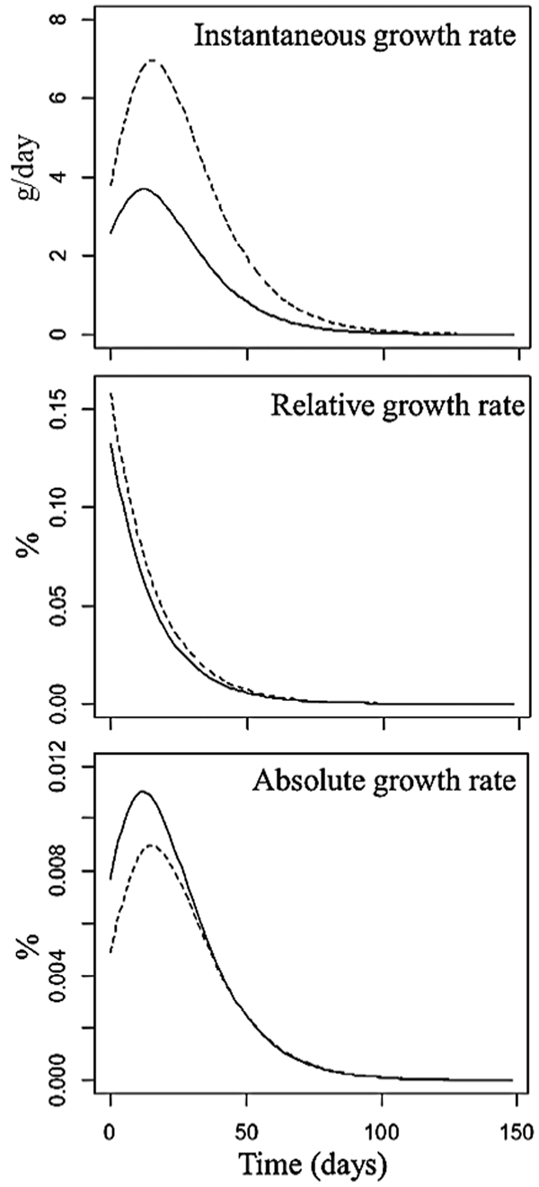
After selecting the model with the best fit, the following were estimated: instantaneous growth rate (IGR), the derivative of Y ij as a function of time (t), representing the increase in weight at each unit of t; absolute growth rate (AGR), the ratio of IGR to asymptotic weight (A), representing the rate of weight gain proportional to the estimated final weight; RIGR, the ratio of IGR in t to the estimated weight (Y) at t, which represents the efficiency of the bird in the conversion of food by body mass; and inflection point (IP), the t when the bird's IGR goes from increasing to decreasing (Table 1).
Table 1. Non-linear models with mixed effects, growth rates and inflection point

A, asymptotic weight (g); B, integration constant; k, average growth rate; t, age (days); e, exponential; IGR, instantaneous growth rate; RIGR, relative growth rate; AGR, absolute growth rate; IP, inflection point; y, equation of the model used; €, error
Results
The Gompertz model, independent of residue type, presented the best fit for the growth curve, followed by the Von Bertalanffy, Logistic and Brody models for the meat line, and the Von Bertalanffy, Brody and Logistic models for the laying line (Table 2). Regarding the types of residue as a function of the model, the combined residue provided the best fit for both strains, except for the Brody (Proportional) model for the meat line.
Table 2. Values of Bayesian Information Criterion (BIC) of mixed non-linear models with different types of residues for quail lines for meat and laying

Applying the selected model (Gompertz with combined residue), it was possible to verify differences in the magnitude of asymptotic weight (A), but it was also noticed that both lines presented values of close to the integration constant (B), average growth rate (k) and IP (Fig. 2). The model showed a good fit to observed data in the initial phase of growth, but less so in the asymptotic phase of the curve of the two lines, over-estimating values for the laying line, but under-estimating and over-estimating for the meat line.

Fig. 2. Observed growth curves (●●●), predicted (˗˗˗˗˗) and inflection point (-----) adjusted by the Gompertz model with combined residue for meat and laying quails lines.
Regarding the estimated parameters, there was a greater amplitude for the A value of the meat line in relation to the laying line (Table 3). For parameter B, the highest amplitude was seen for the laying line, but the same amplitude was verified for k between the lines. There was greater variability for the k parameter in both lines, followed by B and A. Among the lines, there is greater variability in B and k for the meat lines, and A for laying lines. However, estimated variability of the parameters for the studied populations was low (variation coefficient <3.0). The correlation between A and k was significant (P < 0.001) with a value of −0.99 for both lines.
Table 3. Statistics of the parameters estimated by the Gompertz model with combined residue for quail lines for cutting and laying

A, asymptotic weight (g); B, integration constant; k, average growth rate; VC, variation coefficient
The meat line presented higher initial IGR than the laying line (Fig. 3), with a maximum growth rate of 6.95 g/day at 15 days and 3.65 g/day at 11 days of age for the meat and laying lines, respectively, after which both lines began to grow more slowly.

Fig. 3. Instantaneous growth rate (IGR), relative growth rate (RIGR) and absolute growth rate (AGR) for meat (-----) and laying (˗˗˗˗˗˗) quail lines.
The RIGR presented initial values of 0.13% for the meat line and 0.15% for the laying line, reaching minimum values after 50 days of age (Fig. 3). The AGR estimated at birth were 0.004 and 0.007% for the European and Japanese lines, respectively. Thereafter, the AGR steadily increased until the IP (0.008 and 0.01%) and then declined until reaching minimum values near zero at 100 days.
Discussion
Corroborating the results obtained in the current study for the two lines, the Gompertz model has been applied in other studies to fit growth curves for quail (Narinç et al., Reference Narinç, Narinç and Aygün2017; Rossi et al., Reference Rossi, Grieser, Conselvan and Marcato2017). The longitudinal nature of the data, where variance with age is not constant, led to the selection of a heterogeneous residual structure (Craig and Schinckel, Reference Craig and Schinckel2001; Schinckel and Craig, Reference Schinckel and Craig2002).
The estimates of A obtained in the analyses were lower than those described in other studies, which have presented values between 357 and 410 g for meat quail and between 166 and 222 g for laying quail (Mota et al., Reference Mota, Alcântara, Abreu, Costa, Pires, Bonafé, Silva and Pinheiro2015; Firat et al., Reference Firat, Karaman, Başar and Narinc2016; Grieser et al., Reference Grieser, Marcato, Furlan, Zancanela, Vesco, Batista, Ton and Perine2018). However, AGR in the current study was similar to the values reported by the aforementioned authors, near 0.07%. Besides the model used, a possible explanation for the smaller values of A is related to the time period utilized in modelling the curves, since Koncagul and Cadirci (Reference Koncagul and Cadirci2009) found a reduction in the estimate of A with increasing age of birds.
The antagonistic relation found between the parameters A and k also has been described in cattle (Lopes et al., Reference Lopes, Magnabosco, de Souza, de Assis and Brunes2016), buffaloes (Malhado et al., Reference Malhado, Rezende, Malhado, Azevedo, de Souza and Souza Carneiro2017), chickens (Manjula et al., Reference Manjula, Park, Seo, Choi, Jin, Ahn, Heo, Kang and Lee2018) and pigs (Coyne et al., Reference Coyne, Berry, Mäntysaari, Juga and McHugh2015), where the estimates vary between −0.33 and −0.70. Mota et al. (Reference Mota, Alcântara, Abreu, Costa, Pires, Bonafé, Silva and Pinheiro2015) reported correlations of −0.94 and −0.95 for meat and laying quail. This antagonistic association indicates that animals having higher growth rates have lower asymptotic weight or reach their final weight at a younger age (Knižetova et al., Reference Knižetova, Hyanek, Kniže and Prochazkova1991; Lopes et al., Reference Lopes, Magnabosco, de Souza, de Assis and Brunes2016).
A topic for discussion is the importance of employing growth rates, because only by observing the value of k is it possible to differentiate the growth profile between the lines. The IGR is very important for genetic selection and/or nutritional management, as the IP would be the ideal time to change the diet, due to the changes in the animals’ nutritional requirements (Grieser et al., Reference Grieser, Marcato, Furlan, Zancanela, Ton, Batista, Perine, Pozza and Sakomura2015). Differences were expected between the quail lines for growth rates. The faster growing line, i.e. the line that reaches final weight earlier, has greater nutritional demand than the slower growing line (Mignon-Grasteau et al., Reference Mignon-Grasteau, Beaumont, Le Bihan-Duval, Poivey, De Rochambeau and Ricard1999; Narinç et al., Reference Narinç, Narinç and Aygün2017).
The RIGR represents the efficiency of the animal in converting feed into body mass (Aggrey, Reference Aggrey2003). Therefore, the higher values observed for this rate is a result of genetic improvement of the European line for production of meat, i.e. greater accumulation of body mass. Mota et al. (Reference Mota, Alcântara, Abreu, Costa, Pires, Bonafé, Silva and Pinheiro2015) reported higher RIGR values than observed in the current study, ranging from 0.23 to 0.28% for meat quail and 0.22% for laying quail.
The IP values for the meat and laying lines are located in the first third of the growth curve (Mota et al., Reference Mota, Alcântara, Abreu, Costa, Pires, Bonafé, Silva and Pinheiro2015; Firat et al., Reference Firat, Karaman, Başar and Narinc2016). The selection of individuals with late IP, near the slaughter age, would possibly result in greater efficiency of production systems, as is the case of meat chickens, where IP values vary from 32 to 41 days of age (Mohammed, Reference Mohammed2015; Demuner et al., Reference Demuner, Suckeveris, Muñoz, Caetano, DE Lima, DE Faria Filho and DE Faria2017). However, despite being a trait with high heritability, (0.36), the IP has presented low variability in the populations studied, making it unfeasible to select individuals due to lower genetic weight gain obtained in each generation (Narinç et al., Reference Narinç, Aksoy and Karaman2010). The low variability is reflected in the small difference between the maximum and minimum values estimated.
In this respect, manipulation of the diet or feeding phases might be an alternative to optimize the productive efficiency of quail breeding. A plausible strategy is to reduce the first feeding phase considering the age of reaching the IP as reference (15 days for meat and 11 days for laying quails), since the IP coincides with the point of maximum deposition of water, minerals and proteins (Grieser et al., Reference Grieser, Marcato, Furlan, Zancanela, Vesco, Batista, Ton and Perine2018). Another possibility is to improve the feed conversion in the initial growth period (up to 14 days) for laying quail (Škrobánek et al., Reference Škrobánek, Hrbatá, Baranovská and Juráni2004).
In support of the hypothesis of changes in the IP and IGR through diet manipulation, Santos (Reference Santos2008) reported an increase of 2 days in the IP for the Hy-Line Brown line when fed diets formulated to meet 95% of the nutritional requirements, compared with birds that consumed feed containing 105% of the requirements.
The non-linear mixed Gompertz model with combined residuals produced the best fit for the growth curves of meat and laying quail lines. The growth rates allowed differentiation of the birds’ growth profiles. Future studies should investigate the effect of manipulating the diet on the shape of the growth curve and evaluate the effect of possible changes in the feeding phases on the performance and financial return.
Author ORCIDs
H. B. Santos, 0000-0001-9018-1527; D. A. Vieira, 0000-0003-3737-3399; F. R. Araujo Neto, 0000-0003-1064-5614.
Financial support
This research received no specific grant from any funding agency, commercial or not-for-profit sectors.
Conflict of interest
None.
Ethical standards
Not applicable.