

Management Implications
The southeastern United States experiences widespread challenges from the spread of invasive exotic plant species. Conservation and restoration efforts will benefit from the inclusion of areas at high risk of invasion in their management plans, especially in “natural” areas with species and ecosystems of conservation concern. However, multiple environmental variables, such as climate, topography, land cover, land use, and propagule pressure, are known to contribute to the expansion of species distributional ranges, and these are rarely considered simultaneously in modeling efforts. The modeling approach described here allows for the delineation of areas likely to be invaded by major terrestrial invasive plant species, taking into account environmental variables across a large geographic region. Our results suggest that variables at scales from climatic to local land use can inform predictions of areas likely to be invaded, but the influence of these variables on invasion risk is species specific. Therefore, management plans should consider how each individual species is affected by (1) the proportion of the landscape occupied by the different land cover types, (2) the amount of edge in the landscape, and (3) the degree of aggregation and cohesion of patch types within the context of larger-scale environmental drivers.
Introduction
Invasive species have a significant effect on the structure and functioning of healthy ecosystems and also degrade human health and wealth (Pyšek and Richardson Reference Pyšek and Richardson2010; Vitousek et al. Reference Vitousek, D’Antonio, Loope, Rejmanek and Westbrooks1997). However, one of the major difficulties in deciding how to manage these species is uncertainty of future introduction, spread, and impact (Maguire Reference Maguire2004). Thus, predicting distributions of invasive species has become of worldwide interest (Robinson et al. Reference Robinson, Walshe, Burgman and Nunn2017). Species distribution models (SDMs) are one of the quantitative tools that have been investigated for estimating the ranges that invasive species could potentially occupy in areas where they are introduced (Hui and Richardson Reference Hui and Richardson2017). SDMs combine species occurrence observations with geospatially referenced environmental data to predict distributions of species across landscapes and seascapes (Elith and Leathwick Reference Elith and Leathwick2009; Elith et al. Reference Elith, Phillips, Hastie, Dudík, Chee and Yates2011). Output from SDMs can be used to produce invasion risk maps that can greatly facilitate invasive species management and diminish the levels of uncertainty concerning vulnerability of recipient ecosystems to future invasions. An important caveat with this approach, however, is that SDMs may be less effective in modeling recently introduced invasive species if they are not yet at equilibrium with the environment (i.e., they are still spreading and, in some cases, exploring available niche space in the introduced range; Welk Reference Welk2004).
Unfortunately, many studies investigating the utility of SDMs for management of invasive plants have used climate as the only environmental variable to predict future spread of plant species (e.g., Bradley Reference Bradley2009; Bradley et al. Reference Bradley, Wilcove and Oppenheimer2010; Hijmans and Graham Reference Hijmans and Graham2006; Petitpierre et al. Reference Petitpierre, Broennimann, Kueffer, Daehler and Guisan2017). Climate-based approaches ignore the complexity of historical and environmental factors such as topography, land use, and land cover that also contribute to a species’ distributional range and influence the spread of plant species at regional and landscape scales (Ibáñez et al. Reference Ibáñez, Silander, Wilson, LaFleur, Tanaka and Tsuyama2009b). In some cases, those variables have greater importance than climate in intraregional projections (Kelly et al. Reference Kelly, Leach, Cameron, Maggs and Reid2014). For instance, Pauchard and Alaback (Reference Pauchard and Alaback2004) and Rouget and Richardson (Reference Rouget and Richardson2003) found that, at localized spatial scales, topographic variables such as elevation, aspect, and slope gradient greatly influenced the establishment and spread of invasive species.
Human activities are also key to understanding trends in biological invasions. For example, contemporary and historical land-use patterns have shaped invasive species distributions throughout a region over long periods of time (Kuhman et al. Reference Kuhman, Pearson and Turner2013; Parks et al. Reference Parks, Radosevich, Endress, Naylor, Anzinger, Rew, Maxwellc and Dwired2005; Vilà and Pujadas Reference Vilà and Pujadas2001), and invasive species establishment has been favored by human-mediated disturbances that alter the characteristics of a recipient ecosystem (Lake and Leishman Reference Lake and Leishman2004; Wavrek et al. Reference Wavrek, Heberling, Fei and Kalisz2017). Despite potential interactions among different categories of landscape-scale variables, studies that integrate multiple types of variables (e.g., climate, topography, land cover, land use, and propagule pressure) in predicting invasive species distributions are scarce within the literature (Bradie and Leung Reference Bradie and Leung2017; but see, e.g., Cabra-Rivas et al. Reference Cabra-Rivas, Saldaña, Castro-Díez and Gallien2016; Catford et al. Reference Catford, Vesk, White and Wintle2011; Chytry et al. Reference Chytry, Vojtech, Pyseck, Hajek, Knollova, Lubomir and Danihelka2008; Ibáñez et al. Reference Ibáñez, Silander, Allen, Treanor and Wilson2009a; Kelly et al. Reference Kelly, Leach, Cameron, Maggs and Reid2014; Vetter et al. Reference Vetter, Tjaden, Jaeschke, Buhk, Wahl, Wasowicz and Jentsch2018; Walker et al. Reference Walker, Robertson, Gaertner, Gallien and Richardson2017). Landscape composition and configuration are additional variables that have been shown to play pivotal roles in the establishment and spread of invasive plant species (e.g., Riitters et al. Reference Riitters, Potter, Iannone, Oswalt, Fei and Guo2017; Vilà and Ibáñez Reference Vilà and Ibáñez2011; With Reference With2002). Presence of suitable patches for colonization, dispersal corridors, and landscape heterogeneity are examples of landscape features that allow for the spread of invasive exotic species (Theoharides and Dukes Reference Theoharides and Dukes2007). Vilà and Ibáñez (Reference Vilà and Ibáñez2011) demonstrated that the presence and abundance of exotic plant species decreased toward the interior of natural and semi-natural ecosystem patches, influenced by edge effects and aggregation of landscape elements. Roadsides, power line rights-of-way, and pipeline corridors can also greatly contribute to invasive exotic species propagation through their effects on landscape configuration and species dispersal (D’Antonio and Meyerson Reference D’Antonio and Meyerson2002; Drake et al. Reference Drake, Weltzin and Parr2003; Lázaro-Lobo and Ervin Reference Lázaro-Lobo and Ervin2019; With Reference With2002). Furthermore, it has been shown that the landscape context associated with linear features such as roads is more important to explain biological invasions than consideration of the roads by themselves (Riitters et al. Reference Riitters, Potter, Iannone, Oswalt, Fei and Guo2017).
Although there have been considerable efforts to predict the spread of invasive species throughout different regions of the world (e.g., Catford et al. Reference Catford, Vesk, White and Wintle2011; Crossman and Bass Reference Crossman and Bass2008; Ibáñez et al. Reference Ibáñez, Silander, Allen, Treanor and Wilson2009a; Mainali et al. Reference Mainali, Warren, Dhileepan, McConnachie, Strathie, Hassan, Karki, Shrestha and Parmesan2015), we were unable to find any studies that developed a fine-resolution, but broadscale SDM assessing invasive plant species in the southeastern United States. Further, no studies in this region have deployed multiple methods to assess model adequacy or evaluated the landscape characteristics of the resulting risk maps. In this study, we considered variables related to climate, topography, land cover, land use, and propagule pressure to predict what areas in the southeastern United States are more susceptible to invasion by major terrestrial invasive plant species. We hypothesized that environmental variables disproportionately contribute to predict susceptibility to invasion and that variables related to landscape composition and configuration influence invasion risk. Furthermore, the resulting risk maps were used to evaluate the relationship between invasion risk and landscape characteristics of random points distributed throughout the region.
Materials and Methods
Study Region
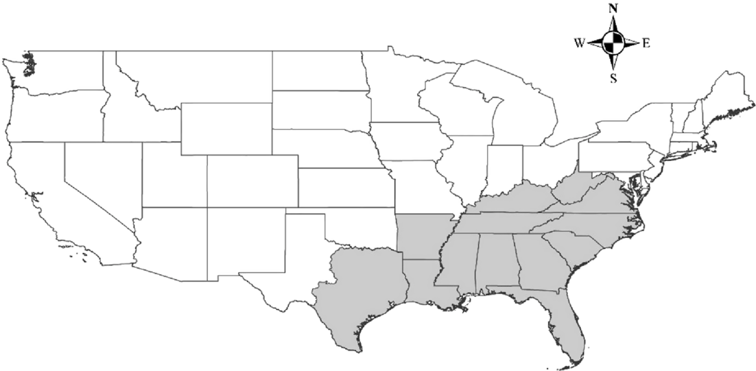
The study area corresponded to the shaded region shown in Figure 1. We selected this region because it covers all of the states in the U.S. Forest Service (USFS) Region 8 (Southern Region), with two exceptions. West Virginia was added to increase the coverage of Appalachian forest, which is present in parts of seven states within USFS Region 8. Western Texas was excluded from our study area, because it includes a diversity of ecosystem types not found throughout the remaining USFS Region 8 states. The vast area of the southeastern United States represented in the present work is greatly affected by human activities such as agriculture, silviculture, and urbanization and has a wide variety of climatic and topographic conditions.

Figure 1. Study area. Continuous lines delimitate U.S. states. The shaded area indicates the region selected for the project.
Species Data
We used the Web-based mapping system EDDMapS (Early Detection and Distribution Mapping System) to obtain the occurrence points of 45 major invasive plant species causing negative effects in the study area (Table 1), which is an area of primary concern with regard to the spread of invasive exotic plant species (Oswalt and Oswalt Reference Oswalt and Oswalt2011). The species data were collected between 2007 and 2018 and were downloaded in February 2018. We selected only verified and positive observations of those invasive species, which included locations where the species have been found, treated, and/or eradicated.
Table 1. Relative contribution (permutation importance) of the environmental variables to develop the maximum entropy (MaxEnt) models, percent of the study area that is at risk for species invasions (invasion risk > 10 percentile training presence Cloglog threshold), and evaluation of model performance with the area under the receiver operator characteristic curve (AUC) and the true skill statistic (TSS).a
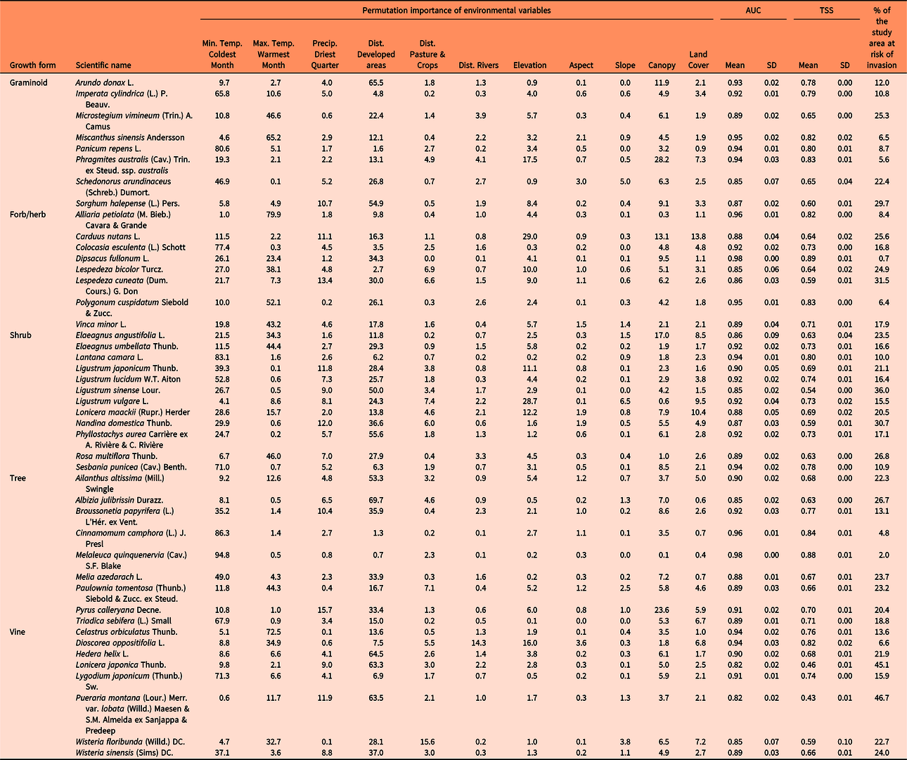
a Higher values of both AUC and TSS indicate better performance of a model, with maximum value of +1 for each.
The occurrence points of the invasive species analyzed were spatially aggregated, which indicates the possible presence of spatial autocorrelation in the sample data. If spatial aggregation of occurrence records implies spatial autocorrelation in the data, the assumption of independence between records will be violated, leading to inflated Type I error rates, problems with the significance of test statistics, and diminished predictive performance (Dormann et al. Reference Dormann, McPherson, Araújo, Bolliger, Carl, Davies, Hirzel, Jetz, Kissling, Kühn, Ohlemüller, Peres-Neto, Reineking, Schroder, Schurr and Wilson2007; Fielding and Bell Reference Fielding and Bell1997; Legendre Reference Legendre1993). Thus, to avoid spatial autocorrelation and following what other authors have done in large-scale studies (e.g., Catford et al. Reference Catford, Vesk, White and Wintle2011), we randomly selected occurrence points that were separated by at least 10 km.
Since its launching by the Center for Invasive Species and Ecosystem Health at the University of Georgia in 2005, EDDMapS has recorded more than 3.3 million invasive species observations made by different individuals, institutions, and environmental organizations such as universities, herbaria, the U. S. Forest Service (USFS), the U.S. Department of Agriculture (USDA), and the Nature Conservancy (EDDMapS 2018). Also, EDDMapS indicates which records have been verified by experts, making it a robust and reliable data set (EDDMapS 2018). Data within the EDDMapS application represent a mix of occurrence points drawn from experimental or systematically designed observational studies, along with data that were collected more opportunistically in easily accessed areas. This could influence the model results such that they reflect sampling effort rather than habitat selection by the species of interest (Phillips et al. Reference Phillips, Dudík, Elith, Graham, Lehmann, Leathwick and Ferrier2009). With this in mind, we partially controlled for potential biases associated with a disproportionate number of occurrence points clustered within a few discrete locations (usually near roads and populated areas) when we reduced spatial autocorrelation by using thinned occurrence points. Also, there were many occurrence points within forests and other land covers far from developed areas, suggesting adequate representation of occurrence data across a range of land use/land cover types.
Environmental Variables
We compiled a broad representation of geospatially explicit environmental variables related to climate, topography, land cover, land use, and propagule pressure that are likely to influence landscape susceptibility to invasion. We downloaded 19 grid-based bioclimatic variables from the Worldclim database (Fick and Hijmans Reference Fick and Hijmans2017), which includes the average for the years 1970 to 2000 at 30-arc second (~ 1 km2) resolution. Based on the importance of climate extremes in explaining spatial patterns (Zimmermann et al. Reference Zimmermann, Yoccoz, Edwards, Meier, Thuiller, Guisan, Schmatz and Pearman2009), we then selected what we perceived to be the three most biologically relevant bioclimatic variables that could potentially affect the establishment and spread of invasive species throughout the southeastern United States (minimum temperature of coldest month, maximum temperature of warmest month, and precipitation of driest quarter). Because the southeastern United States is a relatively humid area, we excluded precipitation of wettest quarter to reduce the number of variables that refer to similar environmental conditions. Minimum temperature of coldest month and maximum temperature of warmest month described the availability of thermal energy and the species thermal tolerance, whereas precipitation of driest quarter described the lowest water availability that the species can tolerate (Ficetola et al. Reference Ficetola, Thuiller and Miaud2007). We resampled the bioclimatic maps to a grid of 30-m resolution using the bilinear resample technique, which calculates the value of each pixel by averaging (weighted for distance) the values of the four nearest pixels (ESRI 2018). This resampling method is more accurate and less computationally intensive than other resample techniques and has been broadly implemented in ecological studies (Arif and Akbar Reference Arif and Akbar2005; Chapman et al. Reference Chapman, Muñoz and Koch2005).
We obtained land cover and percent tree canopy cover data from the National Land Cover Database (NLCD) 2011 (Homer et al. Reference Homer, Dewitz, Yang, Jin, Danielson, Xian, Coulston, Herold, Wickham and Megown2015), a data set created by the Multi-Resolution Land Characteristics Consortium. This raster layer has a spatial resolution of 30 m and includes categorical classification of vegetation types, developed areas, land use, barren areas, and open water. The percent tree canopy cover layer was developed from multispectral Landsat imagery and other available ground information (Homer et al. Reference Homer, Dewitz, Yang, Jin, Danielson, Xian, Coulston, Herold, Wickham and Megown2015).
We calculated Euclidean distance to the nearest pasture/cultivated area from the occurrence records using ArcGIS 10.5.1 (ESRI 2018). The same was applied to calculate the nearest distance to developed areas, a surrogate for propagule pressure. We downloaded road maps from 2017 from the Geography Division of the U.S. Census Bureau (USCB 2017) and calculated Euclidean distance to the nearest road. Distance to rivers has also been considered as a source of propagules in several instances (Catford et al. Reference Catford, Vesk, White and Wintle2011; Chytry et al. Reference Chytry, Vojtech, Pyseck, Hajek, Knollova, Lubomir and Danihelka2008). We obtained maps related to linear hydrography from the USCB (2017) and then calculated the Euclidian distance to rivers using ArcGIS 10.5.1 (ESRI 2018). We also downloaded digital elevation data at 100-m spatial resolution from 2013 from the U.S. Geological Survey (USGS 2017) and resampled to a grid of 30-m pixel size using the bilinear resample technique. Other topographic variables such as aspect and slope were derived from the elevation grid using ArcGIS 10.5.1 (ESRI 2018).
We retained noncorrelated environmental variables to predict the distribution of each invasive species in the study area. We excluded distance to roads in model development, because it was highly correlated with distance to developed areas (Pearson’s r = 0.86; sensu Catford et al. Reference Catford, Vesk, White and Wintle2011). The exclusion of distance to roads further reduced possible effects of sampling bias. After removing distance to roads, the highest Pearson’s r value was 0.45. We tested correlation between quantitative variables by extracting the information from background points randomly distributed throughout the study area and separated by at least 10 km to avoid spatial autocorrelation.
Model Development and Validation
We modeled the susceptibility of the 30-m resolution grid to be invaded by each invasive species using a maximum entropy (MaxEnt) modeling approach. MaxEnt is a robust technique for invasive species modeling and has been reported to be among the best distribution models in several occasions (Duan et al. Reference Duan, Kong, Huang, Fan and Wang2014; Elith et al. Reference Elith, Graham, Anderson, Ferrier, Guisan, Hijmans, Huettmann, Leathwick, Lehmann, Li, Lohmann, Loiselle, Manion, Moritz and Nakamura2006; Tognelli et al. Reference Tognelli, Roig-Junent, Marvaldi, Flores and Lobo2009). Furthermore, this machine-learning method provides good predictive power across different sample sizes (West et al. Reference West, Kumar, Brown, Stohlgren and Bromberg2016; Wisz et al. Reference Wisz, Hijmans, Li, Peterson, Graham and Guisan2008). We included in the MaxEnt models a broad set of environmental variables related to climate (minimum temperature of coldest month, maximum temperature of warmest month, and precipitation of driest quarter), topography (elevation, aspect, and slope), land cover, canopy, land use, and propagule pressure (distance to the nearest developed area, distance to the nearest pasture/cultivated area, and distance to rivers).
We used a 10-fold cross-validation procedure to test predictive power of the models and achieve a better model output. This method separates the occurrence points into equal-sized groups (folds), and every iteration leaves out one different fold, therefore using all of the data for validation (Phillips Reference Phillips2017). We retained the outputs that included the average and standard deviation of the replicates. Furthermore, we used the Cloglog (complementary log-log) output format, because it is considered to be the most appropriate for estimating relative suitability for colonization (Phillips et al. Reference Phillips, Anderson, Dudík, Schapire and Blair2017). For each model, we used 10,000 randomly generated pseudo-absence/background points distributed throughout the study area. The other parameters of MaxEnt remained at default.
We used permutation importance to evaluate the relative contribution of the different environmental variables to the distribution models. The permutation importance is determined by randomly permuting the values of each variable among the training points (both presence and pseudo-absence) and measuring the resulting decrease in training area under the curve (AUC). A large decrease indicates that the model depends heavily on that variable. Therefore, this measure depends only on the final MaxEnt model, not the path used to obtain it (Donald et al. Reference Donald, Gedeon, Collar, Spottiswoode, Wondafrash and Buchanan2012; Kalle et al. Reference Kalle, Ramesh, Qureshi and Sankar2013).
Model performance (the discrimination ability of the model or model’s goodness of fit) was evaluated using the AUC of the receiver operator characteristic (ROC) plot (Franklin Reference Franklin2009) and the true skill statistic (TSS). AUC values are provided by the MaxEnt model output and range from 0 to 1. Higher AUC values indicate better performance of the model (Peterson et al. Reference Peterson, Soberón, Pearson, Anderson, Martinez-Meyer, Nakamura and Araujo2011). The TSS considers both sensitivity and specificity. Sensitivity measures the percentage of correctly classified presences, while specificity measures the percentage of correctly classified absences (West et al. Reference West, Kumar, Brown, Stohlgren and Bromberg2016), or in the case of this project, pseudo-absences. The TSS ranges from −1 to 1, with values of 0 or less representing that the model is no different from random, whereas a value of +1 indicates 100% agreement of the model with the data. Thus, the TSS was calculated with the values of sensitivity and specificity that resulted from counting the number of cells with values above or below the “10 percentile training presence Cloglog threshold” in both background and sample predictions provided by the MaxEnt model output. The TSS was calculated for every replicate and then averaged by species.
Landscape Characteristics and Susceptibility to Invasion
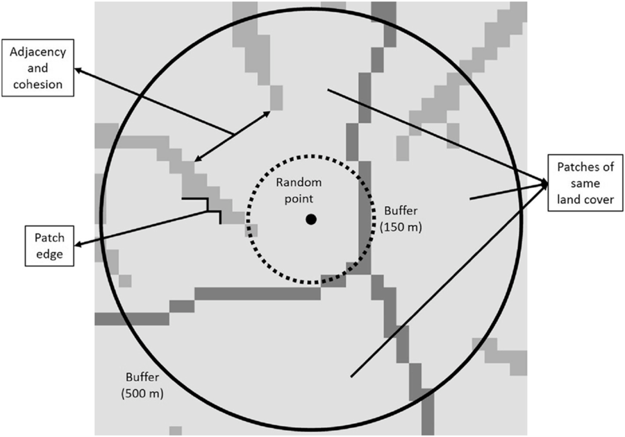
We extrapolated predictions resulting from the MaxEnt models to provide maps of invasion risk at 30-m resolution for the southeastern United States. To examine the relationship between landscape characteristics and susceptibility to invasion at different spatial scales, we placed random points in the resulting invasion risk maps and followed the next approach. We separated the random points by 10 km to avoid spatial autocorrelation issues, and to interpret the results clearly, we placed the random points within an area that included the distributional range of the occurrence points of each species, plus a buffer of 25 km from the distribution limit. To assess the landscape characteristics around the random points, we created two buffers around those points at different distances: medium (0 to 150 m) and long (0 to 500 m) using the function gBuffer of the rgeos package in the program R (R Core Team 2018). We evaluated landscape composition and configuration using NLCD 2011 (Homer et al. Reference Homer, Dewitz, Yang, Jin, Danielson, Xian, Coulston, Herold, Wickham and Megown2015) and within the abovementioned buffers using the ClassStat function of the SDMTools package.
Landscape composition refers to the proportion of the landscape occupied by the different land cover types, which were divided into seven categories: (1) forest (evergreen, deciduous, mixed forests, and forested wetland), (2) shrub/scrublands, (3) herbaceous wetland, (4) pasture and grassland, (5) cultivated area, (6) developed area, and (7) barren land (Homer et al. Reference Homer, Dewitz, Yang, Jin, Danielson, Xian, Coulston, Herold, Wickham and Megown2015). Landscape configuration, in contrast to landscape composition, deals with the spatial arrangement of the different landscape elements that make up a given mosaic landscape. In this study, we evaluated (1) patch density (number of patches in the landscape, divided by total landscape area), (2) edge density (sum of the lengths of all edge segments in the landscape, divided by the total landscape area), (3) landscape shape index (total length of edge in the landscape divided by the minimum total length of edge possible), (4) proportion of like adjacencies (frequency with which different pairs of patch types (including like adjacencies between the same patch type) appear side by side), (5) aggregation index (similar to proportion of like adjacencies, but here each class is weighted by its proportional area in the landscape), (6) patch cohesion index (measures the physical connectedness of the corresponding patch type), (7) proportional landscape core (portion of landscape not affected by edge effect), and (8) land cover heterogeneity (number of different land cover categories that make up the landscape; VanDerWal et al. Reference VanDerWal, Falconi, Januchowski, Shoo and Storlie2019; Figure 2).

Figure 2. Graphical representation of some of the variables used to calculate landscape composition and configuration metrics at medium (0–150 m) and long (0–500 m) distances around random points. The number and area occupied by patches of the same land cover were used to calculate heterogeneity and the proportion of the landscape occupied by the different land cover types, respectively. Adjacency and cohesion are related to the degree of aggregation of patch types, whereas patch edge deals with the amount of edge in the landscape.
Data Analysis
We evaluated the relative contribution of the different environmental variables to the distribution models based on the permutation importance, and we assessed the MaxEnt model adequacy using AUC and TSS values. The assessment table proposed by Sofaer et al. (Reference Sofaer, Jarnevich, Pearse, Smyth, Auer, Cook, Edwards, Guala, Howard, Morisette and Hamilton2019) to deliver SDMs and inform decision making can be found in Supplementary Table S1.
Then, we analyzed the relationship between the susceptibility to invasion of random points in the 30-m resolution grid by each invasive species and the compositional and configurational landscape metrics obtained from the buffers around those random points. To evaluate that relationship for landscape composition, we first categorized the randomly selected locations in high and low invasion risk, depending on whether their susceptibility to invasion was above or below the “10 percentile training presence Cloglog threshold,” respectively. We then calculated the proportion of each land cover category found in locations with high and low invasion risk and in their surrounding landscapes at medium (0 to 150 m) and long (0 to 500 m) distances (Supplementary Tables S2 and S3). Finally, we divided the proportions from locations with high invasion risk by those from locations with low invasion risk. Values above and below 1 indicated that the corresponding land cover had a high or low susceptibility to invasion, respectively. Also, values close to 1 indicated medium susceptibility to invasion.
As for configurational landscape metrics, we used the Spearman correlation (r) with the function cor.test(…, method = “spearman”) of the program R (R Core Team 2018) to test their effect on invasion risk of the random locations. Spearman correlation is a more robust method to evaluate linear relationships than Pearson correlation, because the latter is greatly influenced by outliers and highly skewed variables.
Finally, we calculated the percent of the study area that is at risk of invasion by each species. For this purpose, we divided the area with invasion risk higher than the “10 percentile training presence Cloglog threshold” by the total area and then multiplied the result by 100 to obtain the percentage. We obtained hotspots for predicted plant invasions by calculating the mean susceptibility to invasion across the evaluated species for each cell in the resulting risk maps.
Results and Discussion
SDM Model Outputs
The results of this study show that large areas of the southeastern United States are highly susceptible to being invaded by the plant species evaluated. Some species such as silktree (Albizia julibrissin Durazz.), Chinese privet (Ligustrum sinense Lour.), Japanese honeysuckle (Lonicera japonica Thunb.), and kudzu [Pueraria montana (Lour.) Merr. var. lobata (Willd.) Maesen & S.M. Almeida ex Sanjappa & Predeep] are likely to establish (and have established) throughout the region, whereas others will probably occupy specific areas (Figure 3). For example, the distribution of camphor tree [Cinnamomum camphora (L.) J. Presl], cogongrass [Imperata cylindrica (L.) P. Beauv.], and Japanese climbing fern [Lygodium japonicum (Thunb.) Sw.] will probably be limited to coastal areas of the Gulf and East Coasts of the United States. In contrast, species such as garlic mustard [Alliaria petiolata (M. Bieb.) Cavara & Grande], Oriental bittersweet (Celastrus orbiculatus Thunb.), autumn olive (Elaeagnus umbellata Thunb.), sericea lespedeza [Lespedeza cuneata (Dum. Cours.) G. Don], and Nepalese browntop [Microstegium vimineum (Trin.) A. Camus], will establish mainly in interior areas of the United States. Finally, the future distribution of punk tree [Melaleuca quinquenervia (Cav.) S.F. Blake] seems to be restricted to Florida under current climatic conditions.
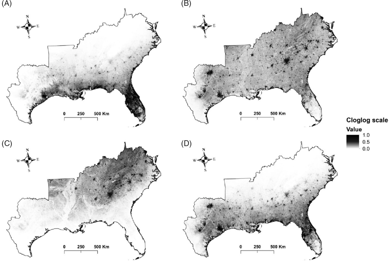
Figure 3. Invasion risk maps for: (A) Imperata cylindrica, (B) Lonicera japonica, (C) Microstegium vimineum, and (D) Triadica sebifera. The maps show the average output of 10 cross-validated maximum entropy (MaxEnt) model runs. Cloglog (complementary log-log) scale represents an estimate of relative colonization suitability for the species of interest. Darker shading indicates higher risk of invasion, while lighter shading illustrates the opposite.
Furthermore, our models indicate that the species with the greatest potential to establish across southeastern United States (25% to 47 % of the area) are A. julibrissin, nodding plumeless thistle (Carduus nutans L.), L. cuneata, L. sinense, L. japonica, M. vimineum, sacred bamboo (Nandina domestica Thunb.), kudzu [P. montana var. lobata], multiflora rose (Rosa multiflora Thunb.), and Johnsongrass [Sorghum halepense (L.) Pers.] (Table 1). Finally, hotspots for plant invasions show that landscapes around developed areas are especially vulnerable to plant invasions (Figure 4). However, this result could be partially influenced by sampling bias toward more accessible areas, which could increase the influence of proximity to developed areas in biological invasions in our study. Some fraction of the data stored in EDDMapS comes from opportunistic observations of invasive species occurrences, while other data come from formal scientific studies. In preparing for these analyses, we thinned the data by randomly selecting occurrence points that were separated by no less than 10 km. We expected that this would greatly reduce the impacts of roadside sampling, which is a typical result of opportunistic sampling for invasive species occurrence. This effort was reflected in the resulting models for 40% of our species, which showed higher affinities for habitat isolated from human activities, such as forest interiors and herbaceous wetlands.
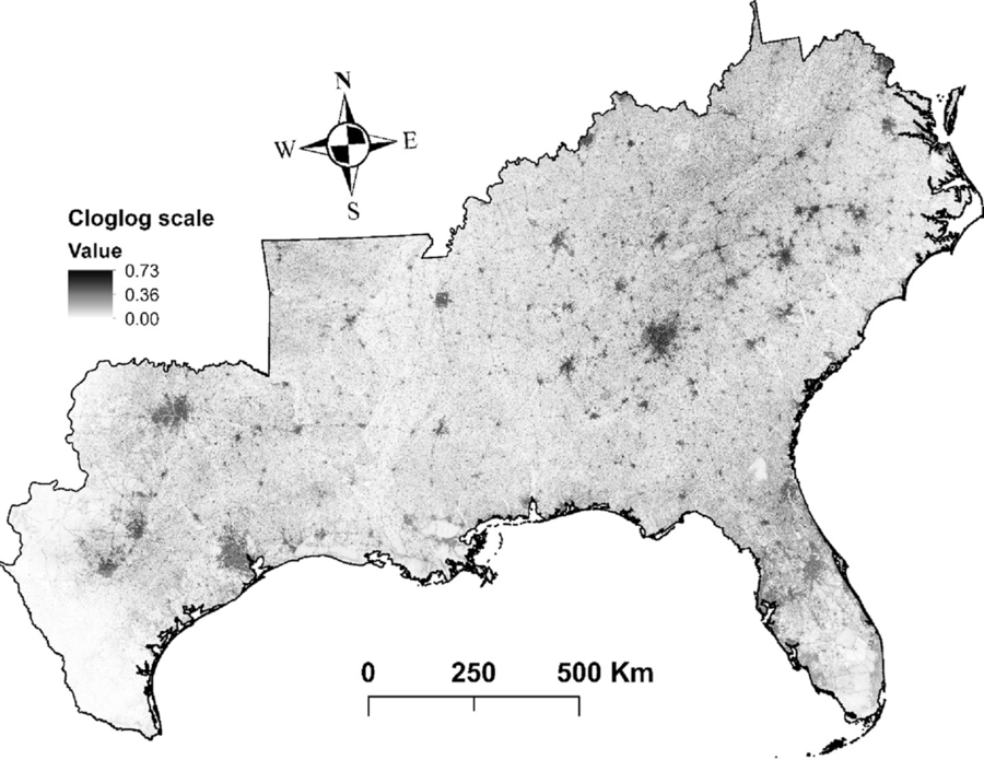
Figure 4. Hotspots for predicted plant invasions. This map represents the average susceptibility to invasion across all the species for each pixel. Cloglog (complementary log-log) scale represents an estimate of relative colonization suitability for the species of interest. Darker shading indicates higher risk of invasion, while lighter shading illustrates the opposite.
Model Performance Evaluation
The high average values of the 10-fold cross-validated AUCs and TSSs indicate that the MaxEnt models developed in this study exhibited good performance and thus had the ability to discriminate between presences and pseudo-absences (background) of our target species (Table 1). However, AUC and TSS values both declined substantially as the number of observations per species increased (Pearson r values: −0.44 and −0.51 for AUC and TSS, respectively). Because all species had the same number of pseudo-absence points (10,000), this relationship between model performance metrics and number of observations likely reflects an effect of the ratio of presence to pseudo-absence points. As noted in the “Introduction,” another concern with SDMs is that they may be less effective in modeling recently introduced invasive species, that is, species that are not yet at equilibrium with their new ranges. Most of the species in this study were introduced to the United States during the 1800s or early 1900s (only two with less than ~100 years since introduction), with some exceptional introductions in the 1700s (EDDMapS 2018). To assess the potential impact of recency of introduction on these models, we developed additional linear regression models between time since introduction and model adequacy for both AUC and TSS. We did not find any significant statistical correlation between time since introduction and AUC (P = 0.66; adjusted R-squared = 0) or TSS (P = 0.52; adjusted R-squared = 0).
Relative Contribution of the Environmental Variables
As expected, variables related to temperature were important in predicting the susceptibility of the 30-m resolution grid to be invaded by invasive plant species in the southeastern United States (Table 1). Plants are adapted to withstand certain temperature ranges, which vary depending on the species (Sakai et al. Reference Sakai, Allendorf, Holt, Lodge, Molofsky, With, Baughman, Cabin, Cohen, Ellstrand, McCauley, O’Neil, Parker, Thompson and Weller2001). Extreme temperatures, such as minimum temperature of coldest month and maximum temperature of warmest month, are likely to restrict the area where a given species can establish (Zimmermann et al. Reference Zimmermann, Yoccoz, Edwards, Meier, Thuiller, Guisan, Schmatz and Pearman2009). Precipitation of the driest quarter was less important than temperature, which could be due to the absence of an important hydric deficit period throughout the relatively humid southeastern United States, as well as due to relatively similar hydrological regimes in the driest quarter of the year across the original distributional ranges of the species. However, the importance of climatic variables in predicting susceptibility to invasion could be affected by limiting the study area to the southeastern United States. Several species evaluated in this study occupy large areas outside the southeastern United States, which leads to variation in temperature and precipitation regimes throughout their distributional ranges. Thus, the results of this study could differ if the SDMs were developed using all the areas occupied by such species in the United States (see, e.g., Yates et al. Reference Yates, Bouchet, Caley, Mengersen, Randin, Parnell, Fielding, Bamford, Ban, Barbosa, Dormann, Elith, Embling, Ervin and Fisher2018).
Distance to developed areas was the other main factor, along with temperature, that most contributed to invasion susceptibility. Developed areas are an important source of propagules and provide suitable habitat for many invasive exotic species, which are often planted in those areas for soil stabilization (Brown and Sawyer Reference Brown and Sawyer2012) and ornamental and aesthetic purposes (Säumel and Kowarik Reference Säumel and Kowarik2010). However, the possible effects of sampling bias toward more accessible areas such as roadsides could have increased the influence of distance to developed areas on our SDMs (Fournier et al. Reference Fournier, White and Heard2019). Distance to rivers has also been considered as a source of propagules in several occasions (Catford et al. Reference Catford, Vesk, White and Wintle2011; Chytry et al. Reference Chytry, Vojtech, Pyseck, Hajek, Knollova, Lubomir and Danihelka2008); however, it was insignificant for most of the species evaluated. The same applies for distance to pastures and cultivated areas, where invasive exotic species are frequently planted to support improved cattle forage opportunities (Booth et al. Reference Booth, Murphy and Swanton2003) or are established from seed or propagule contaminants in hay or other supplemental feeds (e.g., Conn et al. Reference Conn, Stockdale, Werdin-Pfisterer and Morgan2010) or dispersed by the cattle themselves (Mullahey et al. Reference Mullahey, Shilling, Mislevy and Akanda1998).
Canopy cover had a medium contribution to predict the models for most of the species, but it had a major role for some, including European common reed [Phragmites australis (Cav.) Trin. ex Steud. ssp. australis], C. nutans, Russian olive (Elaeagnus angustifolia L.), and Callery pear (Pyrus calleryana Decne.). Canopy cover and tree biomass have been considered one of the main factors that affect the distribution of exotic species in some parts of the study area (AL-L and GNE, personal observation; Iannone et al. Reference Iannone, Potter, Hamil, Huang, Zhang, Guo, Oswalt, Woodall and Fei2016). Finally, even though other studies have shown that topographic variables influence the establishment and spread of invasive species (e.g., Pauchard and Alaback Reference Pauchard and Alaback2004; Rouget and Richardson Reference Rouget and Richardson2003), they were insignificant to predict the susceptibility to invasion in our study area, with the exception of altitude, which had a secondary role. Most of the parts of southeastern United States have a relatively low topographic relief, which lowers the effect of slope and aspect on many species distributions.
Landscape Composition and Susceptibility to Invasion
The results of this study suggest, as expected, that human-disturbed systems are more prone to invasion than areas that experience minimal human interference. This pattern was consistent throughout the different spatial scales considered in this study. Developed areas were the land cover most vulnerable to exotic plant invasion (Table 2; Supplementary Table S4). Developed areas are land covers with some degree of impervious surfaces and include roadsides; parks; and residential, industrial, and urban areas (Homer et al. Reference Homer, Dewitz, Yang, Jin, Danielson, Xian, Coulston, Herold, Wickham and Megown2015). Developed areas are usually subjected to periodic disturbances that generate opportunities for plant colonization and establishment. Roadsides have been proven to be important habitat and/or corridors for exotic plant species globally (Lázaro-Lobo and Ervin Reference Lázaro-Lobo and Ervin2019). Barren lands, or areas where vegetation generally accounts for less than 15% of total cover (Homer et al. Reference Homer, Dewitz, Yang, Jin, Danielson, Xian, Coulston, Herold, Wickham and Megown2015), also had a high risk of invasion. Invasive species are successful colonizers of areas deprived of vegetation because of their broad ecological tolerances and ability to withstand harsh environments where other species cannot become established.
Table 2. Number of species with high, medium, and low susceptibility of invasion for each land cover type and spatial scale (location of evaluated points, medium distance, and long distance). a
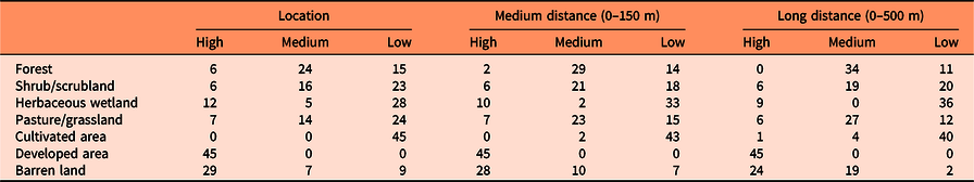
a The susceptibility of each land cover category to be invaded by each species was obtained by dividing the proportion of the corresponding land cover category found in locations with high invasion risk by that from locations with low invasion risk (see Supplementary Tables S2–S4 for details). Values above 1.25, between 0.75 and 1.25, and below 0.75 were considered as high, medium, and low susceptibility of invasion.
The remaining land cover types had generally moderate or low invasion risk. Although our results suggest that current distributions of only a few species of different growth forms are correlated with grasslands and pastures (e.g., S. halepense, tall fescue [Schedonorus arundinaceus (Schreb.) Dumort.], C. nutans, E. angustifolia, and P. calleryana), we believe that alterations of the ecological processes that sustain these herbaceous ecological systems, such as fire regimes or herbivory pressure, especially in the absence of monitoring efforts, would allow for the invasion of other exotic species, as has been shown by many previous studies. Shrub/scrublands include areas with shrubs and young trees in an early successional stage (Homer et al. Reference Homer, Dewitz, Yang, Jin, Danielson, Xian, Coulston, Herold, Wickham and Megown2015). The invasive species that were predicted to be more likely to occupy this land cover are I. cylindrica, shrub lespedeza (Lespedeza bicolor Turcz.), L. japonicum, and Chinese wisteria [Wisteria sinensis (Sims) DC.]. Cultivated areas demonstrated the lowest risk of invasion. Those areas are generally actively managed to maximize crop yields, which may impede the establishment of colonizing plant species. However, because invasive species readily colonize abandoned fields (Kulmatiski et al. Reference Kulmatiski, Beard and Stark2006; Mosher et al. Reference Mosher, Silander and Latimer2009), we believe that those areas would be prone to invasion once active management ceases.
The soil of herbaceous wetlands is periodically saturated with or covered with water (Homer et al. Reference Homer, Dewitz, Yang, Jin, Danielson, Xian, Coulston, Herold, Wickham and Megown2015), which is a handicap for some terrestrial invasive species. However, some species can become established when the substrate is unsaturated and are capable of surviving subsequent soil inundations for certain periods of time (King and Grace Reference King and Grace2000). In this sense, we found that species such as torpedo grass (Panicum repens L.), P. australis ssp. australis, A. petiolata, I. cylindrica, coco yam [Colocasia esculenta (L.) Schott], and M. quinquenervia were likely to colonize herbaceous wetlands. We found that a high proportion of locations with high risk of invasion corresponded to forested areas (Supplementary Table S2). One possible explanation for this finding is that forests are widely spread throughout the southeastern United States (Homer et al. Reference Homer, Dewitz, Yang, Jin, Danielson, Xian, Coulston, Herold, Wickham and Megown2015), and therefore, random points are more likely to be placed in this land cover. However, this proportion was outnumbered by the number of locations with low risk of invasion for most of the species (Supplementary Table S3), and only a few of them, such as M. vimineum, common periwinkle (Vinca minor L.), N. domestica, C. camphora, and Japanese wisteria [Wisteria floribunda (Willd.) DC.], were predicted to invade forests (probably highly managed forests). Previous research shows that these species are often found invading forests in the southeastern United States (e.g., DeMeester and Richter Reference DeMeester and Richter2010; Oswalt et al. Reference Oswalt, Oswalt and Clatterbuck2007; Trusty et al. Reference Trusty, Lockaby, Zipperer and Goertzen2007).
Furthermore, the vulnerability to invasion of the different land covers was consistent across the three spatial scales considered in this study (location and 0 to 150 m and 0 to 500 m from location), which suggest that the landscape did not have dramatic changes within a 500-m buffer from the random points. However, this result could be influenced by the high importance of climatic variables in our study, which were downloaded at an ~1-km2 resolution and resampled using the bilinear resample technique. Thus, most raster cells included within a buffer of 500 m from the occurrence point locations would have similar climatic values, and therefore, susceptibility to invasion would remain relatively constant.
Landscape Configuration and Susceptibility to Invasion
Susceptibility to invasion was highly correlated with configurational landscape metrics for most of the species (Table 3). However, the species I. cylindrica, C. esculenta, rattlebox [Sesbania punicea (Cav.) Benth.], and M. quinquenervia were not affected by any variable related to landscape configuration (Supplementary Table S5).
Table 3. Number of species with positive, neutral, or negative Spearman correlations (based on P-value < 0.001) between susceptibility to invasion of randomly selected locations and landscape configuration variables at medium (0–150 m) and long (0–500 m) distances from those locations (see Supplementary Table S5 for details).
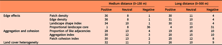
Generally, locations most vulnerable to exotic plant invasion (especially shrubs and vines) were predicted to be within landscapes with high edge or patch density and with low proportion of landscape core, as shown by previous research (e.g., Riitters et al. Reference Riitters, Potter, Iannone, Oswalt, Fei and Guo2017; Vilà and Ibáñez Reference Vilà and Ibáñez2011). However, some species showed the opposite pattern in at least one of the spatial scales, such as Chinese silvergrass (Miscanthus sinensis Andersson), P. repens, A. petiolata, and C. orbiculatus. This finding suggests that landscape heterogeneity benefits most of the major terrestrial invasive species that affect the southeastern United States (Melbourne et al. Reference Melbourne, Cornell, Davies, Dugaw, Elmendorf, Freestone, Hall, Harrison, Hastings, Holland, Holyoak, Lambrinos, Moore and Yokomizo2007), but some of them prefer more homogeneous landscapes.
Landscape metrics that measure the degree of aggregation and cohesion of patch types (proportion of like adjacencies, aggregation index, and patch cohesion index) generally had a positive relationship with susceptibility to invasion, which indicates that the presence of corridors for the dispersal of propagules highly influences landscape susceptibility to invasion (Lázaro-Lobo and Ervin Reference Lázaro-Lobo and Ervin2019; With Reference With2002). Yet some species, such as M. vimineum, M. sinensis, P. repens, A. petiolata, Japanese knotweed (Polygonum cuspidatum Siebold & Zucc.), E. umbellata, lantana (Lantana camara L.), C. orbiculatus, Chinese yam (Dioscorea oppositifolia L.), and W. floribunda, prefer landscapes with patches less aggregated and connected, especially at higher spatial scales (0 to 500 m). Also, landscape metrics related to aggregation and cohesion usually had a smaller impact on invasion risk than variables related to the amount of edge in the landscape.
Heterogeneity is a very important factor within a landscape. Heterogeneous landscapes enhance the biotic community that inhabits the area (Katayama et al. Reference Katayama, Amano, Naoe, Yamakita, Komatsu, Takagawa, Sato, Ueta and Miyashita2014; Ricketts and Sandercock Reference Ricketts and Sandercock2016), but when the heterogeneity is driven by anthropogenic modifications to the landscape, heterogeneity may increase a community’s susceptibility to invasion. In part, this results from human-assisted dispersal, but it also can result from the creation of available habitat space for the introduced species to occupy (Melbourne et al. Reference Melbourne, Cornell, Davies, Dugaw, Elmendorf, Freestone, Hall, Harrison, Hastings, Holland, Holyoak, Lambrinos, Moore and Yokomizo2007). In our study, susceptibility to invasion was significantly positively correlated with land cover heterogeneity for the majority of the species, (especially shrubs, trees, and vines), but there were a considerable number of species of different growth forms that did not show this pattern, especially at higher spatial scales (0 to 500 m). Therefore, this finding suggests that the influence of land cover heterogeneity on invasion risk is species specific.
In summary, our modeling approach allows for the delineation of areas in the southeastern United States likely to be invaded by major terrestrial invasive plant species. Conservation and restoration efforts should consider areas at high risk of invasion in their management plans, especially in “natural” areas with species and ecosystems of conservation concern. This study shows that human-disturbed systems such as developed areas and barren lands are more prone to be invaded than areas that experience minimal human interference; however, several invasive species are likely to colonize other land covers, depending on their individual ecological niches. We note, however, that for some species, this result could be partially influenced by sampling bias toward more accessible areas such as roadsides, which could increase the influence of proximity to developed areas in biological invasions within our study area. Another important finding is that even though landscape heterogeneity and the presence of corridors for propagule dispersal significantly increase landscape susceptibility to invasion for most of the species evaluated, there were a considerable number of species whose ability to invade increased in landscapes with large core areas and/or less-aggregated patches. Therefore, we conclude that even though we found general patterns for susceptibility to invasion, the influence of landscape composition and configuration on invasion risk was species specific.
Supplementary material
To view supplementary material for this article, please visit https://doi.org/10.1017/inp.2020.21
Acknowledgments
We would like to thank the Center for Invasive Species and Ecosystem Health of the University of Georgia for preparing the data that were downloaded from the EDDMapS web page. We are also grateful to the Quantitative Ecology and Spatial Technologies lab at Mississippi State University for use of their computers to develop the MaxEnt models and to Jean-François Gout for assistance with the supercomputer to analyze the landscape characteristics more efficiently. We are also grateful for many helpful suggestions provided by Catherine Jarnevich and two anonymous reviewers. This work was supported in part by USDA Forest Service grant 19-DG11083150-006. No conflicts of interest have been declared.