


I. INTRODUCTION
Gyrotropic media whose electric permittivity and magnetic permeability are tensors have peculiar optical and electromagnetic properties. They are distributed widely in the natural world such as the ionosphere. They have also been used as microwave devices such as circulators, isolators, resonators, and optical devices such as modulators, switches, phase shifters, etc. Therefore, it is necessary to study extensively wave propagation in a gyrotropic medium.
A large number of publications have been devoted to studying the characterizing interactions of electromagnetic waves in general gyrotropic materials in the past 20 years. Many analytical and numerical methods (e.g. the finite-difference time-domain (FDTD) method [Reference Hunsberger, Luebbers and Kuru1], the eigenfunction theory [Reference Barkeshli2, Reference Zhang, Li, Yeo and Leong3], the Dyadic Green's function [Reference Li, Leong and Kong4], the moment method (MM), etc.) have been applied. Several solutions have been reported on the two-dimensional scattering by gyrotropic spheres and circular cylinders. Electromagnetic scattering by a multilayer circular gyrotropic bianisotropic cylinder has been discussed in [Reference Zhang, Li, Yeo and Leong3, Reference Zhang, Yeo, Li and Leong5]. Electromagnetic fields in general gyrotropic media have been solved by using the method of separation of variables in [Reference Qiu, Li and Yeo6]. Okamoto has proposed a method based on the extended integral equation and showed the scattering properties of a circular ferrite cylinder and an elliptic ferrite cylinder [Reference Okamoto7, Reference Okamoto8]. Geng has treated electromagnetic scattering by an inhomogeneous plasma anisotropic sphere and spherical shell [Reference Geng, Wu and Li9, Reference Geng10].
However, these papers are only concerned with plane wave incidence. For some practical electromagnetic scattering problems, a Gaussian beam or a spherical wave is more realistic instead of a plane wave. The problem of scattering of a Gaussian beam by a homogeneous gyrotropic circular cylinder has been treated in this paper. A Gaussian beam approximate expression [Reference Kozaki11, Reference Tao, Wenbin and Sun12] is introduced to describe the accurate prediction of scattering behaviors, while the plane wave scattering is only its special case. In the expressions for the electromagnetic fields, the time dependence exp (jωt) is omitted throughout.
II. FORMULATION
As can be seen from Fig. 1, a cross-section of an infinitely long gyrotropic cylinder is shown. Two rectangular coordinate systems and one cylindrical coordinate system are defined. The z-axis, which is common to three coordinate systems, is not plotted. A Gaussian beam source, which is located at (x 1 = −ρ 0, y 1 = 0) is incident on the circular cylinder, making an angle θ 0 clockwise with respect to the negative x-axis.

Fig. 1. Geometry of the problem.
Consider a homogeneous gyrotropic cylinder characterized by the following permittivity and permeability tensors:
 $$\eqalign{ \bar{\bar{\varepsilon}} & = \left[ {\matrix{ {\varepsilon _{xx}} & { - j\varepsilon _{xy}} & 0 \cr {j\varepsilon _{xy}} & {\varepsilon _{xx}} & 0 \cr 0 & 0 & {\varepsilon _{zz}} \cr}} \right], \; \bar{\bar{\mu}} \cr & = \left[ {\matrix{ {\mu _{xx}} & { - j\mu _{xy}} & 0 \cr {j\mu _{xy}} & {\mu _{xx}} & 0 \cr 0 & 0 & {\mu _{zz}} \cr}} \right].}$$
A) Transmitted wave
Only the case of transverse-electric (TE) polarization is considered and the similar formulation of transverse-magnetic (TM) polarization can be obtained by adopting the similar method.
Referring to the Maxwell's equations, the differential equation for H-polarization inside a homogeneous gyrotropic cylinder (designated by the superscript c) is found to be
 $$\varepsilon _{xx}\left( {\displaystyle{{\partial ^2H_z^c} \over {\partial x^2}} + \displaystyle{{\partial ^2H_z^c} \over {\partial y^2}}} \right) + \omega ^2\mu _{zz}(\varepsilon _{xx}^2 - \varepsilon _{xy}^2 )H_z^c = 0.$$
The magnetic field
 $H_z^c $
can be written as follows [Reference Monzon and Damaskos13]:
$H_z^c $
can be written as follows [Reference Monzon and Damaskos13]:
 $$H_z^c (x,y) = \int_{C_\alpha} {d\alpha f(\alpha, \beta (\alpha ))} e^{\,j(\alpha x + \beta (\alpha )y)},$$
where f(α, β(α)) is the angular spectrum amplitude, α and β(α) denote the coefficients to be determined. Substitute equation (3) into (2), and equation (2) can be written as
 $$\alpha ^2 + \beta ^2 = \displaystyle{{\omega ^2\mu _{zz}(\varepsilon _{xx}^2 - \varepsilon _{xy}^2 )} \over {\varepsilon _{xx}}}.$$
If we set α = k 1cos ξ, β = k 1sin ξ, we have
 $$k_1 = \omega \sqrt {\displaystyle{{\mu _{zz}(\varepsilon _{xx}^2 - \varepsilon _{xy}^2 )} \over {\varepsilon _{xx}}}}. $$
For x = ρcosθ, y = ρ sinθ, equation (3) can be expressed as
 $$H_z^c (\rho, \theta ) = \int_{C_\xi} {d\xi H(\xi )} e^{\,jk_1\rho \cos (\theta - \xi )},$$
using the series expansion of plane wave [Reference Ren and Wu14]
 $$e^{jk_1\rho \cos (\theta - \xi )} = \sum\limits_{n = - \infty} ^\infty {j^{ - n}J(k_1\rho )e^{\,jn(\theta - \xi )}}, $$
and expanding H(ξ) in terms of the complete series expansion as follows:
 $$H(\xi ) = \sum\limits_{m = - \infty} ^\infty {C_me^{\,jm\xi}}. $$
Thus, the magnetic field in the circular cylinder region can be expressed as
 $$H_z^c (\rho, \theta ) = \sum\limits_{n = - \infty} ^\infty {j^{ - n}e^{jn\theta} \sum\limits_{m = - \infty} ^\infty {C_mH_{nm}(\rho )}}, $$
where
 $$H_{nm}(\rho ) = J_n(k_1\rho )\int_0^{2\pi} {e^{j(m - n)\xi} d\xi}, $$
where C m are unknown coefficients, J n (k 1 ρ) is the Bessel function of the first kind and order n.
B) Incident and scattered waves
The z-component of the magnetic field of the incident Gaussian beam source (designated by the superscript inc) is expressed as
 $$H_z^{inc} (x_1 = - \rho _0,y_1) = e^{ - \beta ^2y_1^2}, $$
where
 $$\beta ^2 = a_0^2 + jb_0^2, $$
where 1/|β| corresponds to the beamwidth of the incident wave.
The incident field from the source can be approximately expanded as [Reference Kozaki11]
 $$H_z^{inc} (\rho, \theta ) = \sum\limits_{n = - \infty} ^\infty {A_nj^{ - n}J_n(k\rho )e^{jn(\theta + \theta _0)}}, $$
where
 $$\!\!\eqalign{A_n & = \displaystyle{{e^{ - jk\rho _0}} \over {\sqrt {1 - jZ_0} }}e^{ - {\left( {{{n\beta } \over k}} \right)}^{\! \!2}{1 \over {1 - jZ_0}}} \cr & \quad \times \left[ {1 - 2{\left( {\displaystyle{\beta \over {k\sqrt {1 - jZ_0} }}} \right)}^4n^2 + \displaystyle{4 \over 3}{\left( {\displaystyle{\beta \over {k\sqrt {1 - jZ_0} }}} \right)}^6n^4 + \cdots } \!\right], \cr Z_0 & = \displaystyle{{2\beta ^2\rho _0} \over k}.} $$
k is the free-space wavenumber. This expression is valid for |(βλ)2| <0.3 and (a/λ) <5.0, where a is the radius of the cylinder.
The scattered magnetic field (designated by the superscript s) in the free space region is expressed as
 $$H_z^s (\rho, \theta ) = \sum\limits_{n = - \infty} ^\infty {B_nj^{ - n}H_n^{(2)} (k\rho )e^{jn\theta}}, $$
where B
n
are unknown coefficients and
 $H_n^{(2)} $
is the Hankel function of the second.
$H_n^{(2)} $
is the Hankel function of the second.
C) Boundary conditions
The tangential components of the electric and magnetic fields are continuous on the surface of the gyrotropic circular cylinder. Assume that the surface is represented by ρ = a, and thus the boundary conditions on the gyrotropic-free space interface are given by
 $$H_z^c = H_z^{inc} + H_z^s, \;\rho = a,$$
 $$E_\theta ^c = E_\theta ^{inc} + E_\theta ^s, \;\rho = a.$$
The tangential component of the electric field on the inner side of the interface of gyrotropic-free space can be expressed as
 $$j\omega \gamma E_\theta ^c = - \left[ {\varepsilon _{xx}\displaystyle{{\partial H_z^c} \over {\partial \rho}} + j\varepsilon _{xy}\displaystyle{1 \over \rho} \displaystyle{{\partial H_z^c} \over {\partial \theta}}} \right],$$
where
 $\gamma = \varepsilon _{xx}^2 - \varepsilon _{xy}^2 $
, which can be simplified to
$\gamma = \varepsilon _{xx}^2 - \varepsilon _{xy}^2 $
, which can be simplified to
 $$E_\theta ^c (\rho, \theta ) = \sum\limits_{n = - \infty} ^\infty {j^{ - n}e^{\,jn\theta} \sum\limits_{m = - \infty} ^\infty {C_mE_{nm}(\rho )}}, $$
where
 $$\eqalign{ E_{nm}(\rho ) &= \displaystyle{{jk_\theta} \over {\omega \gamma}} \left[ {\varepsilon _{xx}{{J}^{\prime}}_n(k_\theta \rho ) - \varepsilon _{xy}\displaystyle{n \over {k_\theta \rho}} J_n(k_\theta \rho )} \right] \cr & \quad\int_0^{2\pi} {e^{j(m - n)\theta _m}d\theta _m},} $$
while the tangential component of the electric field on the outer side of the interface of gyrotropic-free space can be written as
 $$E_\theta ^{inc(s)} = \displaystyle{j \over {\omega \varepsilon _0}}\displaystyle{{\partial H_z^{inc(s)}} \over {\partial \rho}}, $$
 $$E_\theta ^{inc} (\rho, \theta ) = j\sqrt {\displaystyle{{\mu _0} \over {\varepsilon _0}}} \sum\limits_{n = - \infty} ^\infty {A_nj^{ - n}{{J}^{\prime}}_n(k\rho )e^{jn(\theta + \theta _0)}}, $$
 $$E_\theta ^s (\rho, \theta ) = j\sqrt {\displaystyle{{\mu _0} \over {\varepsilon _0}}} \sum\limits_{n = - \infty} ^\infty {B_nj^{ - n}H{_n^{(2)}} ^{\prime}(k\rho )e^{jn\theta}}. $$
Applying the boundary conditions (16) and (17), two equations can be obtained as
 $$\eqalign{& {2 \over {\pi ka}}A_ne^{\,jn\theta _0} = \sum\limits_{m = - \infty} ^{ + \infty} \cr & \qquad {C_m\left[ {jH{_n^{(2)}} ^{\prime}(ka)H_{nm}(a) - \sqrt {\displaystyle{{\varepsilon _0} \over {\mu _0}}} H_n^{(2)} (ka)E_{nm}(a)} \right]},}$$
 $$B_n = \displaystyle{1 \over {H_n^{(2)} (ka)}}\left[ {\sum\limits_{m = - \infty} ^{ + \infty} {C_mH_{nm}(a)} - A_nJ_n(ka)e^{jn\theta _0}} \right].$$
In order to obtain numerical results, the infinite series needs to be truncated under the prerequisite of achieving the solution convergence. The unknown coefficients can be obtained from these equations finally, and the electromagnetic field can be calculated, while the radar cross-section (RCS) per unit length can be written as:
 $$\displaystyle{\sigma \over \lambda} (\theta, \theta ^{inc}) = \displaystyle{2 \over \pi} \left \vert {\sum\limits_{n = - \infty} ^{ + \infty} {B_ne^{jn\theta}}} \right \vert ^2.$$
III. NUMERICAL RESULTS
To check the validity and accuracy of the proposed method and the Fortran associated code, the plane wave incidence case is considered. Figure 2 shows the angular distributions of the normalized RCS per unit length for the plane wave case. For the sake of comparison, the results of Monzon and Damaskos [Reference Monzon and Damaskos13] and those of the FDTD method (the frequency of the incident wave is 1 GHz) are also shown in Fig. 2. For the plane wave incidence case, both a 0 and b 0 are set to be zero, while (ρ 0/λ) = 3.0, ka = π/2, θ inc = 180°. The elements in the permittivity tensor and the permeability tensor are: ε xx = 4.0ε0, ε xy = −2jε0, μ zz = 2μ 0. The results come into agreement with those comparison results for the plane wave incidence case.
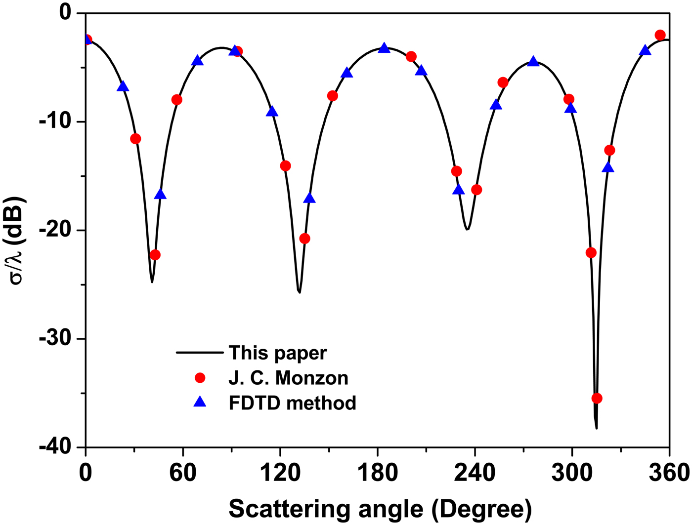
Fig. 2. H polarization, θ inc = 180°, ka = π/2, ε xx = 4.0ε0, ε xy = −2jε0, μ zz = 2μ 0.
Figure 3 illustrates an example with x and y principal axes for both Gaussian beam and plane wave incidence cases, with θ inc = 180°, ka = 2π, ε xx = 2ε0, ε xy = 0, μ zz = 2μ 0, and a 0 λ = 0.3, b 0 λ = 0.4 for the Gaussian beam. As one can see from this figure, the RCS is symmetrical around θ = 180° due to the symmetry of the cylinder around this angle. Figure 4 shows more general cases, with θ inc = 180°, ka = 2π, ε xx = 3ε0, ε xy = −1.5jε0, μ zz = 2μ 0, and a 0 λ = 0.3, b 0 λ = 0.4 for the Gaussian beam. The RCS is unsymmetrical in all the three cases because of the appearance of the parameter, ε xy . Unlike the uniform distribution property of plane wave, the scattering behavior of Gaussian beam is closely related to its beam optical source. The Gaussian beam backward scattering width is lower than the plane wave one. Because of the complexity of Gaussian beam scattering behaviors, many available EM commercial tools cannot give the numerical results directly for the Gaussian beam case. The comparison between the proposed method and those numerical solvers is left for a future discussion.
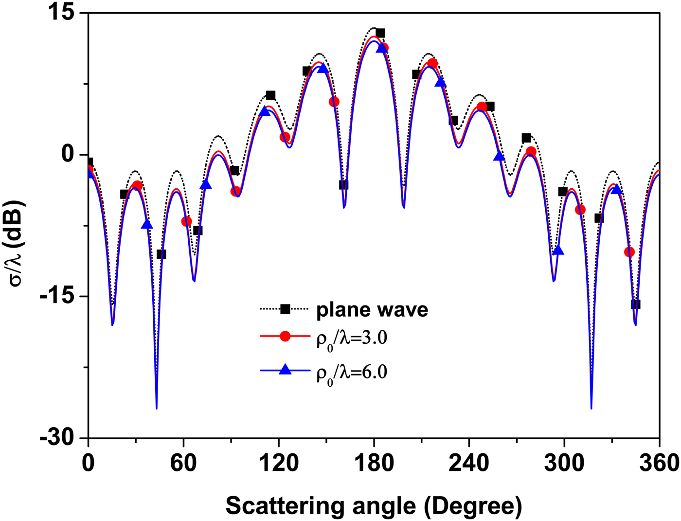
Fig. 3. H polarization, bistatic radar cross-sections d/λ dB, θ inc = 180°, ka = 2π, ε xx = 2ε0, ε xy = 0, μ zz = 2μ 0, a 0 λ = 0.3, b 0 λ = 0.4, N = 28.

Fig. 4. H polarization, bistatic radar cross-sections d/λ dB, θ inc = 180°, ka = 2π, ε xx = 3ε0, ε xy = −1.5jε0, μ zz = 2μ 0, a 0 λ = 0.3, b 0 λ = 0.4, N = 28.
IV. CONCLUSION
A solution to a Gaussian beam scattering properties from a homogeneous gyrotropic circular cylinder was presented. The solution was given for the TE case, and the TM case could be obtained via duality. The validity and accuracy of the numerical results were examined by making use of limiting cases such as the plane wave case. Several numerical results were given and discussed, which were of useful values for the development of approximate and numerical techniques as well as antennas and radar applications. The applications of the present formulation can be extended to include layered or elliptic cylinder structures [Reference Hamid and Cooray15] involving the gyrotropic medium.
ACKNOWLEDGEMENTS
The authors are greatly indebted to Professor J.-Mi. Jin for providing Bessel function subroutines on his website http://jin.ece.uiuc.edu/. This work was supported by the Natural Science Foundation of the Jiangsu Higher Education Institutions of China (Grant numbers 15KJB140009 and 16KJB460022).
 Shi-Chun Mao received his Ph.D. degree at Xidian University in 2010. His main research interests are electromagnetic and optical scattering.
 Zhen-Sen Wu received his M.Sc. degree at Wuhan University in 1981. He is currently a Professor at Xidian University. His research interests include electromagnetic and optical waves in random media, optical wave propagation and scattering, and ionospheric radio propagation.
 Zhaohui Zhang received his M.Sc. degree at Jiangsu Normal University. He is good at MD simulations and QC simulations, the main programs used are Fortran, LAMMPS, VMD, Gaussian, and MS.
 Jiansen Gao received his M.Sc. degree at Nanjing Normal University. His main research interest is Material physics.


