Introduction
Due to their special properties [Reference Viktor1–Reference Zhu, Liang and Li3], there has been an ever-increasing use of metamaterial-based components in the implementation of microwave devices such as couplers and filters. The metamaterial transmission line (TL) theory has been investigated by several research groups [Reference Oliner4–Reference Afrooz, Abdipour and Martin7].
The pure left-handed (LH) lines demonstrating backward-wave propagation are realized by cascaded series capacitances and shunt inductances. Since the LH structures are implemented on a host line making subsequent parasitic effects (corresponding to the line inductance and capacitance), the pure LH characteristics are not feasible in practical cases. Therefore, the concept of composite right-/left-handed (CRLH) TL including both the right-handed (RH) and LH parts is introduced which shows backward-wave propagation at low frequencies and forward-wave propagation at high frequencies (the RH characteristics). The most favored planar CRLH structures can be the series interdigital capacitors and shunt shorted stubs which offer simultaneously negative ε and μ [Reference Caloz and Itoh6, Reference Lai, Itoh and Caloz8], enabling decrease in size and potential performance improvement [Reference Lei, Caloz and Itoh9–Reference Danaeian, Afrooz and Hakimi12].
In conventional couplers, the compromise between bandwidth and coupling level has been a challenging task [Reference Mongia, Bhartia, Bahl and Hong13, Reference Pozar14]. In Lange couplers, both broad bandwidth and tight coupling can be achieved at the cost of bonding wires resulting in parasitic effects at high frequencies [Reference Lange15]. The CRLH couplers have also shown to provide broad bandwidth and tight coupling, and so can be used as alternatives to the conventional counterparts [Reference Caloz, Sanada and Itoh11, Reference Keshavarz, Movahhedi and Abdipour16]. Regarding this coupler as a multi-conductor TL (MCTL), coupled differential equations can be obtained that have no analytical solution, and so the numerical methods become very useful in such cases.
The full-wave analysis method which numerically solves the partial differential equations is rigorously accurate [Reference Hussein and El-Ghazaly17], but as a global modeling approach, it requires high CPU usage. Although, attempts have been made to decline the computational demand, it is still difficult to justify this approach in many practical cases [Reference Movahhedi and Abdipour18–Reference Mirzavand, Abdipour, Moradi and Movahhedi20] and this is where time-domain analysis has shown to be very efficient. The time-domain analysis of metamaterial TLs has been accomplished based on the method of moment and the Green's function method [Reference Zhang and Spielman21–Reference Gomez-Diaz, Gupta, Lvarez-melcon and Caloz23]. The finite-difference time-domain (FDTD) method as a versatile and easy-to-implement technique is successfully applied to numerical solutions. Recently, the CRLH TL has been analyzed based on the leap-frog (LF) FDTD method [Reference Afrooz, Abdipour and Martin7, Reference Ghadimi and Asadi24]. But the LF method is conditionally stable due to the Courant–Friedrichs–Lewy (CFL) constraint [Reference Taflove25].
On the other hand, the unconditionally stable implicit Crank–Nicolson FDTD (CN-FDTD) is similar to the LF scheme in terms of second-order accuracy in both space and time domain [Reference Thomas26, Reference Guilin and Trueman27]. The well-known CN-FDTD method has been efficiently applied to time-domain solution of Maxwell's equations and it has been more considerable by EM communication after 2000 [Reference Guilin and Trueman27–Reference Honarbakhsh and Asadi29]. In the CN method, selecting a larger time step size (Δt) leads to a remarkable decline in the CPU time compared with the conditionally stable methods. It should be mentioned that, the more Δt increases, the less accuracy is achieved [Reference Yang, Chen, Wang and Yung28, Reference Honarbakhsh and Asadi29]; thus, Δt should be selected considerately. In general, a huge sparse irreducible matrix arising from spatial discretization is inevitable in the CN-FDTD method, though this is not considered to be a negative consequence in one dimension (1D) along x (x being the direction of propagation) such as the problem at hand.
As the CN-FDTD method, the alternating direction implicit (ADI) FDTD is unconditionally stable [Reference Namiki30]. The CN-FDTD method has less numerical dispersion with respect to the ADI scheme [Reference Namiki30–Reference Garcia, Tae-Woo and Hagness32]; therefore, it is expected that this method supersedes the ADI-FDTD method very soon. Concerning the huge computational cost of the CN method for general 3D problems, to date some efforts have been made. For example, the locally 1D FDTD method shows more efficiency than that of the conventional ADI-FDTD method [Reference Lee and Fornberg33–Reference Liu, Chen and Yin35]. It should be mentioned that two unconditionally stable methods (other than the CN scheme) have been applied to analyze the MCTLs [Reference Kijun, Song Jae, Dong Chul and Yeon Choon36, Reference Afrooz and Abdipour37] and also single CRLH TL [Reference Afrooz, Abdipour and Martin7, Reference Afrooz38]. Yet, the application of the CN-FDTD method to a multi-conductor CRLH TLs has not been reported. As a result, the computational time gain and guarantying the efficient analysis of CRLH MCTLs are unknown in the said cases. Although applying the CN-FDTD method decreases the computation time in 1D, this scheme suffers from a huge sparse block banded matrices in 3D problems [Reference Yang, Chen, Wang and Yung28].
In the present study, a CRLH coupled-line coupler is studied in 1D. The CN-FDTD method is applied to this coupler, depicted in Fig. 1(a). The constituent unit cell is shown in Fig. 2(a). In “Results and discussion” section, the results are presented in time domain and also using the scattering parameters. In order to validate the CN-FDTD scheme, the accuracy and the time gain achieved from this method are compared with those of the LF scheme and the measurement.
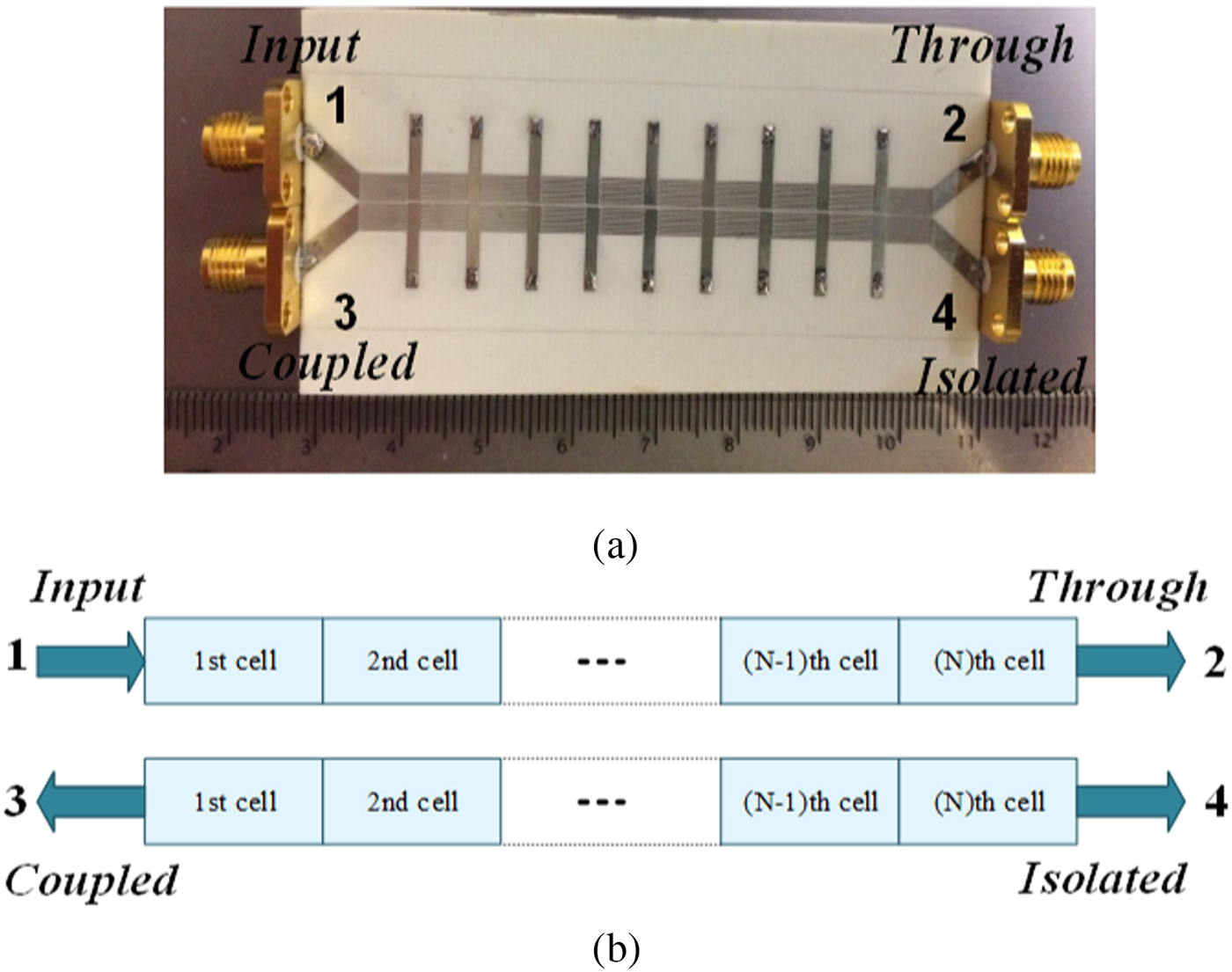
Fig. 1. (a) The fabricated coupler, (b) operational block diagram of a typical CRLH coupled-line coupler.

Fig. 2. (a) Layout of unit cell of fabricated coupler shown in Fig. 1(a), l 1 = 8 mm, l 2 = 2.4 mm, w 1 = 1.1 mm, w 2 = 5 mm, d = 0.6 mm, and its equivalent circuit model, and (b) the CRLH coupled unit cells and equivalent circuit model including the coupling capacitance C m and mutual inductance L m.
Mathematical approach
The block diagram of a typical CRLH coupled-line coupler consisting of two coupled CRLH TLs is depicted in Fig. 1(b) and the equivalent circuit model of one of coupled unit cells is shown in Fig. 2(b). For an infinitesimal line section with length Δx, applying the Kirchhoff's current and voltage laws to this unit cell leads to:
 $$\left\{ \matrix{\displaystyle{{\partial v_1} \over {\partial x}} + R^{{\kern 1pt} (1)}{\kern 1pt} {\kern 1pt} i_1 + L_R^{{\kern 1pt} (1)} \displaystyle{{\partial i_1} \over {\partial t}}{\kern 1pt} {\kern 1pt} + L_m\displaystyle{{\partial i_2} \over {\partial t}}{\kern 1pt} {\kern 1pt} + \displaystyle{{v_{C_L^{{\kern 1pt} (1)}}} \over {\Delta x}} = 0 \hfill \cr \displaystyle{{C_L^{{\kern 1pt} (1)}} \over {\Delta x}}\displaystyle{{\partial v_{C_L^{{\kern 1pt} (1)}}} \over {\partial t}}-i_1 = 0 \hfill \cr \displaystyle{{\partial v_2} \over {\partial x}} + R^{{\kern 1pt} (2)}{\kern 1pt} {\kern 1pt} i_2 + L_m\displaystyle{{\partial i_1} \over {\partial t}} + L_R^{{\kern 1pt} (2)} \displaystyle{{\partial i_2} \over {\partial t}} + \displaystyle{{v_{C_L^{{\kern 1pt} (2)}}} \over {\Delta x}} = 0 \hfill \cr \displaystyle{{C_L^{{\kern 1pt} (2)}} \over {\Delta x}}\displaystyle{{\partial v_{C_L^{{\kern 1pt} (2)}}} \over {\partial t}}-i_2 = 0 \hfill} \right.,$$
 $$\left\{ \matrix{\displaystyle{{\partial i_1} \over {\partial x}} + G^{{\kern 1pt} (1)}v_1 + C_R^{{\kern 1pt} (1)} \displaystyle{{\partial v_1} \over {\partial t}}-C_R^{{\kern 1pt} (12)} \displaystyle{{\partial v_2} \over {\partial t}} + \displaystyle{{i_{L_L^{{\kern 1pt} (1)}}} \over {\Delta x}} = 0 \hfill \cr \displaystyle{{L_L^{{\kern 1pt} (1)}} \over {\Delta x}}\displaystyle{{\partial i_{L_L^{{\kern 1pt} (1)}}} \over {\partial t}}-v_1 = 0 \hfill \cr \displaystyle{{\partial i_2} \over {\partial x}} + G^{{\kern 1pt} (2)}v_2-C_R^{{\kern 1pt} (12)} \displaystyle{{\partial v_1} \over {\partial t}} + C_R^{{\kern 1pt} (2)} \displaystyle{{\partial v_2} \over {\partial t}} + \displaystyle{{i_{L_L^{{\kern 1pt} (2)}}} \over {\Delta x}} = 0 \hfill \cr \displaystyle{{L_L^{{\kern 1pt} (2)}} \over {\Delta x}}\displaystyle{{\partial i_{L_L^{{\kern 1pt} (2)}}} \over {\partial t}}-v_2 = 0 \hfill} \right.,$$
where R (p), G (p), C R(p), L R(p) correspond to the per-unit-length resistance, conductance, capacitance, and inductance parameters, respectively, and C L(p), L L(p) are the times-unit-length parameters in the CRLH TL. The superscript p is associated with the designated number for the lines. Also, v 1, i 1 and v 2, i 2 represent the voltages and currents, respectively, along the first and second coupled lines and  $v_{C_L^{{\kern 1pt} (p)}} $ refers to the voltage along C L and
  $i_{L_L^{{\kern 1pt} (p)}} $ is the current flowing into the L L. These equations are considered with initial value of zero for current and voltage, giving:
 $$\left\{ \matrix{C_R^{{\kern 1pt} (11)} {\kern 1pt} = {\kern 1pt} {\kern 1pt} C_R^{{\kern 1pt} (1)} + {\kern 1pt} C_m^{\kern 1pt} \hfill \cr C_R^{{\kern 1pt} (22)} {\kern 1pt} = {\kern 1pt} {\kern 1pt} C_R^{{\kern 1pt} (2)} + {\kern 1pt} C_m^{\kern 1pt} \hfill \cr C_R^{{\kern 1pt} (12)} {\kern 1pt} = {\kern 1pt} {\kern 1pt} {\kern 1pt} C_m^{\kern 1pt} \hfill} \right.,$$
where in the C m represents the mutual coupling capacitance between the coupled unit cells. The above equations can be written in a matrix form:
 $$\left\{ \matrix{{\bf v}_x + {\bf R}\cdot {\kern 1pt} {\kern 1pt} {\bf i} + {\bf L}_R\cdot {\kern 1pt} {\bf i}_t + \displaystyle{{{\bf v}_{C_L^{\kern 1pt}}} \over {\Delta x}} = 0 \hfill \cr \displaystyle{{{\bf C}_L} \over {\Delta x}}\cdot {\kern 1pt} {\kern 1pt} ({\bf v}_{C_L^{\kern 1pt}} )_t^{} -{\bf i} = 0 \hfill} \right.$$
and
 $$\left\{ \matrix{{\bf i}_x + {\bf G}\cdot {\kern 1pt} {\kern 1pt} {\bf v} + {\bf C}_R\cdot {\kern 1pt} {\kern 1pt} {\bf v}_t + \displaystyle{{{\bf i}_{L_L^{\kern 1pt}}} \over {\Delta x}} = 0 \hfill \cr \displaystyle{{{\bf L}_L} \over {\Delta x}}\cdot {\kern 1pt} {\kern 1pt} ({\bf i}_{L_L^{\kern 1pt}} )_t^{} -{\bf v} = 0 \hfill} \right.,$$
where in
 $$\eqalign{{\bf v} = &\lsqb {v_1{\kern 1pt} \quad v_2} \rsqb ^T,\;{\bf v}_{C_L} = \lsqb {v_{C_L^{{\kern 1pt} (1)}} {\kern 1pt} \quad v_{C_L^{{\kern 1pt} (2)}}} \rsqb ^T,\; \cr {\bf i} = & \lsqb {i_1{\kern 1pt} \quad i_2} \rsqb ^T,\;{\bf i}_{L_L} = \lsqb {i_{L_L^{{\kern 1pt} (1)}} {\kern 1pt} \quad i_{L_L^{{\kern 1pt} (2)}}} \rsqb ^T, \cr {\bf R} = &{\kern 1pt} \left[ {\matrix{ {R^{(1)}} & 0 \cr 0 & {R^{(2)}} \cr}} \right]{\kern 1pt}, \;{\bf G} = \left[ {\matrix{ {G^{(1)}} & 0 \cr 0 & {G^{(2)}} \cr}} \right], \cr {\bf L}_R = &\left[ {\matrix{ {L_R^{(1)}} & {L_m^{}} \cr {L_m^{}} & {L_R^{(2)}} \cr}} \right]{\kern 1pt}, \;{\bf C}_R = \left[ {\matrix{ {C_R^{{\kern 1pt} (11)}} & {-C_R^{{\kern 1pt} (12)}} \cr {-C_R^{{\kern 1pt} (12)}} & {C_R^{{\kern 1pt} (22)}} \cr}} \right]{\kern 1pt}, \; \cr {\bf L}_L = & \left[ {\matrix{ {L_L^{(1)}} & 0 \cr 0 & {L_L^{(2)}} \cr}} \right]{\kern 1pt}, \;{\bf C}_L = \left[ {\matrix{ {C_L^{{\kern 1pt} (1)}} & 0 \cr 0 & {C_L^{{\kern 1pt} (2)}} \cr}} \right]{\kern 1pt}.} $$
Evidently, in the general case, since there is no analytical solution to these equations, numerical methods are worthwhile to tackle the problem.
Discretized equations using the CN-FDTD method
This section is devoted to discretized coupled differential equations based on the CN-FDTD method. By first considering a single CRLH TL, generalization of the MCTL equations can be fairly straightforward. As shown in Fig. 3, a voltage source v s is applied to the input of a CRLH TL, which is terminated by resistive impedances R s and R l. The CRLH TL is divided into N nodal currents and voltages along the line. The governing Telegrapher's equation to a single-conductor CRLH TL is stated as:
 $$\left\{ \matrix{\displaystyle{{\partial v} \over {\partial x}} + R{\kern 1pt} {\kern 1pt} i + L_R\displaystyle{{\partial i} \over {\partial t}} + \displaystyle{{v_{C_L}} \over {\Delta x}} = 0 \hfill \cr \displaystyle{{C_L} \over {\Delta x}}\displaystyle{{\partial v_{C_L}} \over {\partial t}}-i = 0 \hfill \cr \displaystyle{{\partial i} \over {\partial x}} + G{\kern 1pt} v + C_R\displaystyle{{\partial {\kern 1pt} v} \over {\partial t}} + \displaystyle{{i_{L_L}} \over {\Delta x}} = 0 \hfill \cr \displaystyle{{L_L} \over {\Delta x}}\displaystyle{{\partial i_{L_L}} \over {\partial t}}-v = 0 \hfill} \right.,$$
which becomes:
 $$\left\{ \matrix{L_R\lpar {i_{k + 1/2}^{n + 1} -i_{k + 1/2}^n} \rpar + \displaystyle{{\Delta t} \over 2}R_{}\lpar {i_{k + 1/2}^{n + 1} + i_{k + 1/2}^n} \rpar + \displaystyle{r \over 2}\lpar {v_{k + 1}^{n + 1} -v_k^{n + 1}} \rpar \hfill \cr \quad + \displaystyle{r \over 2}\lpar {v_{k + 1}^n -v_k^n} \rpar + \displaystyle{r \over 2}\lpar {v_{C_L{\kern 1pt}}{_{k + 1/2}^{n + 1}} + v_{C_L{\kern 1pt}}{_{k + 1/2}^n}} \rpar = 0 \hfill \cr \displaystyle{{C_L} \over {\Delta x}}\lpar {v_{C_L{\kern 1pt}}{_{k + 1/2}^{n + 1}} -v_{C_L{\kern 1pt}}{_{k + 1/2}^n}} \rpar -\displaystyle{{\Delta t} \over 2}\lpar {i_{k + 1/2}^{n + 1} + i_{k + 1/2}^n} \rpar = 0 \hfill \cr C_R\lpar {v_k^{n + 1} -v_k^n} \rpar + \displaystyle{{\Delta t} \over 2}G\lpar {v_k^{n + 1} + v_k^n} \rpar + \displaystyle{r \over 2}\lpar {i_{k + 1/2}^{n + 1} -i_{k-1/2}^{n + 1}} \rpar \hfill \cr \quad + \displaystyle{r \over 2}\lpar {i_{k + 1/2}^n -i_{k-1/2}^n} \rpar + \displaystyle{r \over 2}\lpar {i_{L_L{\kern 1pt}}{_k^{n + 1}} + i_{L_L{\kern 1pt}}{_k^n}} \rpar = 0 \hfill \cr \displaystyle{{L_L} \over {\Delta x}}\lpar {i_{L_L{\kern 1pt}}{_k^{n + 1}} -i_{L_L{\kern 1pt}}{_k^n}} \rpar -\displaystyle{{\Delta t} \over 2}\lpar {v_k^{n + 1} + v_k^n} \rpar = 0 \hfill} \right.,$$
where r = Δt/Δx and k denotes the position index as shown in Fig. 3 and n represents the nth time step size Δt. Generalizing to a MCTL consisting of two coupled CRLH TLs results in a total number of 2 × 4N unknowns, which can be denoted by the vector  ${\bf U}{\rm } = {\rm } [{\bf u}_v^T \; {\bf u}_i^T \,{\bf u}_{v_{C_L}}^T \,{\bf u}_{i_{L_L}}^T ]^T$ with:
 $$\left\{ \matrix{{\bf u}_v^T = \lsqb {v_1^1 \;...\;v_1^N \quad \vdots \quad v_2^1 \;...\;v_2^N} \rsqb,\quad {\bf u}_i^T = \lsqb {i_1^1 \;\,...\;{\kern 1pt} i_1^N \quad \vdots \quad i_2^1 \;\,...\;{\kern 1pt} i_2^N} \rsqb \hfill \cr {\bf u}_{v_{C_L}}^T = \lsqb {v_{C_L^{{\kern 1pt} (1)}}^1 \;...\;v_{C_L^{{\kern 1pt} (1)}}^N \quad \vdots \quad v_{C_L^{{\kern 1pt} (2)}}^1 \;...\;v_{C_L^{{\kern 1pt} (2)}}^N} \rsqb, \hfill \cr {\bf u}_{i_{L_L}}^T = \lsqb {i_{L_L^{{\kern 1pt} (1)}}^1 \;\,...\;{\kern 1pt} i_{L_L^{{\kern 1pt} (1)}}^N \quad \vdots \quad i_{L_L^{{\kern 1pt} (2)}}^1 \;\,...\;{\kern 1pt} i_{L_L^{{\kern 1pt} (2)}}^N} \rsqb \hfill} \right.$$
and the superscript N represents the number of the line sections. The discretized matrix of the CRLH coupled-line coupler by applying the CN method to (3), (4) can be expressed as:
 $${\bf N}_L{\bf U}^{n + 1} = {\bf N}_R{\bf U}^n,$$
with
 $${\bf N}_L = \left[ {\matrix{ {\displaystyle{r \over 2}\lpar {{\bf I}_N^ + -{\bf I}_N} \rpar \otimes {\bf I}_2} & {{\bf I}_N\otimes \left( {{\bf L}_R + \displaystyle{{\Delta t} \over 2}{\bf R}} \right)} & {\left( {\displaystyle{r \over 2}} \right)\,{\bf I}_N\otimes {\bf I}_2} & {{\bf I}_N\otimes 0_{2{\kern 1pt} \times {\kern 1pt} 2}} \cr {{\bf I}_N\otimes 0_{2{\kern 1pt} \times {\kern 1pt} 2}} & {\left( {\displaystyle{{\Delta t} \over 2}} \right)\,{\bf I}_N\otimes {\bf I}_2} & {\left( {\displaystyle{{-{\bf C}_L} \over {\Delta x}}} \right){\bf I}_N\otimes {\bf I}_2} & {{\bf I}_N\otimes 0_{2{\kern 1pt} \times {\kern 1pt} 2}} \cr {{\bf I}_N\otimes \left( {{\bf C}_R + \displaystyle{{\Delta t} \over 2}{\bf G}} \right)} & {\displaystyle{r \over 2}\lpar {{\bf I}_N-{\bf I}_N^-} \rpar \otimes {\bf I}_2} & {{\bf I}_N\otimes 0_{2{\kern 1pt} \times {\kern 1pt} 2}} & {\left( {\displaystyle{r \over 2}} \right)\,{\bf I}_N\otimes {\bf I}_2} \cr {\left( {\displaystyle{{\Delta t} \over 2}} \right)\,{\bf I}_N\otimes {\bf I}_2} & {{\bf I}_N\otimes 0_{2{\kern 1pt} \times {\kern 1pt} 2}} & {{\bf I}_N\otimes 0_{2{\kern 1pt} \times {\kern 1pt} 2}} & {\left( {\displaystyle{{-{\bf L}_L} \over {\Delta x}}} \right)\,{\bf I}_N\otimes {\bf I}_2} \cr}} \right],$$
 $${\bf N}_R = \left[ {\matrix{ {\displaystyle{r \over 2}\lpar {{\bf I}_N-{\bf I}_N^ +} \rpar \otimes {\bf I}_2} & {{\bf I}_N\otimes \left( {{\bf L}_R-\displaystyle{{\Delta t} \over 2}{\bf R}} \right)} & {\left( {\displaystyle{{-r} \over 2}} \right){\bf I}_N\otimes {\bf I}_2} & {{\bf I}_N\otimes 0_{2{\kern 1pt} \times {\kern 1pt} 2}} \cr {{\bf I}_N\otimes 0_{2{\kern 1pt} \times {\kern 1pt} 2}} & {\left( {\displaystyle{{-\Delta t} \over 2}} \right){\bf I}_N\otimes {\bf I}_2} & {\left( {\displaystyle{{-{\bf C}_L} \over {\Delta x}}} \right){\bf I}_N\otimes {\bf I}_2} & {{\bf I}_N\otimes 0_{2{\kern 1pt} \times {\kern 1pt} 2}} \cr {{\bf I}_N\otimes \left( {{\bf C}_R-\displaystyle{{\Delta t} \over 2}{\bf G}} \right)} & {\displaystyle{r \over 2}\lpar {{\bf I}_N^- -{\bf I}_N} \rpar \otimes {\bf I}_2} & {{\bf I}_N\otimes 0_{2{\kern 1pt} \times {\kern 1pt} 2}} & {\left( {\displaystyle{{-r} \over 2}} \right){\bf I}_N\otimes {\bf I}_2} \cr {\left( {\displaystyle{{-\Delta t} \over 2}} \right){\bf I}_N\otimes {\bf I}_2} & {{\bf I}_N\otimes 0_{2{\kern 1pt} \times {\kern 1pt} 2}} & {{\bf I}_N\otimes 0_{2{\kern 1pt} \times {\kern 1pt} 2}} & {\left( {\displaystyle{{-{\bf L}_L} \over {\Delta x}}} \right){\bf I}_N\otimes {\bf I}_2} \cr}} \right],$$
wherein
 $${\bf I}_N = \left[ {\matrix{ 1 & 0 & 0 & \cdots \cr 0 & 1 & 0 & \ddots \cr 0 & 0 & 1 & \ddots \cr \vdots & \ddots & \ddots & \ddots \cr}} \right]_{N \times N}\quad {\bf I}_N^ + = \left[ {\matrix{ 0 & 1 & 0 & \cdots \cr 0 & 0 & 1 & \ddots \cr 0 & 0 & 0 & \ddots \cr \vdots & \ddots & \ddots & \ddots \cr}} \right]_{N \times N},\quad {\bf I}_N^- = \left[ {\matrix{ 0 & 0 & 0 & \cdots \cr 1 & 0 & 0 & \ddots \cr 0 & 1 & 0 & \ddots \cr \vdots & \ddots & \ddots & \ddots \cr}} \right]_{N \times N},$$
and “⊗” stands for the matrix Kronecker product [Reference Shi and Shi39].
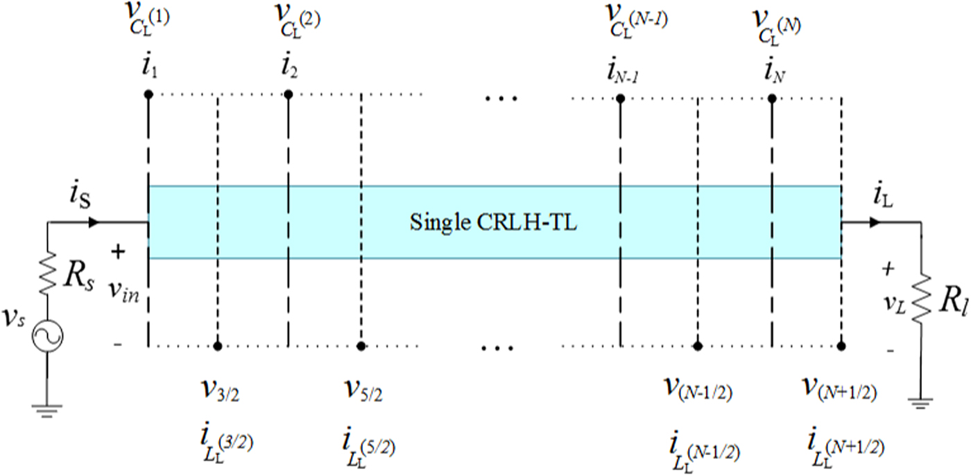
Fig. 3. Discretization of a single-conductor CRLH TL driven by a voltage source.
Boundary conditions
Boundary condition (BC) is first introduced in the same way as a single-conductor TL and then generalized to a MCTL. As demonstrated in Fig. 3, v in, v L, i s, and i L correspond to the voltages and currents at line input and load, respectively. By selecting the first equation in (7), BC is imposed at load for k = (N – 1/2) leading to [Reference Asadi and Honarbakhsh40]:
 $$L_R\lpar {i_N^{n + 1} -i_N^n} \rpar + \displaystyle{{\Delta t} \over 2}R\lpar {i_N^{n + 1} + i_N^n} \rpar + \displaystyle{r \over 2}\lpar {v_{N + 1/2}^{{\kern 1pt} n + 1} -v_{N-1/2}^{{\kern 1pt} n + 1}} \rpar + \displaystyle{r \over 2}\lpar {v_{N + 1/2}^{{\kern 1pt} n} -v_{N-1/2}^{{\kern 1pt} n}} \rpar + \displaystyle{r \over 2}\lpar {v_{C_L{\kern 1pt}}{_N^{n + 1}} + v_{C_L{\kern 1pt}}{_N^n} \rpar = 0,}$$
by replacing v L = R Li L and accordingly v N = R Li N−1, after a simple rearrangement, the above equation becomes:
 $$\left[ {-\displaystyle{r \over 2}v_{N-1} + \displaystyle{r \over 2}{(v_{C_L})}_N + \left( {L_R + \displaystyle{{\Delta t} \over 2}R + \displaystyle{r \over 2}R_L} \right)i_N} \right]^{(n + 1)} = \left[ { + \displaystyle{r \over 2}v_{N-1}-\displaystyle{r \over 2}{(v_{C_L})}_N + \left( {L_R-\displaystyle{{\Delta t} \over 2}R-\displaystyle{r \over 2}R_L} \right)i_N} \right]^{(n)},$$
where subscripts are associated with the array indices.
Similarly, the first equation in (7) for k = 1 at source, leads to:
 $$L_R\lpar {i_{3/2}^{n + 1} -i_{3/2}^n} \rpar \displaystyle{{\Delta t} \over 2}R\lpar {i_{3/2}^{n + 1} + i_{3/2}^n} \rpar + \displaystyle{r \over 2}\lpar {v_2^{n + 1} -v_1^{n + 1}} \rpar + \displaystyle{r \over 2}\lpar {v_2^n -v_1^n} \rpar + \displaystyle{r \over 2}\lpar {v_{C_L{\kern 1pt}}{_{3/2}^{n + 1}} + v_{C_L{\kern 1pt}}{_{3/2}^n}} \rpar = 0,$$
for − v S + R Si S + v in = 0 and replacing v in by v 1 and i S by i 1, becomes:
 $$\left[ {\displaystyle{r \over 2}v_2 + \displaystyle{r \over 2}{(v_{C_L})}_1 + \left( {L_R + \displaystyle{{\Delta t} \over 2}R + \displaystyle{r \over 2}R_S} \right)i_1} \right]^{(n + 1)}\cong {\kern 1pt} {\kern 1pt} \left[ {-\displaystyle{r \over 2}v_2-\displaystyle{r \over 2}{(v_{C_L})}_1 + \left( {L_R-\displaystyle{{\Delta t} \over 2}R-\displaystyle{r \over 2}R_S} \right)i_1} \right]^{(n)} + rv_S^n. $$
To generalize the corresponding BCs to a coupled-line coupler, let the first and second lines be, respectively, terminated by R S(1) and R S(2) at the source and by R L(1) and R L(2) at the load. Thus, RS and RL matrices defining the source and load impedance matrices, respectively, are:
 $$\left\{ \matrix{{\bf R}_S = diag\lpar {R_S^{{\kern 1pt} (1)}, \;R_S^{{\kern 1pt} (2)}} \rpar \hfill \cr {\bf R}_L = diag\lpar {R_L^{{\kern 1pt} (1)}, \;R_L^{{\kern 1pt} (2)}} \rpar \hfill} \right..$$
Terminal BCs are imposed to the aforementioned coupler by modifying NL and NR. BCs applied at load lead to:
 $$\left\{ \matrix{{\bf N}_L(2N-3:2N-2,:) = 0 \hfill \cr {\bf N}_L(2N-3:2N-2,2N-3:2N-2) = -\left( {\displaystyle{r \over 2}} \right){\bf I}_2 \hfill \cr {\bf N}_L(2N-3:2N-2,\,4N-1:4N) = {\bf L}_R + \left( {\displaystyle{{\Delta t} \over 2}} \right){\bf R} + \left( {\displaystyle{r \over 2}} \right){\bf R}_L \hfill \cr {\bf N}_L(2N-3:2N-2,\,6N-1:6N) = \left( {\displaystyle{r \over 2}} \right){\bf I}_2 \hfill \cr {\bf N}_R(2N-3:2N-2,:) = 0 \hfill \cr {\bf N}_R(2N-3:2N-2,2N-3:2N-2) = \left( {\displaystyle{r \over 2}} \right){\bf I}_2 \hfill \cr {\bf N}_R(2N-3:2N-2,\,4N-1:4N) = {\bf L}_R-\left( {\displaystyle{{\Delta t} \over 2}} \right){\bf R}-\left( {\displaystyle{r \over 2}} \right){\bf R}_L \hfill \cr {\bf N}_R(2N-3:2N-2,\,6N-1:6N) = -\left( {\displaystyle{r \over 2}} \right){\bf I}_2 \hfill} \right.$$
and the corresponding matrices for the source must be modified as follows:
 $$\left\{ \matrix{{\bf N}_L(1:2,:) = 0 \hfill \cr {\bf N}_L(1:2,3:4) = \left( {\displaystyle{r \over 2}} \right){\bf I}_2 \hfill \cr {\bf N}_L(1:2,\,2N + 1:2N + 2) = {\bf L}_R + \left( {\displaystyle{{\Delta t} \over 2}} \right){\bf R} + \left( {\displaystyle{r \over 2}} \right){\bf R}_S \hfill \cr {\bf N}_L(1:2,\,4N + 1:4N + 2) = \left( {\displaystyle{r \over 2}} \right){\bf I}_2 \hfill \cr {\bf N}_R(1:2,:) = 0 \hfill \cr {\bf N}_R(1:2,3:4) = -\left( {\displaystyle{r \over 2}} \right){\bf I}_2 \hfill \cr {\bf N}_R(1:2,\,2N + 1:2N + 2) = {\bf L}_R-\left( {\displaystyle{{\Delta t} \over 2}} \right){\bf R}-\left( {\displaystyle{r \over 2}} \right){\bf R}_S \hfill \cr {\bf N}_R(1:2,\,4N + 1:4N + 2) = -\left( {\displaystyle{r \over 2}} \right){\bf I}_2 \hfill} \right.$$
Finally, the time marching is conducted as:
 $${\bf N}_L{\bf U}^{n + 1} = {\bf N}_R{\bf U}^n + r{\bf V}_S^n, $$
where the  ${\bf V}_{\,S}^{\,n} $ is the input voltage vector at the nth time step.
Stability analysis
To ensure the stability issue of the CN-FDTD method, the associated amplification matrix  $\lpar {{\bf Q} = {\bf N}_L^{-1} \,{\bf N}_R} \rpar {\kern 1pt} $ and the corresponding Eigen-equation
  $\lpar {{\bf N}_R{\kern 1pt} {\bf u} = \lambda {\kern 1pt} {\bf N}_L{\kern 1pt} {\bf u}} \rpar $, are derived when Δt approaches infinity [Reference Asadi and Honarbakhsh40]:
 $$\eqalign{& \lambda \left[ {\matrix{ {\displaystyle{1 \over {2\Delta x}}\lpar {{\bf I}_N^ + -{\bf I}_N} \rpar \otimes {\bf I}_2} & {{\bf I}_N\otimes \left( {\displaystyle{{\bf R} \over 2}} \right)} & {\left( {\displaystyle{1 \over {2\Delta x}}} \right){\bf I}_N\otimes {\bf I}_2} & {{\bf I}_N\otimes 0_{2{\kern 1pt} \times {\kern 1pt} 2}} \cr {{\bf I}_N\otimes 0_{2{\kern 1pt} \times {\kern 1pt} 2}} & {\left( {\displaystyle{1 \over 2}} \right){\bf I}_N\otimes {\bf I}_2} & {{\bf I}_N\otimes 0_{2 \times 2}} & {{\bf I}_N\otimes 0_{2{\kern 1pt} \times {\kern 1pt} 2}} \cr {{\bf I}_N\otimes \left( {\displaystyle{{\bf G} \over 2}} \right)} & {\displaystyle{1 \over {2\Delta x}}\lpar {{\bf I}_N-{\bf I}_N^-} \rpar \otimes {\bf I}_2} & {{\bf I}_N\otimes 0_{2{\kern 1pt} \times {\kern 1pt} 2}} & {\left( {\displaystyle{1 \over {2\Delta x}}} \right){\bf I}_N\otimes {\bf I}_2} \cr {\left( {\displaystyle{1 \over 2}} \right){\bf I}_N\otimes {\bf I}_2} & {{\bf I}_N\otimes 0_{2{\kern 1pt} \times {\kern 1pt} 2}} & {{\bf I}_N\otimes 0_{2{\kern 1pt} \times {\kern 1pt} 2}} & {{\bf I}_N\otimes 0_{2 \times 2}} \cr}} \right]{\bf u} \cr & = \left[ {\matrix{ {\displaystyle{1 \over {2\Delta x}}\lpar {{\bf I}_N-{\bf I}_N^ +} \rpar \otimes {\bf I}_2} & {{\bf I}_N\otimes \left( {-\displaystyle{{\bf R} \over 2}} \right)} & {\left( {\displaystyle{{-1} \over {2\Delta x}}} \right){\bf I}_N\otimes {\bf I}_2} & {{\bf I}_N\otimes 0_{2{\kern 1pt} \times {\kern 1pt} 2}} \cr {{\bf I}_N\otimes 0_{2{\kern 1pt} \times {\kern 1pt} 2}} & {\left( {\displaystyle{{-1} \over 2}} \right){\bf I}_N\otimes {\bf I}_2} & {{\bf I}_N\otimes 0_{2 \times 2}} & {{\bf I}_N\otimes 0_{2{\kern 1pt} \times {\kern 1pt} 2}} \cr {{\bf I}_N\otimes \left( {-\displaystyle{{\bf G} \over 2}} \right)} & {\displaystyle{1 \over {2\Delta x}}\lpar {{\bf I}_N^- -{\bf I}_N} \rpar \otimes {\bf I}_2} & {{\bf I}_N\otimes 0_{2{\kern 1pt} \times {\kern 1pt} 2}} & {\left( {\displaystyle{{-1} \over {2\Delta x}}} \right){\bf I}_N\otimes {\bf I}_2} \cr {\left( {\displaystyle{{-1} \over 2}} \right){\bf I}_N\otimes {\bf I}_2} & {{\bf I}_N\otimes 0_{2{\kern 1pt} \times {\kern 1pt} 2}} & {{\bf I}_N\otimes 0_{2{\kern 1pt} \times {\kern 1pt} 2}} & {{\bf I}_N\otimes 0_{2 \times 2}} \cr}} \right]{\bf u},} $$
and as Δt→∞, it finally further simplifies to:
 $$(1 + \lambda )\;{\bf u} = 0,$$
which satisfies the unit spectral radius, i.e., the unconditional stability of the CN-FDTD method is warranted [Reference Honarbakhsh and Asadi29]. The stability results are numerically validated later for the specific fabricated coupler.
Extraction of the unit-cell parameters
In order to extract unit-cell parameters, first the scattering parameters of the corresponding series capacitance and shunt inductance structures are computed separately by either full-wave analysis or measurements. Then the S-parameters are converted to the corresponding Z-parameters or Y-parameters [Reference Pozar14]. Finally, the LC parameters are retrieved according to standard derivations with respect to the extraction frequency [Reference Kantartzis and Tsiboukis41]. According to Fig. 1, this CRLH coupler, fabricated on the Rogers RT/Duroid 5880 substrate with dielectric constant ε r = 2.2 and thickness of h = 1.27 mm, contains nine unit cells with each having a length of 6.1 mm, assumed to be lossless (R (1) = R (2) = G (1) = G (2) = 0). The extracted lumped circuit parameters of each unit cell are reported in Table 1.
Table 1. Extracted values of the CRLH coupled-line unit cell [Reference Caloz and Itoh42]
Results and discussion
Accuracy
In this section, the accuracy of the CN-FDTD method applied to the CRLH coupled-line coupler is investigated and compared with the LF-FDTD method. A sinusoidal excitation oscillating at 3.9 GHz is connected to the input port and the outputs are measured from the through and the coupled ports of the coupler.
As mentioned before, there is a trade-off between CPU time and accuracy of the CN-FDTD method. Here, for 10 × Δt max (Δt max = 1.8 ps which is the maximum time step size corresponding to the LF scheme), the accuracy is well maintained, and by increasing the time step size, the accuracy is degraded as shown in Fig. 4.
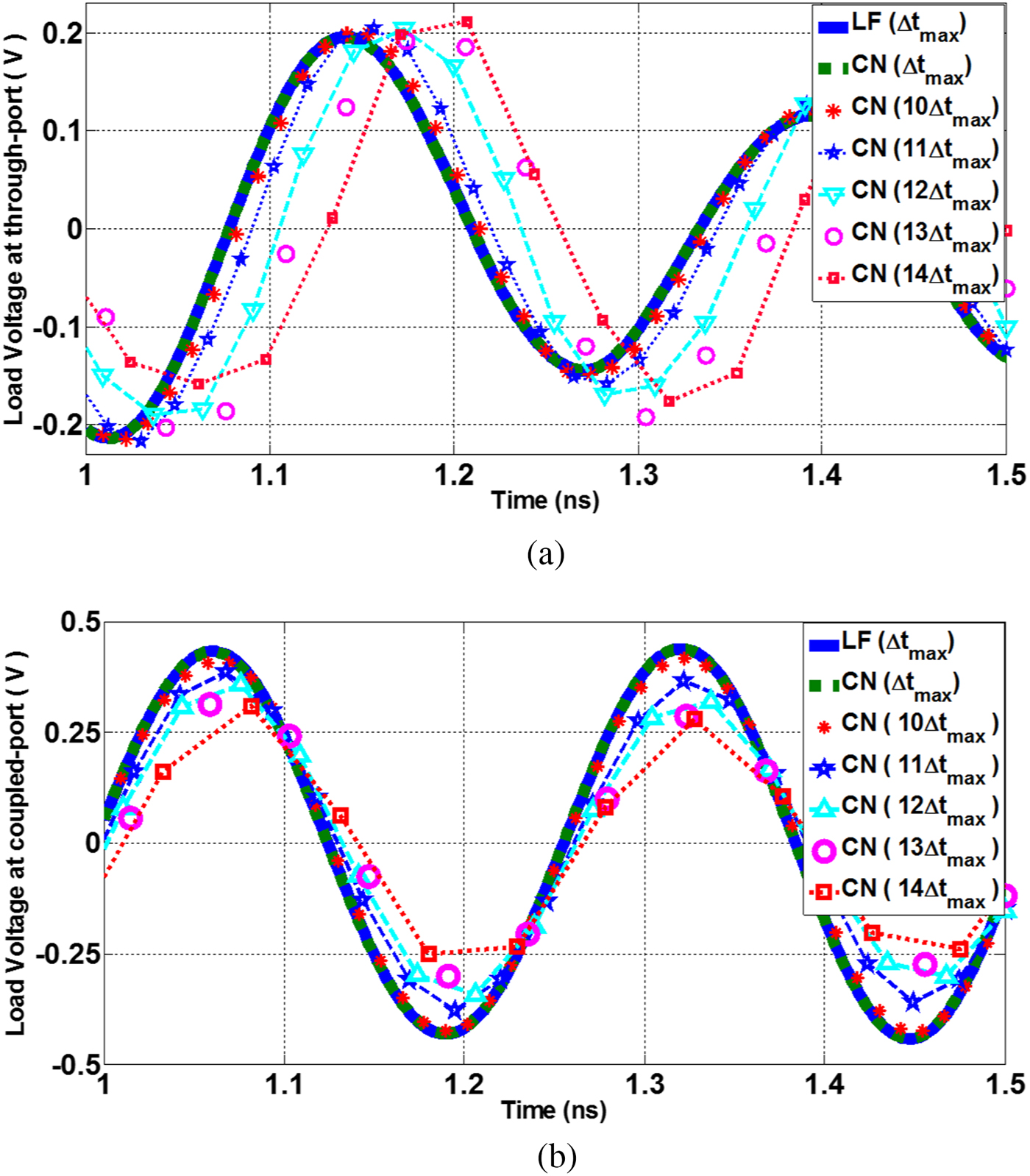
Fig. 4. The voltage at the end of (a) through port, (b) coupled port corresponding to the LF at Δt max and CN at Δt max and the CN at k × Δt max (k varies from 10 to 14).
In order to mathematically assess this dependency between the computation cost and accuracy, the relative error (denoted by r e) computed by the CN and LF schemes is reported in Table 2, wherein:
 $$r_e = \displaystyle{{\sqrt {\sum\nolimits_i {{\vert {V_o^{\Delta t} \,(i{\kern 1pt} \Delta t)-V_o^{\Delta t_{{\kern 1pt} \max}} \,(i{\kern 1pt} \Delta t)} \vert } ^2}}} \over {\sqrt {\sum\nolimits_i {{\vert {V_o^{\Delta t_{{\kern 1pt} \max}} \,(i{\kern 1pt} \Delta t)} \vert } ^2}}}}, $$
where  $V_o^{{\kern 1pt} \Delta t_{{\kern 1pt} \max}} $ and
  $V_o^{\Delta t} $ represent load voltages at the end of either through or coupled ports for Δt max and Δt voltage values, respectively [Reference Gholami Mayani and Asadi43].
Table 2. Estimated error (r e) versus Δt

According to Table 2, the time step size of 10Δt max is considered to be the threshold of optimum accuracy with a negligible error value, and that beyond this point, the response becomes erroneous noticeably. Therefore, a clear trade-off is observed between CPU time and desired accuracy.
Time gain
The time gain, as the relative CPU time of the LF-FDTD compared with the CN-FDTD method (T LF/T CN), versus different temporal step size at 3.9 and 6 GHz is reported in Table 3.
Table 3. Time gain of the CN method for different time step sizes

As it is evident, the CN method requires much less CPU time compared with the LF method as no constraint is imposed on temporal step size until the accuracy level is satisfied. In this study, for Δt = 10Δt max, the time gain accompanied to a satisfactory accuracy is achieved.
Stability
To examine the stability, the spectral radius of the amplification matrix for the LF- and CN-FDTD methods is computed for a range of Δt and reported in Fig. 5. In the LF scheme restrained by the CFL number, the spectral radius rises unboundedly once Δt becomes greater than Δt max = 1.8 ps at 3.9 GHz. Thus, the LF method becomes unstable, though the spectral radius of the CN method is equal to unity.
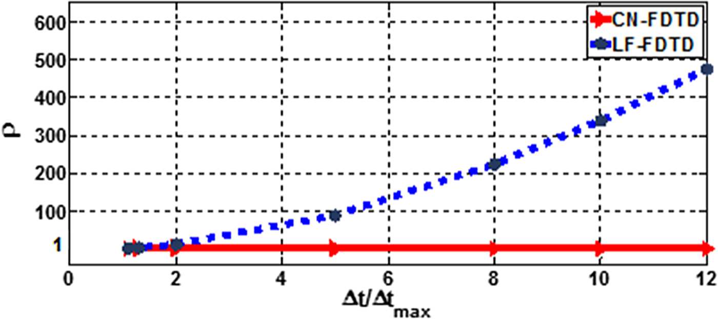
Fig. 5. The spectral radius analysis versus time step size.
Scattering parameters
The scattering parameters (S-parameters) can be extracted from the time-domain results [Reference Asadi and Honarbakhsh40]. It is conducted by first computing the corresponding Z-parameters according to:
 $$Z_{ij}(\,f) = \left. {\left[ {\displaystyle{{V_i(\,f)} \over {I_j\lpar f \rpar }}} \right]} \right \vert _{I_k = 0,\;k\ne j},$$
where subscripts i and j stand for the port numbers. In this approach, Z ii and Z ji are computed by applying a proper Gaussian excitation pulse to the beginning of the port i, while port j is open-circuited. Similarly, Z ij and Z jj are extracted by applying the excitation signal to port j and open-circuiting port i. Then the S-parameters are retrieved as [Reference Pozar14]:
 $${\bf S} = \lpar {{\bf Z} + Z_0{\bf {\rm I}}} \rpar ^{-1}\lpar {{\bf Z}-Z_0{\bf {\rm I}}} \rpar .$$
The coupled-line coupler as a four-port device is excited by a Gaussian pulse with peak time and spread of 80 and 20 ps, respectively, at the input port and the outputs are extracted from the through and coupled ports while matched to Z 0 (50 Ω resistor). There is a backward-wave coupling from approximately 3.2–4.5 GHz and also the through coupling ranging from 1.5 to 3.1 GHz, showing a dual-band operation. As illustrated in Fig. 6, the S-parameter results extracted from both LF- and CN-FDTD methods are in good agreement with the measurement results.

Fig. 6. S-parameters of the CRLH coupled-line coupler shown in Fig. 1. (a) Magnitude and (b) phase.
Conclusion
In this paper, the CN-FDTD was successfully used to analyze a CRLH coupled-line coupler. Unconditional stability of this method has been confirmed. The accuracy of the CN has been verified by comparison of the results from CN to LF scheme and also the measurements. It is concluded that the CN-FDTD method has improved the time gain with satisfying accuracy level, whilst the temporal step size increased up to 10 times.
Author ORCIDs
Mahdieh Gholami Mayani http://orcid.org/0000-0002-4301-5734.
 Mahdieh Gholami Mayani was born in Iran, in 1985. She received her B.S. from Shahrood University of Technology and M.S. degree in electrical engineering from Shahid Beheshti University of Tehran, respectively, in 2007 and 2016. She is currently research assistant in the Department of Electrical Engineering at the Shahid Beheshti University. Her research interests are numerical electromagnetics, Metamaterials, passive and active devices and multiconductor transmission lines.
 Shahrooz Asadi received the B.Sc. degree in Electrical Engineering and the M.Sc. degree in Electronics both from Amirkabir University of Technology (Tehran Polytechnic), in 2003 and 2007, respectively and the Ph.D. degree in Electronics in the School of Information Technology and Engineering (SITE), University of Ottawa, Ottawa, ON, Canada. He joined Shahid Beheshti University in 2011 where he is an assistant professor. His research interests include linear and nonlinear time-domain modeling of millimeter-wave transistors, RF design of active and passive devices, design and optimization of solid state devices and multiconductor transmission lines and printed circuit board.
 Dr Shokrollah Karimian is an Assistant Professor in School of Electrical Engineering at Shahid Beheshti University. As a member of IEEE, with over 50 publications, he has made valuable contribution to the RF and microwave/mm-wave community.