


Introduction
The design of integrated circuits requires knowledge of the materials properties for the substrate that is also used in designing a proper radiating element and feeding structure that use monolithic microwave integrated circuits like coplanar strips and coplanar waveguide (CPW). For many applications, the information about design parameters could be retrieved from the dielectric material measurement. In addition, knowing the dielectric permittivity can provide the designer preliminary information about the required dimensions of microwave elements. The permittivity estimation of multilayer dielectric plate could be realized by means of the wall-thru radar: [Reference Kobayashi, Takaoka, Kawamura, Cui and Yamaguchi1]. Another way of the extraction of the complex permittivity is to use multi-layered conductor-backed CPW as a sensor for non-destructive electromagnetic measurement calculation: [Reference Kang, Cho, Cheon and Kwon2]. More recent applications in the area of aerospace, automotive, food and medical industries have also been found to benefit from the knowledge of the dielectric properties: [3].
Computer-aided design (CAD) software could be used to estimate the dimensions of the microwave element, these programs are expensive, need licensing and require high computing facilities. The simulation accuracy of electromagnetic problems is reduced as material dispersion becomes more significant with increasing frequency: [Reference Seiler, Klein and Plettemeir4].
The mathematical formulation can be used to obtain the effective permittivity of multilayer medium, a non-node-based, third-order finite element method (FEM) formulation is suggested for the calculation of effective permittivity of transmission lines (TLs) with a rectangular cross-section and multilayered isotropic dielectric: [Reference Petrović and Mančić5]. Permittivity and permeability measurements are required in numerous applications for a large variety of materials. The most widely used techniques in the microwave region are cavity resonators, free space, open-ended coaxial probe, and TLs [Reference Boughriet, Legrand and Chapoton6]. This is also required for the increased multilayer fabrication and radiofrequency (RF) characterization of a high-density stacked metal-insulator-metal capacitor: [Reference Tseng and Xie7].
In the RF band, printed antennas are popular due to their compactness in a defined area, low cost of production, negligible volume, and reproducibility. Analysis of printed antennas requires the knowledge of the substrate characteristics and the calculation of Sommerfeld's integrals, which are especially difficult to solve when the source and the field points are on the same substrate: [Reference Parhami, Rahmat-Samii and Mittra8]. To reduce the size of antenna, various techniques have been documented. Multilayer substrate can be used to reduce the size of the compact planar inverted-F antenna (PIFA) when used with electromagnetic bandgap structure for surface area radar reduction in mobile application: [Reference Kwak, Sim, Kwon and Yun9]. The other simplest method to reduce the size of antennas is to use a high dielectric constant for a given frequency: [Reference Balanis10]. The substrate thickness is chosen to be smaller than the wavelength in order to reduce the fundamental modes of transverse-magnetic surface wave (TM 0): [Reference Rana and Alexopoulos11].
The paper is organized in the following way: In the section ‘Effect of substrate on antenna design’, we elaborate the approach used to relate the antenna dimension to the effective permittivity. In the section ‘Determination of the effective permittivity by ratio of resonance method’, we introduce the ratio of resonance method to extract the effective permittivity of a substrate by varying the relative permittivity and the height of the substrate. At the end of this section, we propose an analytic expression of the effective permittivity that is related to the relative permittivity and the height of the substrate. The section ‘Evaluation of the effective permittivity of multilayer substrate’ shows an application of the analytic expression for a multilayer substrate. The work and the future recommendations are concluded in the section ‘Conclusion’.
Effect of substrate on antenna design
We have considered the case of the dipole antenna to extract the effective permittivity. Other methods could be used like multilayer CPW structure: [Reference Kang, Cho, Cheon and Kwon2], wall-thru radar image: [Reference Kobayashi, Takaoka, Kawamura, Cui and Yamaguchi1], or using TL with multilayered medium and weak FEM formulation: [Reference Petrović and Mančić5].
An example of the dipole of length d printed on a substrate of permittivity ɛr and a height h is shown in Fig. 1.

Fig. 1. Example of dipole printed on substrate.
From the above, the dimensions of the antenna will be affected by the relative permittivity. For a dipole antenna, two types of resonance are present, the first resonance “series” and the second resonance “parallel (anti resonance)”: [Reference Balanis10]:
• For the series resonance, the imaginary part of the input impedance for the antenna is zero and its real part is weak: [Reference Kogure, Kogure and Rautio12]. The length of the antenna at the series resonance in the air will therefore be: [Reference Balanis10]:
(1)$$d_{series} = 0.48{\rm \ast }\lambda.$$
• For the parallel resonance, the imaginary part of the input impedance for the antenna is zero and its real part is high: [Reference Kogure, Kogure and Rautio12]. The length of the antenna at resonance parallel in the air will therefore be: [Reference Balanis10]:
(2)$$d_{\,parallel} = 0.96\ast \lambda \quad \;{\rm Where}\,\,\lambda = c/f$$


where d is the dipole length at series and parallel resonance, λ is the wavelength, f is the operating frequency, and c is the speed of light in the vacuum.
Subsequently, the dipole length at parallel resonance is identified, which we will use to extract the effective permittivity. Equation (1) and (2) are valid in the case where the medium surrounding the antenna is air. In the presence of several environments, the notion of the effective permittivity is introduced; this notion is illustrated in Fig. 2 where multilayer substrates of different relative permittivity are equivalent to one substrate with effective permittivity. Note that we are considering the parallel resonance. Our final objective ultimately is to determine the resonance frequency not the current at the resonance frequency. In addition, since we know that, parallel resonance is a function of two factors: the feed location and the antenna geometry: [Reference Obeidat, Raines and Rojas13], we are considering the dipole with a feeding location at the center of the dipole arms only to have an initial estimation of the effective permittivity.

Fig. 2. Concept of the effective permittivity.
Note that a non-magnetic substrate is considered and thus the relative permeability is considered to be equal to one. Equation (3) is valid for the nonmagnetic substrate: [Reference Rialet, Sharaiha, Tarot and Delaveaud14]. The dipole length will then become

ɛreff is the effective permittivity of the substrate.
The extraction of the effective permittivity of the substrate, with a given material and on which an antenna is printed, is presented. The “Ratio of resonance method” is based on the frequency of resonance ratio of the antenna printed on a substrate and in the air. An empirical equation is presented to calculate the effective permittivity that will be presented as a function of the relative permittivity, substrate thickness, and the length of the antenna in air.
The procedure used to extract the effective permittivity of the substrate is shown in Fig. 3.
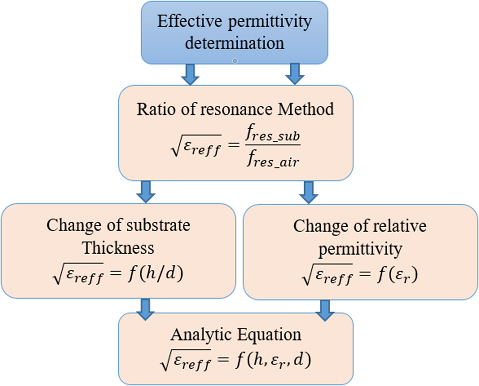
Fig. 3. Procedure for extracting the effective permittivity.
Determination of the effective permittivity by ratio of resonance method
This section describes how the effective permittivity is extracted using the ratio of the resonance method, which helps in determining the substrate effective permittivity by referring to the relative permittivity.
The procedure is as follows:
• Determine the resonance frequency $f_{res \hbox{-} sub}$
(parallel in our case) of printed dipole having a length d on a substrate with a given permittivity.• For the same antenna dimension d, determine the resonance frequency in the case of air $f_{res \hbox{-} air}$
.• The effective permittivity will therefore be the ratio of the resonance frequency for a dipole printed on substrate and on air
(4)$$\sqrt {\varepsilon _{reff}} = f_{res \hbox{-} sub}/f_{res \hbox{-} air}. $$


Variation of the relative permittivity
In this part, the analytical approach is detailed. According to the ratio of resonance method, the electromagnetic simulations, carried out by CST Microwave Studio (CST MWS), one of the 3D CAD software used in our case [Reference Barakat J Moussa15], aim to determine the effective permittivity with respect to the relative permittivity for a given thickness of the substrate.
Based on the permittivity graphs, a setup of a model structure for the trend curves linking the effective permittivity ɛreff and the relative permittivity ɛr is proposed.
The trend curves of the ɛreff with respect to ɛr are illustrated in Fig. 4. The variation of the square root of the effective permittivity $\sqrt {\varepsilon _{reff}}$ is a power function with respect to relative permittivity ɛr. The equivalent equation has the following form:


Fig. 4. Effective permittivity with respect to relative permittivity for different height of substrate.
From the obtained value of the effective permittivity, the objective is to acquire a regression model with a given adjustment function. From Fig. 4, the regression is a power function. In Table 1, we show the different coefficients a h and b h from equation (5). In each regression, the coefficient of determination R 2, which is a statistical measure of how close the data are to the fitted regression line, is shown. A value of 100% indicates that the model explains all the variability of the response data around its mean value. The value of R 2 is close to one which validates our assumption for the regression model.
Table 1. Power model coefficients for different substrate thickness.

Consequently, the a and b parameters are determined by taking the average of the coefficients a h and b h found from each curve in Fig. 4. Finally, the equation of regression of the effective permittivity is:

The standard deviation for the coefficients a h and b h is 3%, which allows us to say that this averaging is acceptable.
Variation of the substrate thickness
After finding the first equation of the effective permittivity with respect to the relative permittivity, the second step is to determine the regression of the effective permittivity with respect to the relative substrate thickness.
Electromagnetic simulations have been conducted using CST MWS: [Reference Barakat J Moussa15]. Based on the ratio of the resonance method, the regression of the effective permittivity with respect to the relative height of the substrate is studied. Thus, the trend curves of $\sqrt {\varepsilon _{reff}}$ with respect to the relative height of the substrate h/d for different relative permittivity ɛr have been plotted Fig. 5. The dielectric permittivity could be modelled as quadratic polynomial [Reference Tendeku and Misra16, Reference Ghalichechian and Sertel17]. In addition, the trend curves show a quadratic regression, hence the goal is determining the coefficients of the variation $\sqrt {\varepsilon _{reff}}$
 with respect to the relative height h/d. Note that a dipole of a fixed length has been used. In addition, the extraction of the effective permittivity is achieved by using the concept of equation (4)

Fig. 5. Effective permittivity with respect to relative height for different relative permittivity.
Finally, the form of the quadratic regression will have the following polynomial equation:

Following the same regression approach, the coefficients a e, b e, c e, are determined from the trend curves relating the effective permittivity and the relative height.
As per Table 2, the majority of the coefficient of determination R 2 is close to one, which shows that this quadratic regression is close to the studied data.
Table 2. Coefficients of the regression for different permittivity.

The next step is to introduce the notion of permittivity into these equations. According to equations (6) and (7), a new form of the quadratic equation is offered by introducing the function of relative permittivity. The coefficients a e, b e, c e from Table 2, are divided by 1.222*(ɛr)0.53 for each value of permittivity to obtain the values of a es, b es, c es in Table 3.
Table 3. Coefficients of the regression for different permittivity.

Finally, the averaging of the coefficients a es, b es, c es is done to get the final coefficients. Table 4 presents the mean and standard deviation of these coefficients.
Table 4. Mean and standard deviation for the coefficients.

The final equation of the effective permittivity with respect to the relative permittivity and the relative height which is the dipole length in the air over the substrate thickness is:

Numerical validation
After the determination of equation (8) linking the permittivity and the relative height, it is convenient to compare the values of the effective permittivity using the analytical equation and the values obtained by electromagnetic simulation.
Figure 6 shows the difference between the values obtained from electromagnetic simulation extracted from CST and the analytic values from equation (8). As shown in the graphs, for different values of relative permittivity, the relative error is in the 5–10% range except for ɛr = 2 where it is 14% at a relative height h/d = 0.1. The idea is to have a preliminary estimation of the effective permittivity that helps the designer. The designer should start with these values and confirm by electromagnetic simulation of the final design of the antenna for example. In order to validate our design, we have compared our analytic model to the one presented in [Reference Rialet, Sharaiha, Tarot and Delaveaud14], for a dipole operating at 6 GHz printed on a substrate of height h = 350 μm, and with relative permittivity ɛr = 6, the effective permittivity in our case is 3.55 with respect to 3.5 from the analytic model of [Reference Rialet, Sharaiha, Tarot and Delaveaud14].

Fig. 6. Numerical validation of the effective permittivity.
Evaluation of the effective permittivity of multilayer substrate
For the estimation of the integrated dipole length on a multilayer substrate, the value of the effective permittivity of this substrate should be known. In the preceding parts, a method to determine the effective permittivity of a substrate with a single layer is presented. The next step is to take advantage of these estimates to determine the effective permittivity of a multilayer substrate like silicon on insulator (SOI).
The procedure to follow is described in Fig. 7. The goal is to determine a layer with an equivalent permittivity and equivalent height and use the proposed analytic expression to determine the effective permittivity of the substrate. We are considering the case of a multilayer substrate in this study.

Fig. 7. Equivalent relative permittivity concept of a multilayer substrate.
Variation of the relative permittivity
Different expressions, describing the equivalent substrate model of multilayer structure, exist in the literature, among which two could be stated: expression developed by Lee et al.: [Reference Lee, Ho and Dahele18] and Krasweski [Reference Kraszewski19]
The expression developed by Krasweski: [Reference Kraszewski19] is (Fig. 8):

where v i is the fractional volume of the layer i and where ɛh and ɛi are the relative permittivity of the host medium and inclusions. This equation is symmetrical and does not involve the form of structures contrary to many formulas in the literature: [Reference Pavageau20] that is why it is used to determine the equivalent permittivity: [Reference Fu, Vuong, Dussopt and Ndagijimana21].

Fig. 8. Krasweski model.
The fractional volume of the layer i is calculated by dividing the volume of the layer i over the total volume, where s is the substrate surface

Expression of the equivalent permittivity
Subsequently, this expression is used to determine the parameters ɛmulti and h eq of the equivalent SOI substrate. This preliminary study could help the designer to start the design. Other parameters could be added when doing the design using the 3D CAD software in order to have the effect of the substrate.
From the information about the substrate, we have used Krasweski model (equations (9) and (10)) to get equivalent parameters of the equivalent substrate presented in Table 5.
Table 5. Equivalent height and relative permittivity of SOI substrate.

According to Table 5, the equivalent relative permittivity of the SOI substrate is 11.71, with an equivalent height of 357.51 μm.
By applying equation (8), the effective permittivity of the SOI substrate can be determined. Thus, the value of effective permittivity is$\;\sqrt {\varepsilon _{reff}} = 2.516$ , (ɛreff = 6.33). Bunea et al. [Reference Bunea, Neculoiu and Muller22] have also developed an analytic equation for the effective permittivity using CPW and has considered a high resistive silicon substrate, the analytic result (ɛreff = 6.30) is comparable to our obtained values. This study is a step towards the determination of the effective permittivity for dipole antennas integrated on SOI substrate. An estimate of the length of a dipole antenna, operating at 60 GHz and an application of equations (1) and (3) gives us an antenna of length 937 μm. The obtained results were the basis of other design of antenna on high SOI substrate: [Reference Fu, Vuong, Dussopt and Ndagijimana21, Reference Barakat, Delaveaud and Ndagijimana23, Reference Barakat, Delaveaud and Ndagijimana24]. The layers near the antenna are electromagnetically more influential on the parameters of the antenna, but their dimensions are very small compared to the silicon layer, leading to a limited influence on the equivalent relative permittivity.
We have used the same procedure for the design of a 60 GHz fully integrated dipole antenna, incorporating an interdigitated structure, and realized on 0.13 μm SOI process from STMicroelectronics, with the following parameters: substrate dimensions are 1200 *2400 μm2, dipole's length = 871 μm (Fig. 9) [Reference Barakat, Delaveaud and Ndagijimana23]. The difference in the size between the initial estimated length (937 μm) of the dipole and the realized one (871 μm) was in the order of 7%. These results have helped to reduce the optimization process when we have designed other antennas [Reference Fu, Vuong, Dussopt and Ndagijimana21,Reference Barakat, Delaveaud and Ndagijimana23,Reference Barakat, Delaveaud and Ndagijimana24].

Fig. 9. Schematic of the dipole with balun on SOI [Reference Barakat, Delaveaud and Ndagijimana23].
Conclusion
The determination of the effective permittivity is an essential step for the design of antennae and feeding structures. The main objective of this article was to propose a method for determining the effective permittivity of the multilayer substrate. Electromagnetic simulations have been conducted to study the effect of relative permittivity and substrate thickness on the resonance of the antenna, which provides trending curves that helped in obtaining the values of effective permittivity. In addition, an analytical model that helps the designer to evaluate the effective permittivity with respect to the relative height of the substrate has been proposed. The analytic equation was based on the study of the parallel resonance for the antenna, the future works will focus on using the series resonance to review and validate the analytic equation. The example of multilayer substrate like SOI substrate has been demonstrated to benefit from the real application of the proposed method.
 Julien Moussa H. Barakat was born in Yohmor, in 1981. He received the Bachelor of Engineering degree from the Beirut Arab University, Lebanon in 2003 and the M.Sc. degree in Microwave and optical communication from the University of Paul Sabatier, France in 2004. He achieved his Ph.D. degree in the LETI in the French atomic energy commission (CEA) and the IMEP/INPG/Minatec, Grenoble, France. Currently, he is an Assistant professor in the College of Engineering and Technology, American University of the Middle East (AUM), Kuwait. His research interest includes antenna and microwave elements design, high impedance surface, SOI integrated millimeter antenna, measurement techniques, permittivity, RF elements for IOT, optical transmission, and development of optical elements.
 Fabien Ndagijimana received the Ph.D. degree in microwave and optoelectronics from the Institut National Polytechnique de Grenoble (INPG), France, in December 1990. In December 1990, he then joined the Faculty of Electrical Engineering ENSERG as an Associate Professor, where he teaches microwave techniques and electromagnetic modeling. Since September 1997, he joined the Université Grenoble Alpes, where he is currently a Full Professor with the Institut Universitaire de Technologie (IUT). He is currently a Professor with Université Grenoble Alpes, Grenoble, France. His research activity focuses on the characterization and electromagnetic modeling of microwave devices for wireless applications, signal integrity in high-speed applications, and test tools for electromagnetic compatibility standards.


