


I. INTRODUCTION
Antenna pattern measurement forms a critical task in the testing and characterization of antennas. In general, the far-field [Reference Yamaguchi, Kimura, Komiya and Keizo1] and near-field [Reference Yaghjian2] approaches are used to measure antenna patterns. Far-field measurement is commonly used because it is the most direct way to obtain an antenna pattern. However, according to the definition of the far-field [Reference Elliott3], the distance between the receive antenna and the antenna under test (AUT) should be greater than 2D2/λ, where D denotes the maximum size of the antenna and λ denote the wavelength. If the size of the antenna is considerably larger than the wavelength, the space required to perform the far-field antenna measurement is large. On the contrary, in the near-field approach, when the E-field in the near-field region is measured, there is no requirement of a large space to satisfy the far-field condition. Therefore, near-field measurement is practically useful for large-sized-antenna measurement.
The near-field antenna measurement system comprises a scanning plane, a received antenna, and an AUT. If the scanning plane is planar, the E-fields emitted by the AUT on the scanning plane are measured by moving the received antenna along the horizontal (left to right) and vertical (upward and downward) directions in a step-by-step manner until the entire region in the scanning plane is covered. Using these measured E-fields, the antenna pattern can be reconstructed by the transformation from the near-field measured data to the far-field pattern [Reference Paris, Marshall Leach and Joy4]. To accurately obtain the measurement pattern, near-field antenna measurement requires measuring the E-fields of the AUT with a spectral spacing smaller than λ/2 as per the sampling theorem [Reference Paris, Marshall Leach and Joy4]. Therefore, using the near-field method to measure a large-size antenna is time-consuming because the scanning plane is usually considerably larger than the wavelength. Thus, a large number of data points are required. For example, in [Reference Tsai, Wu, Chen, Lee and Wang5], 2601 measurement points were required with a spectral spacing of 0.15 cm for measuring a 74-GHz horn antenna. If each point takes approximately 1 s to be measured, the total measuring time works out to about 43 min.
In this context, researchers have proposed certain methods to reduce the number of data measurements [Reference Giordanengo, Righero, Vipiana, Vecchi and Sabbadni6, Reference Qureshi, Schmidt and Eibert7]. In [Reference Giordanengo, Righero, Vipiana, Vecchi and Sabbadni6], a model builder was used to generate the near-field/far-field bases, and subsequently, these generated bases were utilized to match the measurement results. Although using this method can reduce the number of measurement points from 60 000 to 505 with the use of a simple model and from 60 000 to 205 with a complete model, the drawback is that a complete simulation model requires 15 h for its construction, and a complete basis requires the construction of 42 simulation models. In other words, this method may need more time to complete the measurement if the simulation time is taken into consideration. In [Reference Qureshi, Schmidt and Eibert7], the scanning plane is divided into m, m + 1, m + 2 … , m + n rings. Using the measured data in ring m, the extrapolated data for ring m + 2 is evaluated. If the differences between the extrapolated and measured data in ring m + 2 are large, the data in ring m + 1 is measured. Otherwise, the data of ring m + 1 need not be measured. Because certain data points are not measured, the number of measurements time reduces. Although this method can reduce the number of measuring points by 70.7%, the E-field information in the near-field requires to be known before commencing the measurement.
In [Reference Chiu, Tsai and Tsai8], a basic concept to accelerate the speed of the near-field antenna measurement is proposed. This is achieved by sparse E-field sampling in the region where the E-field changes smoothly and dense sampling in the region where the E-field changes rapidly. The use of the method proposed in this study can reduce the number of measuring points by ~69% while yielding a pattern similar to that obtained with the sampling theorem. Because an iterative approach is used, there is no requirement to determine the E-field information before measurement. Therefore, this measurement method is suitable to measure different kinds of antenna patterns.
It is noticeable that the complete measured data following the sampling theorem is used to verify the concept in [Reference Chiu, Tsai and Tsai8]. The result shows that a portion of data from the complete measured data is required to reconstruct the accurate pattern. However, it is necessary to provide a demonstration of measuring the antenna by using this acceleration concept. Thus, in this paper, a near-field system is built for the demonstration. The complete details of the method based on the concept of [Reference Chiu, Tsai and Tsai8] are presented. To verify the robustness of the proposed method, we examine a 15-GHz horn antenna with main beam angle θ = 10°. Our results show a 64.9% reduction in the number of measuring points, and we further verify the robustness of this method.
II. PROBLEM STATEMENT
In general, the antenna pattern can be perfectly reconstructed with the sampling theorem of λ/2. However, the use of this theorem typically requires a large number of measurement points; the E-field must be measured for every step of λ/2 in the scanning plane. For instance, the measurement of a 15-GHz horn antenna with aperture size of 15.5 × 13 cm2 along with the far-field antenna pattern in the range from −60° to 60° corresponds to scanning plane dimensions of 51 × 51 cm2 and a λ/2 spectral spacing of 1 cm. Thus, measuring the pattern of this horn antenna requires 2601 measurement points. If each point requires approximately 1 s of measurement time, the total measuring time of measuring this pattern is about 43 min.
To address this time-consuming problem, we propose a technique to accelerate the near-field antenna measurement. The acceleration is achieved by sparse E-field sampling in the region where the E-field changes smoothly and dense sampling in the region where the E-field changes rapidly. For example, Fig. 1 shows the measured near-field data of a 15-GHz horn antenna. The E-field changes smoothly in region A, and thus, sampling here is sparse. On the other hand, the E-field changes rapidly in region B, and thus, dense sampling is performed. Because large sections of the near-field exhibit smooth E-fields, the number of data points effectively reduces.

Fig. 1. Measured near-field data of a 15-GHz horn antenna.
Figure 2 shows the schematic of our proposed system along with the relevant parameters. We consider the position of the AUT to be the point of origin in this system. Parameters x, y, and z denote the coordinates of the received antenna, θ and ϕ denote the two components formed by the original point, x- and y-axes, respectively, and h denotes the distance between the received antenna and the AUT. Further, the rectangles bounded by the minimum x and y values (x min and y min ) and maximum x and y values (x max and y max ) represent the scanning plane of the received antenna. In the following discussion, we assume that the E-field is measured for a fixed h value. Although the E-field sampled at (x, y) varies with h, the reconstructed antenna pattern does not change because of the equivalence principle [Reference Chen9]. In this measurement, h is fixed to a value that is suitable to recover the antenna patterns.

Fig. 2. Schematic of proposed system with relevant parameters.
The transformation from the near-field measured data to the far-field pattern is obtained as below. Let P
B
(x, y) denote the E-field measured at (x, y) when for a suitable h. Further, let
 $E_\theta ^{AUT} $
and
$E_\theta ^{AUT} $
and
 $E_\phi ^{AUT} $
denote the θ and ϕ components, respectively, of far-field radiation patterns of the AUT, and
$E_\phi ^{AUT} $
denote the θ and ϕ components, respectively, of far-field radiation patterns of the AUT, and
 $E_\theta ^r $
and
$E_\theta ^r $
and
 $E_\phi ^r $
denote the θ and ϕ components, respectively, of the E-fields of the received antenna in far-field. According to the method described in [Reference Paris, Marshall Leach and Joy4],
$E_\phi ^r $
denote the θ and ϕ components, respectively, of the E-fields of the received antenna in far-field. According to the method described in [Reference Paris, Marshall Leach and Joy4],
 $E_\theta ^{AUT} $
and
$E_\theta ^{AUT} $
and
 $E_\phi ^{AUT} $
can be calculated using P
B
(x, y),
$E_\phi ^{AUT} $
can be calculated using P
B
(x, y),
 $E_\theta ^r $
, and
$E_\theta ^r $
, and
 $E_\phi ^r $
as follows:
$E_\phi ^r $
as follows:
 $$\eqalign{& E_\theta ^{AUT} (\theta ,\;\phi )E_\theta ^r (\theta , - \phi ) - E_\phi ^{AUT} (\theta ,\;\phi )E_\phi ^r (\theta , - \phi ) = \cr & \quad C\;\cos \theta {e^{jkh\cos \theta }} \times \int_{ - \infty }^\infty {\int_{ - \infty }^\infty {{P_B}} } (x,y){e^{jkx\sin \theta \cos \phi + jky\sin \theta \sin \phi }}dxdy.} $$
Here, C denotes a constant determined by ω and the free space wave number is denoted by k = 2π/λ.
III. PROPOSED METHOD
The concept underlying the proposed method is the determination of whether the interpolated data in a rectangular block formed by any four adjacent measured points in the scanning plane can accurately represent the measured data required to reconstruct the antenna pattern. If the data are sufficiently accurate, measuring additional points within the block is unnecessary.
The flowchart of the proposed method is shown in Fig. 3. The approach comprises an initialization and four steps. The initialization includes initial block selection, rectangular interpolation, and division of the initial block. Step 1 describes the procedure for block selection. In Step 2, the rectangular interpolation technique is used to approximate the data necessary for reconstructing the antenna pattern. Step 3 involves checking whether the interpolated data is sufficient for reconstruction. Step 4 provides the necessary information for the block selection in Step 1. These four steps are repeated until all the interpolated data can accurately represent the measured data required to reconstruct the antenna pattern.

Fig. 3. Flowchart of proposed method.
Before describing details of the steps, the variable “layer” needs to be defined in the context of the study. The value of the layer (which can be considered as the “level” of scanning plane) is initialized to be one at the beginning of the measurement. It takes on a value of plus one if the interpolated data in the selected block do not converge, and it takes on minus one if the interpolated data in the selected block converge and the selected block is the last block in this layer. The measurement is complete if the value of the layer becomes one again. The details of the steps are described as follows:
In Step 1, the block required for the interpolation is selected according to the information from Step 4. This “selection mechanism” follows two rules: (1) the first block formed by four measured points at the corner of the scanning plane is initialized and this selected block is the biggest block, and (2) the blocks are selected in terms of reducing size (from large to small) and from the top-left block to the bottom-right block. The block selection in our proposed method includes three different parts: (1) the selected block is subdivided into four smaller blocks and the top-left block is selected to continue the procedure if the data in the selected block are not converging. Figure 4 provides an example in this regard. The data in the selected block (Block 1) are not converging, and therefore, Block 1 is subdivided into Blocks 1–1, 1–2, 1–3, and 1–4, and the top-left block (Block 1–1) is selected to continue the procedure. (2) The next block is selected for continuation of the procedure if the data in the selected block are converging and this selected block is not the last block in this layer. For example, the data in the selected block (Block 1–1) are converging, and this selected block is not the last block in this layer, and therefore, the next block (Block 1–2) is selected to continue the procedure. (3) The next block of the previous layer is selected to continue the procedure if the data in the selected block are converging and this selected block is the last block in this layer. When the data in the selected block (Block 1–4) converge and with selected block being the last block in this layer, the next block in the previous layer (Block 2) is selected to continue the procedure.

Fig. 4. Example of block selection.
Without loss of generality, Blocks 1 and 4 in Fig. 4 can be individually divided into smaller Blocks 1–1 to 1–4 and 4–1 to 4–4 because the interpolated data in Blocks 1 and 4 are insufficient to represent the measured data required to reconstruct the antenna pattern. The order of block selection is as follows: Blocks 1–1, 1–2, 1–3, 1–4, 2, 3, 4–1, 4–2, 4–3, and 4–4.
In Step 2, the Lagrangian basis functions for rectangle is used [Reference Peterson, Ray and Mittra10] to perform the interpolation of the measured data in a block. In general, any four points in space can constitute a surface. If the positions of these four points (x 1, y 1, P B1) to (x 4, y 4, P B4) are known, the interpolation coefficients α, β, γ, and δ can be calculated by using the following matrix:
 $$\left[ {\matrix{ {{p_B}({x_1},\;{y_1})} \cr {{p_B}({x_2},\;{y_2})} \cr {{p_B}({x_3},\;{y_3})} \cr {{p_B}({x_4},\;{y_4})} \cr}} \right] = \left[ {\matrix{ 1 & {{x_1}} & {{y_1}} & {{x_1}{y_1}} \cr 1 & {{x_2}} & {{y_2}} & {{x_2}{y_2}} \cr 1 & {{x_3}} & {{y_3}} & {{x_3}{y_3}} \cr 1 & {{x_4}} & {{y_4}} & {{x_4}{y_4}} \cr}} \right]{\rm} \left[ {\matrix{ \alpha \cr \beta \cr \gamma \cr \delta \cr}} \right].$$
Here, (x 1, y 1) to (x 4, y 4) denote the positions of the four points and P B (x 1, y 1) to P B (x 4, y 4) denote the E-fields measured at positions (x 1, y 1) to (x 4, y 4) in that order.
Any E-field P B (x, y) in a selected space can be calculated by using the expression
 $${P_B}(x,y) = \alpha + \beta x + \gamma y + \delta xy,$$
where (x, y) denote the position of this E-field and α, β, γ, and δ denote the interpolation coefficients.
In Step 3, the convergence of the interpolated data in the selected block is determined by using (4)
 $$t = \displaystyle{{\sqrt {{{\sum\nolimits_x {\sum\nolimits_y { \vert {P_{{B_r}}}(x,\;y) - {P_{{B_{r - 1}}}}(x,\;y) \vert}}} ^2}}} \over {\sum\nolimits_x {\sum\nolimits_y {{P_{{B_{r - 1}}}}(x,\;y)}}}}, $$
where P Br−1(x, y) denote the interpolated data calculated in the previous layer and P Br (x, y) denote the interpolated data calculated in the current layer. Again, in Fig. 4, P Br−1(x, y) denote the interpolated data calculated in the block formed by points S 1, S 3, S 7, and S 9, and P Br (x, y) denote the interpolated data calculated in the block formed by points S 1, S 2, S 4, and S 5. If the calculated error (t) in (4) is larger than the threshold (T) setting at the beginning of the whole measurement, the data in the selected block does not converge, and the selected block needs to be divided into four smaller blocks. In contrast, if t is smaller than T, the data in the selected block converge and there is no need to further subdivide the selected block. The procedure is complete when all of the interpolated data can accurately represent the measured data required to reconstruct the antenna pattern.
IV. EXPERIMENTAL RESULTS
The measurement system used in our study is shown in Fig. 5. The system comprises a personal computer (PC), vector network analyzer (VNA), two-axis planar positioner, received antenna, and the AUT. The PC is used to control the positioner to scan the E-field of the AUT on the scanning plane by moving the received antenna. The AUT and the received antenna are connected to the VNA to measure the S parameter S 21. The PC is connected to the VNA to download the measured S 21 value. The program including the instrument control, proposed algorithm, and the near field to far field transformation are implemented in Matlab. In this study, we measured a 15-GHz horn antenna by using the measurement system as shown in Fig. 5.

Fig. 5. Photograph of measurement system used in our study.
For the absolute gain measurement, the direct gain measurement method in [Reference Newell, Ward and Mcfarlane11] is adopted. First, two test ports of the vector network analyzer are directly connected and the S 21 is measured as S 21A . The two test ports are then connected to the AUT and the received antenna separately. Placing the received antenna in the center of the AUT, the S 21 is measured as S 21B . Because the AUT is close to the received antenna, S 21A /S 21B is approximated to the ratio of the antenna aperture between the two antennas. Since the antenna aperture is proportional to the absolute gain of the main beam, the absolute gain of the AUT can be evaluated as G r S 21A /S 21B , where G r is the main beam absolute gain of the received antenna. G r is known because the standard antenna is selected as the received antenna. With the evaluated absolute gain of the main beam and the normalized pattern measured by the near-field measured system, the entire absolute gain of the antenna can be achieved.
To verify the robustness of the proposed method, it is required to compare the measurement results of different near-field data. Therefore, a 15-GHz horn antenna with different values of θ (0° and 10°) under constant ϕ (ϕ = 0°) are measured to obtain different near-field data. According to the sampling theorem, measuring this horn antenna requires 2601 data points for a 51 × 51 cm2 scanning plane. In Fig. 6(a), we note that the position of the antenna main beam is in the middle of the scanning plane when θ is 0°. On the other hand, the position of the antenna main beam is on the right-hand side of the scanning plane when θ is 10°, as shown in Fig. 6(b). These two near-field data points form the baseline to verify the “data-point reduction” that can be achieved by using the proposed method with different near-field data.
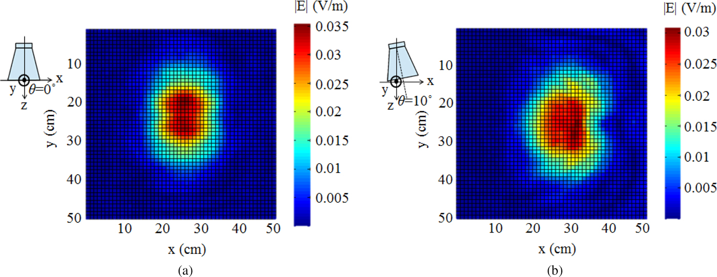
Fig. 6. Measured near-field data with 2601 data points for a 15-GHz horn antenna for θ values of (a) 0° and (b) 10°.
Figure 7 shows the simulated and measured absolute radiation patterns. The measured results for θ = 0° in both the E-plane (ϕ = 90°) and the H-plane (ϕ = 0°) are close to the corresponding simulated results. Thus, the baseline measurement results are validated. In Fig. 7(a), it is obvious that the main beam is shifted by 10° for an AUT angle of θ = 10°.

Fig. 7. Simulated and measured absolute radiation patterns of 15-GHz horn antenna in (a) H-plane and (b) E-plane.
The proposed method is subsequently applied to measure the near-field data. Figure 8 illustrates the near-field and the far-field data errors for the AUT at different θ values (0° and 10°) under constant ϕ (ϕ = 0°) with respect to the corresponding values of the measured points, respectively. The near-field and far-field data errors are calculated using (5),
 $${\rm data}\;{\rm error} = \displaystyle{{\sqrt {\sum\nolimits_x {\sum\nolimits_y { \vert {D_n}(x,\;y) - {D_{n - 1}}(x,\;y){ \vert ^2}}}}} \over {\sum\nolimits_x {\sum\nolimits_y {{D_{n - 1}}(x,\;y)}}}}, $$
where D n−1(x, y) denotes the data obtained by using the sampling theorem and D n (x, y) denotes the interpolated data obtained by using our method. The near-field and far-field data errors are 0% when the number of measured points is 2601 because all the measured points in the scanning plane are covered when following the sampling theorem. If a larger data error is acceptable, then the number of measuring points can be correspondingly reduced. In the case with θ = 0°, when measuring 781 points, the near-field data error is ~1.7% and the far-field data error is ~1.1%. The sampling points are subsequently reduced from 2601 to 781. In the case with θ = 10°, when measuring 912 points, the near-field data error is about 1.6% and the far-field data error is about 1.1%. The sampling points then reduce from 2601 to 912. In these two cases, the required measurements can be reduced by over 64.9%.

Fig. 8. (a) Near-field and (b) far-field data errors as functions of number of measured points.
Figure 9 shows the measured near-field data obtained with and without using the proposed method. It is observed that upon using the proposed method, the measured near-field pattern (using less data points) is nearly identical to that obtained with the sampling theorem for both cases.

Fig. 9. Measured near-field data alone with number of sampling points used as obtained by using (a) the sampling theorem and (b) the proposed method.
To discuss the difference on far-field pattern using different number of data points, the normalized radiation patterns are compared. The reference for the normalization is the maximum measured far-field pattern of θ = 0° using 2601 data points. All the pattern using the same reference for the normalization, therefore, the normalized radiation patterns are sufficient to verify the effect with different number of data points. Figure 10 shows the measured normalized radiation patterns for θ = 0° and 10°. The results obtained using three different numbers of data points are included to examine the effect of reducing the number of data points on the resulting antenna pattern. It is observed that the radiation patterns for the three cases are similar; this is because the far-field error is <1.1%, as shown in Fig. 8(b).

Fig. 10. Measured normalized radiation patterns of antenna for θ value of (a) 0° and (b) 10°.
Figure 11 shows the data point distribution for θ values of 0° and 10°. In comparison with the near-field distribution in Fig. 9, we observe that the measured points are dense (a large number of measurements) in the regions where the E-field varies rapidly (region A). In contrast, the measured points are sparse (fewer points) in the regions where the E-field changes smoothly (region B). Because a large portion of the measurement plane only requires sparse sampling, the number of measurement points significantly reduces.
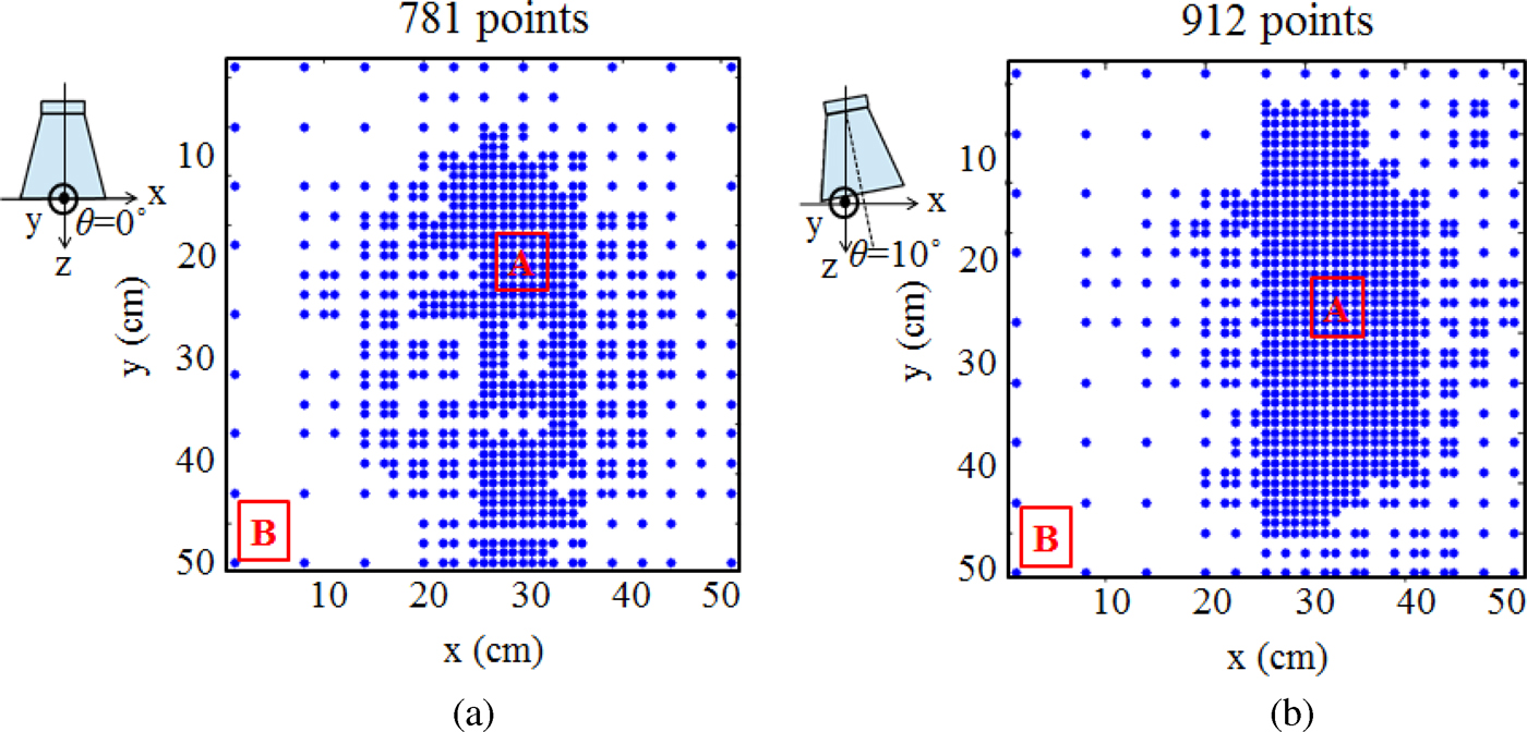
Fig. 11. Data point distribution obtained using the proposed method for θ value of (a) 0° and (b) 10°.
Table 1 summarizes the measured results. Upon comparing the numbers of data points required between the proposed method and sampling theorem, we note that the data point reduction is >64.9% with the proposed method. The reduction in the number of data points still only corresponds to near-field data variation (θ = 0° and θ = 10°) of <5%, which indicates that the performance of the proposed method does not change for two different patterns. This validates the robustness of our method.
Table 1. Performance summary of measured results.

V. CONCLUSION
In this study, we proposed a technique to reduce the time taken for near-field antenna measurements by reducing the number of measured points. The robustness of our method was validated with our measurement of a 15-GHz horn antenna oriented at different θ values (0° and 10°) under constant ϕ (ϕ = 0°). In the two corresponding measurement cases, the numbers of measured points were demonstrated to reduce from 2601 to 781 and from 2601 to 912. The reduction in the number of data points was >64.9%. Moreover, the data error between the measurement results obtained with the sampling theorem and the proposed method was below 1.7%. Thus, our proposed method can significantly reduce the number of data points to be measured while retaining the accuracy of the measured near-field data.
ACKNOWLEDGEMENT
This work is supported by Ministry of Science and Technology (contact no. NSC102-2221-E-194-017-MY3 and MOSP103-2622-E-194-008-CC1)
 Po-Jui Chiu is pursuing his M.S. in the Institute of Electrical Engineering at the National Chung Cheng University in Taiwan.
 Wei-Chung Cheng is pursuing his Ph.D. in the Institute of Electrical Engineering at the National Chung Cheng University in Taiwan.
 Zuo-Min Tsai was born in Maioli, Taiwan, in 1979. He received a B.S. degree 2001 from the Department of Electrical Engineering, National Taiwan University and a Ph.D. in communications engineering from the National Taiwan University, Taipei, Taiwan, in 2006. In July 2011, he joined the faculty of the Department of Electrical Engineering, National Chung Cheng University, where he is currently an Assistant Professor. His research interests include the design of microwave integrated circuits and microwave systems.
 Dong-Chen Tsai received an M.S. degree in Electrical Engineering from the National Chung Cheng University, Taiwan, in 2007. He is currently working toward the Ph.D. in the Graduate Institute of Communication Engineering, National Taiwan University. His research interests include image/video processing and video coding.


