I. INTRODUCTION
Microstrip structures of various shapes have recently received much attention due to the rapid growth in exploiting the millimeter-wave frequencies. They are very important in many commercial applications, such as mobile radio and wireless communications systems [Reference Barkat and Benghalia1, Reference Vasconcelos, Silva, Albuquerque, Oliveira and d'Assunção2].
During recent years, great interests have been shown in using a microstrip antenna deposited on the anisotropic substrate since the substrate anisotropy could have important applications for the operation of microstrip antennas [Reference Gurel and Yazgan3–Reference Fortaki, Khedrouche, Bouttout and Benghalia6]. With the increasing complexity of geometry and material property, designing these antennas requires more and more dedicated and sophisticated computer aided-design (CAD) tools to predict the characteristics. The method of moments (MoM) has been proven to be one of the most powerful CAD tools for solving this class of problems. By now, a number of microstrip antennas with the anisotropic substrate have been investigated using the MoM-based spectral domain analysis method [Reference Gurel and Yazgan3–Reference Boufrioua5].
In later studies on microstrip structures, anisotropic materials, especially the uniaxially anisotropic ones have been considered due to their advantages [Reference Djouablia, Messaouden and Benghalia7–Reference Messai, Benkouda, Amir, Bedra and Fortaki12]. It is known that some metamaterials exhibit uniaxial-type anisotropy both in permittivity and permeability tensors [Reference Benkouda and Fortaki13]. In the following designs of the rectangular and circular microstrips, metamaterials and other uniaxially anisotropic substrates have been used to obtain special operational characteristics.
In this paper, the effects of both electric and magnetic uniaxial anisotropy, in the substrate on resonant characteristics of the rectangular microstrip patch antenna are investigated. This subject has not been reported in the open literature: only the influence of the electric uniaxial anisotropy on the complex resonant frequency and bandwidth has been treated [Reference Zebiri, Lashab and Benabdelaziz4, Reference Fortaki, Djouane, Chebara and Benghalia14, Reference Fortaki and Benghalia15]. The present paper is organized as follows. In Section II, the derivations of the electric uniaxial Green's function in the spectral form, the associated moment method analysis of the complex resonant frequency of the printed antenna are presented. The calculation is performed by vector Fourier transforms, which gives rise to a diagonal form of the Green's function. The effects of the antenna parameters on resonant characteristics of the rectangular microstrip antenna are investigated in Section III. Variations in the permittivity perpendicular to the optical axis of the dielectric and along this axis are considered. Concluding remarks are summarized in Section IV.
II. SPECTRAL DOMAIN FORMULATION
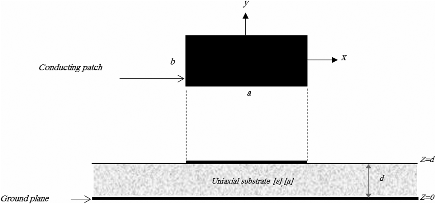
The rectangular microstrip patch antenna is shown in Fig. 1, along with the coordinate system used in the analysis. The microstrip patch is printed on a grounded uniaxial anisotropic dielectric slab with the optical axis normal to the patch. The permittivity and permeability tensors in this anisotropic region are given by
 $$\bar{\bf \varepsilon}=\varepsilon _0 \left[{\matrix{ {\varepsilon _x } & 0 & 0 \cr 0 & {\varepsilon _x } & 0 \cr 0 & 0 & {\varepsilon _z } \cr } } \right]\comma$$
 $$\bar{\bf \mu}=\mu _0 \left[{\matrix{ {\mu _x } & 0 & 0 \cr 0 & {\mu _x } & 0 \cr 0 & 0 & {\mu _z } \cr } } \right]\comma$$
where ε0 and μ0 are, respectively, the free-space permittivity and the free-space permeability. Equations (1) and (2) can be specialized to the isotropic substrate by allowing εx = εz = εr and μx = μz = μr. All fields and currents are time harmonic with the e iωt time dependence suppressed. The analysis needs three steps to obtain the resonant frequency and bandwidth of the rectangular microstrip antenna.

Fig. 1. Geometrical structure of a rectangular microstrip antenna.
A) Derivation of the dyadic Green's function
The transverse fields inside the anisotropic region (0 < z < d) can be obtained via the inverse vector Fourier transforms as shown in [Reference Fortaki, Djouane, Chebara and Benghalia14]
 $$\eqalign{{\bf E}\lpar {\bf r}_s\comma \; z\rpar & =\left[{\matrix{ {E_x \lpar {\bf r}_s\comma \; z\rpar } \cr {E_y \lpar {\bf r}_s\comma \; z\rpar } \cr } } \right]\cr & = \displaystyle{1 \over {4\pi ^2 }}\vint_{ - \infty }^{+\, \, \infty } {\vint_{ - \infty }^{+ \infty } {\bar{\bf F}\lpar {\bf k}_s\comma \; {\bf r}_s \rpar } } {\bf e}\lpar {\bf k}_s\comma \; z\rpar \, \, dk_x \, dk_y\comma \; }$$
 $$\eqalign{{\bf H}\lpar {\bf r}_s\comma \; z\rpar & =\left[{\matrix{ {H_y \lpar {\bf r}_s\comma \; z\rpar } \cr { - H_x \lpar {\bf r}_s\comma \; z\rpar } \cr } } \right]\cr & = \displaystyle{1 \over {4\pi ^2 }}\vint_{ - \infty }^{+\, \, \infty } {\vint_{ - \infty }^{+ \infty } {\bar{\bf F}\lpar {\bf k}_s\comma \; {\bf r}_s \rpar } } {\bf h}\lpar {\bf k}_s\comma \; z\rpar \, \, dk_x \, dk_y\comma \; }$$
where
 $$\eqalign{& \bar{\bf F}\lpar {\bf k}_s\comma \; {\bf r}_s \rpar = \displaystyle{1 \over {k_s }} \left[{\matrix{ {k_x } & {k_y } \cr {k_y } & { - k_x } \cr } } \right]e^{i\, {\bf k}_s .\, \, {\bf r}_s }\comma \; \quad {\bf r}_s=\hat{\bf x}\, x+\hat{\bf y}\, y\comma \; \cr & {\bf k}_s=\hat{\bf x}\, \, k_x+\hat{\bf y}\, k_y \comma \; \quad k_s=\left\vert {\, {\bf k}_s } \right\vert \comma}$$
 $${\bf e}\lpar {\bf k}_s\comma \; z\rpar =e^{ - \, \, i\, \, \bar{\bf k}_{z\, } \, z} \cdot {\bf A}\lpar {\bf k}_s \rpar +e^{i \bar{\bf k}_{z\, } z} \cdot {\bf B}\lpar {\bf k}_s \rpar \comma$$
 $${\bf h}\lpar {\bf k}_s\comma \; z\rpar =\bar{\bf g}\lpar {\bf k}_s \rpar \left[{e^{ - \, \, i\, \, \bar{\bf k}_{z\, } \, z} {\bf A}\lpar {\bf k}_s \rpar - e^{i\, \bar{\bf k}_{z\, } z} {\bf B}\lpar {\bf k}_s \rpar } \right].$$
In equations (6) and (7), A and B are two-component unknown vectors and
 $$\bar{\bf k}_z=\left[{\matrix{ {k_{z\, }^e } & 0 \cr 0 & {k_{z\, }^h } \cr } } \right]\comma \; \bar{\bf g}\lpar {\bf k}_s \rpar =\left[{\matrix{ {\displaystyle{{\omega \varepsilon _0 \varepsilon _x } \over {k_z^e }}} & 0 \cr 0 & {\displaystyle{{k_z^h } \over {\omega \mu _0 \mu _x }}} \cr } } \right]\comma$$
kze and kzh are, respectively, propagation constants for TM and TE waves in the uniaxially anisotropic substrate characterized by both permittivity and permeability tensors. They are given by
 $$\eqalign{& k_z^e=\sqrt {\displaystyle{{\varepsilon _x } \over {\varepsilon _z }}} \left({ \mu _x \varepsilon _z k_0^2 - k_s^2 } \right)^{{\textstyle{1 \over 2}}}\comma \; \quad k_z^h=\sqrt {\displaystyle{{\mu _x } \over {\mu _z }}} \left({ \mu _z \varepsilon _x k_0^2 - k_s^2 } \right)^{{\textstyle{1 \over 2}}}\comma \; \cr & k_0^2=\omega ^2 \varepsilon _0 \mu _0 .}$$
Writing equations (6) and (7) in the planes z = 0 and d, and by eliminating the unknowns A and B, we obtain the matrix form
 $$\left[{\matrix{ {{\bf e}\lpar {\bf k}_s\comma \; d^ - \rpar } \cr {{\bf h}\lpar {\bf k}_s\comma \; d^ - \rpar } \cr } } \right]=\bar{\bf T} \cdot \left[{\matrix{ {{\bf e}\lpar {\bf k}_s\comma \; 0^+\rpar } \cr {{\bf h}\lpar {\bf k}_s\comma \; 0^+\rpar } \cr } } \right]$$
with
 $$\bar{\bf T}=\left[{\matrix{ {\bar{\bf T}^{11} } & {\bar{\bf T}^{12} } \cr {\bar{\bf T}^{21} } & {\bar{\bf T}^{22} } \cr } } \right]=\left[{\matrix{ {\cos\lpar \bar{\bf k}_z d\rpar } & { - {\rm i }\bar{\bf g}^{ - 1} \cdot \sin \lpar \bar{\bf k}_z d\rpar } \cr { - {\rm i }\bar{\bf g} \cdot \sin \lpar \bar{\bf k}_z d\rpar } & {\cos \lpar \bar{\bf k}_z d\rpar } \cr } } \right]\comma$$
which combines e and h on both sides of the anisotropic region as input and output quantities. Now that we have the matrix representation of the anisotropic substrate characterized by both permittivity and permeability tensors, it is easy to derive the dyadic Green's function of the problem. The continuity equations for the tangential field components at the interface z = d are
 $${\bf e}\lpar {\bf k}_s\comma \; d^ - \rpar ={\bf e}\lpar {\bf k}_s\comma \; d^+\rpar ={\bf e}\lpar {\bf k}_s\comma \; d\rpar \comma$$
 $${\bf h}\lpar {\bf k}_s\comma \; d^ - \rpar - {\bf h}\lpar {\bf k}_s\comma \; d^+\rpar ={\bf j}\lpar {\bf k}_s \rpar \comma$$
j(ks) in equation (13) is related to the vector Fourier transform of J(rs), the current on the microstrip patch, as
 $${\bf j}\lpar {\bf k}_s \rpar =\vint_{ - \infty }^{+\infty } {\vint_{ - \infty }^{+\infty } {\bar{\bf F}\lpar {\bf k}_s\comma \; - {\bf r}_s \rpar } } {\bf J}\lpar {\bf r}_s \rpar dk_x \, dk_y\comma \; {\bf J}\lpar {\bf r}_s \rpar =\left[{\matrix{ {J_x \lpar {\bf r}_s \rpar } \cr {J_y \lpar {\bf r}_s \rpar } \cr } } \right].$$
The transverse electric field must necessarily be zero on a perfect conductor, so that for the ground plane we have
 $${\bf e}\lpar {\bf k}_s\comma \; 0^ - \rpar ={\bf e}\lpar {\bf k}_s\comma \; 0^+\rpar ={\bf e}\lpar {\bf k}_s\comma \; 0\rpar ={\bf 0}.$$
In the unbounded air region above the microstrip patch (d < z < +∞), the electromagnetic field given by equations (6) and (7) should vanish at z → +∞ according to the Sommerfeld's condition of radiation, yielding
 $${\bf h}\lpar {\bf k}_s\comma \; d^+\rpar =\bar{\bf g}_0 \lpar {\bf k}_s \rpar \cdot {\bf e}\lpar {\bf k}_s\comma \; d^+\rpar \comma$$
where  $\bar{\bf g}_0 \lpar \, {\bf k}_s \rpar $ can be easily obtained from the expression of
  $\bar{\bf g}\lpar {\bf k}_s \rpar $ given in equation (8) by allowing εx = εz = εr = 1 and μx = μz = μr = 1. Combining equations (10), (12), (13), (15), and (16), we obtain a j(ks) and e(ks, d) given by
 $${\bf e}\lpar {\bf k}_s\comma \; d\rpar =\bar{\bf G}\lpar {\bf k}_s \rpar \cdot {\bf j}\lpar {\bf k}_s \rpar \comma$$
where  $\bar{\bf G}\lpar {\bf k}_s \rpar $ is the dyadic Green's function in the vector Fourier transform domain, which is given by
 $$\bar{\bf G}\lpar {\bf k}_s \rpar =\left[{\matrix{ {G11} & 0 \cr 0 & {G22} \cr } } \right]=\left[{\bar{\bf T}^{22} .\left({\bar{\bf T}^{12} } \right)^{ - 1} - \bar{\bf g}_{\bf 0} } \right]^{ - 1} .$$
B) Integral equation formulation
The tangential electric field due to the surface current j can be expressed as
 $$E\lpar r_s\comma \; d\rpar =\displaystyle{1 \over {4\pi ^2 }}\vint_{ - \infty }^{+\infty } {\vint_{ - \infty }^{+\infty } {\bar F\lpar k_s\comma \; r_s \rpar \, \bar G\lpar k_s \rpar \, j\lpar k_s \rpar } \, dk_x \, dk_y } .$$
Enforcement of the boundary condition requiring the transverse electric field of (19) to vanish on the area of the microstrip patch yields the sought integral equation
 $$\vint_{ - \infty }^{+\infty } {\vint_{ - \infty }^{+\infty } {=\bar F\lpar k_s\comma \; r_s \rpar .\bar G\lpar k_s \rpar .j\lpar k_s \rpar \, dk_x \, dk_y \, 0\comma \; \lpar x\comma \; y\rpar \in {\rm patch}} } .$$
C) Galerkin's method solution of the integral equation
The first step in the Galerkin's method solution of equation (20) is to expand the patch current J(rs) into a finite series of the known basis functions J xn and J ym
 $${\bf J}\lpar {\bf r}_s \rpar =\sum\limits_{n=1}^N {a_n \left[{\matrix{ {J_{xn} \lpar {\bf r}_s \rpar } \cr 0 \cr } } \right]}+\sum\limits_{m=1}^M {b_m \left[{\matrix{ 0 \cr {J_{y m} \lpar {\bf r}_s \rpar } \cr } } \right]}\comma$$
where a n and b m are the mode expansion coefficients to be sought. Substitute the vector Fourier transform of equation (20) into (21). Next, the resulting equation is tested by the same set of basis functions that was used in the expansion of the patch current. Thus, the integral equation (20) is reduced to a system of linear equations, which can be written compactly in matrix form as [Reference Fortaki and Benghalia15, Reference Bouttout, Benabdelaziz, Fortaki and Khedrouche16]
 $$\left[{\matrix{ {\left({\bar{\bf Z}^{11} } \right)_{N \times N} } & {\left({\bar{\bf Z}^{12} } \right)_{N \times M} } \cr {\left({\bar{\bf Z}^{21} } \right)_{M \times N} } & {\left({\bar{\bf Z}^{22} } \right)_{M \times M} } \cr } } \right]\cdot \left[{\matrix{ {\left({\bf a} \right)_{N \times 1} } \cr {\left({\bf b} \right)_{M \times 1} } \cr } } \right]={\bf 0}\comma$$
where the elements of the impedance matrix  $\left({\, \bar{\bf Z}} \right)_{\, \lpar N\, \hskip --1pt +\, \, M\rpar \, \, \times \, \, \lpar N\, \, +\, \, M\rpar } $ are given by
 $$\left({\bar{\bf Z}^{11} } \right)_{kn} =\vint_{ - \infty }^{+\infty } {\vint_{ - \infty }^{+\infty } {\displaystyle{ 1 \over {k_s^2 }}\lsqb k_x^2 G11+k_y^2 G22\rsqb \tilde J_{xk} \lpar \!\!- {\bf k}_s \rpar \tilde J_{xn} \lpar {\bf k}_s \rpar \, dk_x \, dk_y\comma \; } }$$
 $$\eqalign{\left({\bar{\bf Z}^{12} } \right)_{km}=& \vint_{ - \infty }^{+\infty } {\vint_{ - \infty }^{+\infty } {\displaystyle{{k_x k_y } \over {k_s^2 }}\lsqb G11\! - \!G22\rsqb } } \tilde J_{xk} \cr & \lpar \!\!- {\bf k}_s \rpar \tilde J_{ym} \lpar {\bf k}_s \rpar dk_x dk_y\comma}$$
 $$\eqalign{\left({\bar{\bf Z}^{21} } \right)_{ln}= & \vint_{ - \infty }^{+\infty } {\vint_{ - \infty }^{+\infty } {\displaystyle{{k_x k_y } \over {k_s^2 }}\lsqb G11 - G22\rsqb } } \tilde J_{yl} \cr & \lpar \!\!- {\bf k}_s \rpar \tilde J_{xn} \lpar {\bf k}_s \rpar \, dk_x \, dk_y\comma}$$
 $$\eqalign{\left({\bar{\bf Z}^{22} } \right)_{lm}=& \vint_{ - \infty }^{+\infty } {\vint_{ - \infty }^{+\infty } {\displaystyle{ 1 \over {k_s^2 }}\lsqb k_y^2 G11+k_x^2 G22\rsqb } } \tilde J_{yl} \cr & \lpar \!\!- {\bf k}_s \rpar \tilde J_{ym} \lpar {\bf k}_s \rpar \, dk_x \, dk_y .}$$
 In equations (23)–(26),  $\tilde J_{x n} $ and
  $\tilde J_{y m} $ are the scalar Fourier transforms of J xn and J ym, respectively. For the existence of a non-trivial solution of equation (22), we must have
 $$\det \left[{\bar{\bf Z}\left(\omega \right)} \right]=0.$$
Equation (27) is an eigenequation for ω, from which the characteristics of the structure of Fig. 1 can be obtained. Let ω = 2π(f r + if i) be the complex root of equation (27). In that case, the quantity f r stands for the resonant frequency, the quantity BW = 2f i/f r stands for the half-power bandwidth and the quantity Q = f r/(2f i) stands for the quality factor.
III. NUMERICAL RESULTS AND DISCUSSION
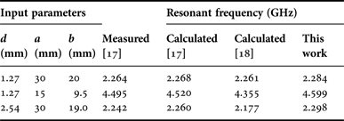
To check the accuracy of the spectral domain method described in the previous section for electric anisotropic case, our results are compared with an experimental and theoretical values presented in the previous work [Reference Pozar17, Reference Aouabdia, Belhadj-Tahar, Alquie and Benabdelaziz18]. The convergent resonant frequencies for different substrate thicknesses are in an excellent agreement with the experiment results (Table 1).
Table 1. Comparison of calculated and measured resonant frequencies, for a rectangular microstrip patch in a uniaxial electric anisotropic substrate (εx = 13.0, εz = 10.2).
The resonant frequency and bandwidth of the patch antenna against substrate thicknesses for different electric anisotropy ratio (AR 1 = εx/εz) are shown in Figs 2(a) and 2(b). It is observed that the resonant frequency shift to higher values in the case of positive anisotropic (AR 1 < 1) and smaller in the case of the negative anisotropy (AR 1 > 1). Therefore, the effect of electric anisotropy is more pronounced for the thick substrate than for the thin substrate. This is attributed to the fact that for the thick substrates, in addition to TM propagating waves, TE waves will also be excited, which results in an increasing of dependency of the resonant frequency on εx and consequently on AR 1. Thus, it can be concluded that the effect of uniaxial electric anisotropy on the resonant frequency of a rectangular microstrip patch antenna cannot be ignored and must be taken into account in the design stage.
Fig. 2. Variation of the resonant frequency and half-power bandwidth of the rectangular patch versus substrate thicknesses for different values of the anisotropy ratio, εz = 2.43, a = 19 mm, b = 22.9 mm, and μx = μz = 1, when εx is changed.
From Fig. 2(b), it can also be observed that to increase the half-power bandwidth, the electric anisotropy ratio must be adjusted to a value less than unity. As an example, the decrease of AR 1 from 1 to 0.5 results in an increase in the bandwidth of about 1.55%. With the aim of providing further increase in the half-power bandwidth, the substrate thickness can be increased. This method cannot, however, be extended too far without the loss of the highly desirable low-profile characteristics of the rectangular antenna. Another problem that arises when the substrate becomes electrically thick is the surface wave excitation, which affects the antenna performance.
Now, the effects of uniaxial magnetic anisotropy on the resonant frequency and the bandwidth characteristics are determined as a function of the magnetic anisotropy ratio (AR 2 = μx/μz). It is obvious that the magnetic anisotropy ratio takes the value 1 for the isotropic case. In Fig. 3(a), resonant frequency shift due to increase in substrate thicknesses for different magnetic anisotropy ratios is shown. The value of the relative permeability perpendicular to the optical axis is fixed at μx = 2.4. To adjust the magnetic anisotropy ratio, the relative permeability along the optical axis (μz) is varied. The dielectric permittivity of the substrate is taken as (εx = 3.25, εz = 7.25). The parameters of the rectangular patch are chosen to be identical to those considered in Figs 2(a) and 2(b). It is observed in the figure that in the cases of (AR 2 < 1), incremental shift is observed in the resonant frequency, whereas in the case of (AR 2 > 1) detrimental shift is observed. Therefore, the effect of magnetic anisotropy is significant only for the thick substrates.
Fig. 3. Variation of the resonant frequency and half-power bandwidth of the rectangular patch versus substrate thicknesses for different values of the anisotropy ratio, μx = 2.4, a = 19 mm, and b = 22.9 mm, (εx = 3.25, εz = 7.25), when μz is changed.
In Fig. 3(b), the bandwidth of the patch antenna against the substrate thicknesses for different magnetic anisotropy ratio is shown. It is observed from this figure that to enhance the bandwidth of the rectangular antenna, magnetic anisotropy ratio must be adjusted to a value larger than unity (AR 2 = 1). To provide an additional increase in the half-power bandwidth, the substrate thickness can be increased. Note that, although the enhancement of the bandwidth can be achieved by means of the adjustment of AR 1 or AR 2, the adjustment of AR 2 is the best way since it allows a very significant improvement in the bandwidth of the rectangular microstrip patch antenna.
The resonant frequency and bandwidth shifts of the antenna with increasing patch length are shown in Figs 4(a) and 4(b). In these figures, relative permittivity values along the non-optical axes are taken equally as (εx = 2.43) and the substrate thickness as (d = 1.59 mm). In this case, optical axis permittivity is used for the adjustment of the anisotropy ratio. It is observed in Fig. 3(a) that when the anisotropy ratio is adjusted to 0.5 (AR 1 = 0.5), the resonant frequency takes a smaller value with respect to the isotropic case (AR 1 = 1) and slightly decreases with increasing patch length. The opposite situation is observed when the anisotropy ratio has increased to 2 (AR 1 = 2) by decreasing the optical axis permittivity. In this case, the resonant frequency value and its shift with respect to the isotropic case increase in increasing the patch length. These results indicate that the effect of increasing patch length on the resonant frequency becomes more significant with respect to the isotropic case for higher anisotropy ratio values.
Fig. 4. Resonant frequency and bandwidth versus patch length for different electric anisotropy ratio values (AR 1 = εx/εz), a = 19 mm, εx = 2.43, d = 1.59 mm, μx = μz = 1, when εz changed.
The situation is similar for the bandwidth as observed in Fig. 4(b). The results in this figure indicate that the bandwidth of the rectangular patch microstrip antenna can be increased several times with respect to the isotropic case depending on the adjustment of the anisotropy ratio and patch length.
The resonant frequency and bandwidth shifts of the antenna with an increasing patch length for different values of the magnetic anisotropy ratio (AR 2) are shown in Figs 5(a) and 5(b). In Fig. 5(a), the resonant frequency versus the length of rectangular patch is shown. In this figure, the relative permittivity value is taken as (εx = εz = 2.43), relative permeability values along the optical axes are taken equally as (μz = 2.4), and substrate thickness as (d = 1.59 mm). It is observed in the figure that if the magnetic anisotropy ratio is adjusted to a smaller value than one (AR 2 < 1), the resonant frequency increases. The opposite is true when the anisotropy ratio is greater than the unity. These results indicate the main effect of the substrate anisotropy and patch length on the resonant frequency of the rectangular microstrip patch.
Fig. 5. Resonant frequency and bandwidth versus patch length for different magnetic anisotropy ratio values (AR 2 = μx/μz), a = 19 mm, μz = 2.4, d = 1.59 mm, εx = εz = 2.43, when μx changed.
The results in Fig. 5(b) indicate that the bandwidth of the rectangular patch microstrip antenna can be increased several times with respect to the isotropic case depending on the adjustment of the anisotropy ratio and patch length.
IV. CONCLUSION
We have described an accurate analysis of rectangular microstrip antenna with anisotropic substrates. The uniaxially anisotropic medium shows anisotropy of an electric type as well as anisotropy of a magnetic type. The extended spectral-domain integral equation with the Galerkin moment method solution combined with the concept of the complex resistive boundary condition have been used to solve for the resonant frequency, half-power bandwidth of the antenna structure. Both permittivity and permeability tensors of the anisotropic substrate have been included in the formulation of the dyadic Green's function of the problem. The accuracy of the method was checked by performing a set of results in terms of resonant frequencies for various anisotropic substrate materials. In all cases, very good agreements compared with the literature were obtained. The results indicate that the effect of increasing patch length on the resonant frequency becomes more significant with respect to the isotropic case for higher anisotropy ratio values. Computations show that uniaxial electric anisotropy as well as uniaxial magnetic anisotropy affects the resonant characteristics of the rectangular antenna and consequently they must be taken into account in the design stage. The effect of electric and magnetic anisotropy is more pronounced for the thick substrate than for the thin substrates. So the results indicate that the bandwidth of the rectangular patch microstrip antenna can be increased several times with respect to the isotropic case depending on the adjustment of the anisotropy ratio and patch length. This behavior agrees with that of discovered experimentally for rectangular patches on the isotropic or electric anisotropic substrates [Reference Aouabdia, Belhadj-Tahar, Alquie and Benabdelaziz18]. According to the results, it seems to be possible to maintain control of the resonant frequency and obtain wide-band operation using uniaxial substrate having properly selected both permittivity and permeability along the optical and the non-optical axes combined with optimally chosen structural parameters.
APPENDIX
Although the full-wave analysis can give results for several resonant modes [Reference Fortaki, Djouane, Chebara and Benghalia14, Reference Bouttout, Benabdelaziz, Fortaki and Khedrouche16], only the results for the TM01 mode are presented in this study. The basis functions for the following numerical calculations are selected to be sinusoidal functions of
 $$J_{xk} \lpar x\comma \; y\rpar =\sin \left[{\displaystyle{{k_1 \pi } \over a}\left({x+\displaystyle{a \over 2}} \right)} \right]\cos \left[{\displaystyle{{k_2 \pi } \over b}\left({y+\displaystyle{b \over 2}} \right)} \right]\comma$$
 $$J_{ym} \lpar x\comma \; y\rpar =\sin \left[{\displaystyle{{m_2 \pi } \over b}\left({y+\displaystyle{b \over 2}} \right)} \right]\cos \left[{\displaystyle{{m_1 \pi } \over a}\left({x+\displaystyle{a \over 2}} \right)} \right].$$
Note that the modes are now identified by the integer doublet k 1k 2 (m 1m 2) instead of k(m). This type of basis function is very appropriate for the vector Fourier transform domain analysis of rectangular microstrip patches for three reasons: (1) they ensure a quick convergence of the Galerkin's method in the vector Fourier transform domain with respect to the number of basis functions; (2) they lead to vector Fourier transform domain infinite integrals, which are amenable to asymptotic analytical integration techniques; and (3) their vector Fourier transforms can be obtained in the closed form [Reference Fortaki, Djouane, Chebara and Benghalia14–Reference Bouttout, Benabdelaziz, Fortaki and Khedrouche16].
The Fourier transforms of J xn and J ym are
 $$\tilde J_{xk}=\vint_{ - \infty }^{+\infty } {\vint_{ - \infty }^{+\infty } {J_{xk} \exp \lpar - ik_x x - ik_y y\rpar \, dx\, dy} }\comma$$
 $$\tilde J_{ym}=\vint_{ - \infty }^{+\infty } {\vint_{ - \infty }^{+\infty } {J_{ym} exp\lpar - ik_x x - ik_y y\rpar \, dx\, dy} } .$$
From equations (A1) and (A2), the basic functions from the model of the cavity are
 $$J_{xk} \lpar x\comma \; y\rpar =\sin \left[{\displaystyle{{k_1 \pi } \over a}\left({x+\displaystyle{a \over 2}} \right)} \right]\cos \left[{\displaystyle{{k_2 \pi } \over b}\left({y+\displaystyle{b \over 2}} \right)} \right]\comma$$
 $$J_{ym} \lpar x\comma \; y\rpar =\sin \left[{\displaystyle{{m_2 \pi } \over b}\left({y+\displaystyle{b \over 2}} \right)} \right]\cos \left[{\displaystyle{{m_1 \pi } \over a}\left({x+\displaystyle{a \over 2}} \right)} \right].$$
Substituting (A5) into (A3) and (A6) into (A4) and after some mathematical operations, we obtain the following expressions for scalar transforms Fourier J xk and J ym:
 $$\tilde J_{xk}=\tilde I_{xx} \lpar k_x \rpar \cdot \tilde I_{x y} \lpar k_y \rpar \comma$$
 $$\tilde J_{ym}=\tilde I_{yx} \lpar k_x \rpar \cdot \tilde I_{y y} \lpar k_y \rpar$$
with
 $$\eqalign{{{\tilde I}_{xx}} & = \displaystyle{{ia} \over 2}\lsqb \exp \lpar - i{k_1}\pi /2\rpar \cdot \sin {\rm c}\lpar {k_x}a/2 + {k_1}\pi /2\rpar \cr & - \exp \lpar i{k_1}\pi /2\rpar \cdot \sin {\rm c}\lpar {k_x}a/2 - {k_1}\pi /2\rpar \rsqb \comma \; }$$
 $$\eqalign{{{\tilde I}_{xy}}& = \displaystyle{b \over 2}\lsqb \exp \lpar - i{k_2}\pi /2\rpar \cdot \sin {\rm c}\lpar {k_y}b/2 + {k_2}\pi /2\rpar \cr & + \exp \lpar i{k_2}\pi /2\rpar \cdot \sin {\rm c}\lpar {k_y}b/2 - {k_2}\pi /2\rpar \rsqb \comma}$$
 $$\eqalign{ {{\tilde I}_{yx}} & = \displaystyle{a \over 2}\lsqb \exp \lpar - i{m_1}\pi /2\rpar \cdot \sin {\rm c}\lpar {k_x}a/2 + {m_1}\pi /2\rpar \cr & + \exp \lpar i{m_1}\pi /2\rpar \cdot \sin {\rm c}\lpar {k_x}a/2 - {m_1}\pi /2\rpar \rsqb \comma \; }$$
 $$\eqalign{{{\tilde I}_{yy}} & = \displaystyle{{ib} \over 2}\lsqb \exp \lpar - i{m_2}\pi /2\rpar \cdot \sin {\rm c}\lpar {k_y}b/2 + {m_2}\pi /2\rpar \cr & - \exp \lpar i{m_2}\pi /2\rpar \cdot \sin {\rm c}\lpar {k_y}b/2 - {m_2}\pi /2\rpar \rsqb .}$$
Mourad Hassad received Engineer and Master Science degrees both in Electronics from the University of Batna, Algeria, in 2006 and 2009, respectively. He is currently working toward the Ph.D. degree at the University of Batna, Algeria. His current research activities include on microstrip structures, anisotropic materials, and especially the magnetic–electric uniaxially anisotropic media.
Sami Bedra was born on 3 August 1984 in Batna, Algeria. He obtained the Engineer and Master Science degrees both in Electronics from the University of Batna, Algeria, in 2008 and 2011, respectively. He is currently working toward the Ph.D. degree at the University of Batna, Algeria. His current research activities include neural network, optimization techniques, and their applications to patch antennas.
Randa Bedra was born on 9 September 1989 in Batna, Algeria. She received the Master Science degree in Microwave and Telecommunications from the University of Batna, Algeria, in 2013. She is currently with the Laboratory of Advanced Electronics at Electronics Department, University of Batna, Batna, Algeria. She is currently working toward the Ph.D. degree at the University of Batna. Her main research deals with numerical methods and microstrip antennas.
Siham Benkouda was born on 30 August 1983 in Arris, Algeria. She received the Master Science and Ph.D. degrees in Electronics Engineering from the University of Batna, Algeria, in 2008 and 2012, respectively. She is currently with the Laboratory of ultrahigh frequencies and semiconductors at Electronics Department, University of Constantine 1, Constantine, Algeria. Her main research deals with numerical methods and microstrip antennas.
Akrame Soufiane Boughrara was born on 30 June 1974 in Constantine, Algeria. He received the Engineer of Communication degree from the University of Constantine, Algeria, in 1999, the Master Science degree in Microwaves from the University of Batna, Algeria, in 2011. He is currently working toward the Ph.D. degree at the University of Batna, Algeria. His current research activities include modeling and design of microstrip structure resonator.
Tarek Fortaki was born on 31 March 1972 in Constantine, Algeria. He received the Engineer of Communication degree in 1995, the Master Science degree in Microwaves in 1999, and the Doctorate degree in Microwaves in 2004, all from Electronics Department, Faculty of Engineering Science, University of Constantine, Constantine, Algeria. Currently, he is a Professor at the Electronics Department, Faculty of Engineering Science, University of Batna, Algeria. He has published 17 papers in refereed journals and more than 40 papers in conference proceedings. He serves as a reviewer for several technical journals. His main interests are electromagnetic theory, numerical methods, and modeling of antennas and passive microwave circuits.