I. INTRODUCTION
Many applications depend on 24/7 monitoring devices to image wide areas in harsh environmental conditions. For instance, daylight mining requires a permanent observation of hillsides to predict landslides. Also in case of disasters, such as an earthquake, or a structural collapse, a monitoring system can be used to support rescue teams in finding injured or passed out humans. Such a system can not only be used in finding people but also in protecting the rescuers by observing the damaged structures to predict for instance a collapse of partial structures. In this case, it is important to recognize changes in the observed scene over a distinct time period to detect and analyze small movements to predict upcoming risks like further collapses of damaged buildings. LASER devices could in principle be used to measure movements in the range of millimeters, however, they fail if the atmosphere is obscured for instance by rain, fog, smoke, dust, or sand storms. Additionally, sand, blown by the wind, can blind their sensitive optics within minutes. Radar systems are able to penetrate an intransparent atmosphere, making them ideal measurement tools in rough weather conditions. Especially in complex scenarios, an imaging radar system has many benefits. The spot of interest does not have to be known in prior to the operator (e.g. an instable roof of a damaged building) because an imaging radar system illuminates the whole area. Furthermore, the remote sensing capability of radar makes it an ideal choice for areas where a direct access is not possible. The MIMO technique offers some benefits compared to a fully filled phased-array radar system. The number of receive and transmit elements can be reduced by √N, with N the number of elements in a phased array radar. This helps to reduce the costs and the weight. Also the physical dimension in azimuth can be reduced by a factor of 2 with respect to a phased array without decreasing the spatial resolution. This makes the radar system more compact for mobile usage. In addition to existing imaging MIMO radar systems which are specialized for short-range applications [Reference Gumbmann, Tran, Weinzierl and Schmidt1] or which work as a frequency modulated continuous wave (FMCW) radar [Reference Zwanetski and Rohling2], MIRA-CLE Ka is able to be used for short- and mid-range applications and can easily be configured for several radar modes.
II. SYSTEM SPECIFICATIONS
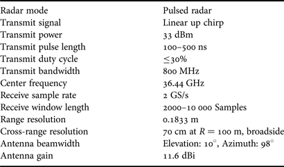
The system parameters used for the measurements presented in this paper are shown in Table 1. These are typical parameters which are capable for most scenarios mentioned above. Since the system is highly configurable, several parameters, e.g. the transmit pulse length or the receive window length are only limited by the used hardware. The system offers the possibility of a quick selection of several parameters, e.g. bandwidth, center frequency, or pulse length to adapt the system in real time to changing observation conditions.
Table 1. MIRA-CLE Ka parameters.

The range resolution is given by
 $$\delta R = \displaystyle{{c_0 } \over {2B}}$$
and the azimuth resolution for broadside can be approximated by
 $$\delta y \approx R\displaystyle{{\rm \lambda } \over {l_{bistatic} }}\comma$$
with l bistatic as the length of the virtual bistatic array, which is nearly twice the size of the real antenna array, c 0 the speed of light, B the bandwidth, λ the wavelength, and R the distance in range.
III. HARDWARE SETUP
The radar system is separated into a high-frequency frontend and a backend in order to be highly portable with a high degree of flexibility. The complete system is shown in Fig. 1. The cables, connecting the frontend with the backend, were removed for the picture. A block diagram of the radar frontend with its main components is shown in Fig. 2. The frontend is mounted on a very stable tripod to operate the system safely, with reliable radar measurements also on uneven surfaces, and without vibrations (e.g. caused by wind), or other external influences.
Fig. 1. The MIMO radar MIRA-CLE Ka.
Fig. 2. Block diagram of the MIRA-CLE Ka frontend.
A) Signal upconversion
The inserted IF signal is upconverted by a single sideband mixer with a LO frequency of 4 GHz. The required 90° hybrid on the IF path for sideband selection is realized externally to ensure the flexibility of the module. The mixer suppresses the lower side band by 30 dB. After this, the signal is filtered and then multiplied two times by a factor of two with one following filter for each doubler stage. The output frequency can be calculated by
 $$f_{up} = 4\lpar f_{in} + f_{LO_{up} } \rpar \comma$$
with f up the output frequency of the upconverter, f in the IF input from the arbitrary waveform generator in the backend, and f LO up the local oscillator frequency for the upconverter. For the presented results the IF signal is a linear chirp from 505 to 605 MHz so that the output generates a linear chirp from 18.02 to 18.42 GHz. These values ensure that the carrier and lower sideband are located far enough from the desired frequency band to be attenuated by the integrated filters. Currently the bandwidth of this module is limited to 600 MHz of output bandwidth. There is a new upconverter module developed which will be implemented soon and offers an output bandwidth of 1 GHz to achieve a transmit bandwidth of 2 GHz. A picture of the currently used module is shown in Fig. 3. The LO signal is connected to the left, the IF signal and the 90° phase-shifted IF signal are inserted on the upper part and the output is on the right side. The PCB is separated into two parts: the high frequency part on the upper part and the power and digital part on the lower side [Reference Wilden, Klare, Fröhlich and Krist3–Reference El-Arnauti, Saalmann and Klare5].
Fig. 3. Signal upconverter of MIRA-CLE Ka without 90° hybrid on the IF side.
B) Transmitter
The first stage of the transmitter is a low-noise amplifier that amplifies the input signal to compress the following frequency doubler. After multiplication the signal is filtered by a third-order interdigital filter with a center frequency of 36 GHz and a bandwidth of 10 GHz. These filters ensure that the undesired harmonics of the input frequency are strongly attenuated. The transmit frequency is calculated by
 $$\eqalign{& f_{TX} = 2f_{up}\comma \; \cr & f_{TX} = 8\lpar f_{in} + f_{LO_{up} } \rpar \comma}$$
with f TX the output frequency of the transmitter. To compensate the losses of the filter and of the transmission line, another gain driver is implemented. A high-power amplifier, to achieve the desired output power, is the last stage before the antenna. Also the high-power amplifier operates in compression to achieve the most possible output power. All active RF parts can be switched on and off externally via an LVDS connection. The transmitted radar pulse of 33 dBm is radiated by an antenna with a gain of 11.6 dBi. The transmitter was developed with the requirement to fit in a spacing of nearly half the wavelength of the center frequency. With a maximum duty cycle of 30% the transmitter is very flexible for future radar modes which uses, for instance waveform diversity. For the presented results the inserted signal is a linear chirp from 18.02 to 18.42 GHz. The signal linearly sweeps from 36.04 to 36.84 GHz after the doubler stage. A full view of an assembled transmitter block is shown in Fig. 4. On the backside there is only one coaxial connector for the IF signal and on the top side there are the connectors for the digital signals and the power supply [Reference Nzouatom6].
Fig. 4. Ka band transmitter block of MIRA-CLE Ka.
C) Receiver
The homodyne receiver uses a sub harmonically pumped mixer for downconversion. From this follows that the LO has to be half the RF and only one LO is needed. The output of the receiver is calculated by
 $$f_{IF} = f_{RX} - 2f_{LO_{RX} }\comma$$
with f IF the output frequency of the receiver, f RX the RF input frequency, and f LO RX the local oscillator frequency for the receiver. For the presented results, the LO frequency was fixed to 18 GHz and the received linear chirp was mixed down to an intermediate frequency of 40–840 MHz. Due to the design of the frontend the LO input of the receiver can alternatively be connected with the output of the upconverter to realize an FMCW operation. This allows a lower sampling rate of the digitizers and a higher energy of the transmitted signal due to its longer pulse. The first stage after the antenna is an LNA with a noise figure of 2.5 dB to keep the system noise as low as possible. After the LNA the signal is filtered, attenuated by an RF attenuator, and then mixed down. The IF path consists of two wideband amplifiers and a variable attenuator. The radio frequency (RF) attenuator and the intermediate frequency (IF) attenuator are controlled by a microcontroller which is externally connected via USB port to the workstation. With both attenuators the system gain can be programmed between 14 and 54 dB. Each receiver has its own ID and can be controlled individually. All active parts in the receiver are switchable externally via an low voltage differential signaling (LVDS) connection as the transmitter. The complete receiving module has a single sideband noise figure of about 3 dB without the antenna. Currently, the receiver is used as an IF downconverter but it is prepared to be used also as an in-phase quadratur (IQ) downconverter. In combination with two digitizing channels for each receiver the bandwidth can be increased without increasing the sampling rate of the analog to digital converter. A full view on an equipped receiver PCB without the antenna is shown in Fig. 5. The antenna is directly connected on the left part of the PCB. The LO signal is connected to the central coaxial connector on the right side of the receiver and the inphase and quadrature phase outputs are on the upper and lower coaxial connectors. On the upper side of the PCB the digital signals are connected and on the lower right side the power is applied [Reference Wilden, Klare, Fröhlich and Krist3, Reference Fröhlich7].
Fig. 5. Receiver of MIRA-CLE Ka.
D) Current monitoring
All temperature sensitive modules are monitored by an additional current monitoring system to protect them against overheating in case of failure. These monitors are designed so that the duty cycle or the maximum pulse length of the transmitters does not reach a critical level. The state of each module and its temperature is displayed on an LC panel, mounted on the backside of the frontend. In addition to the temperatures this module also monitors the voltages in the frontend to prevent failures or damages caused by undervoltages or overvoltages.
E) Radiator
The receive and transmit antennas, which are used in MIRA-CLE Ka, are identical for the transmitters and the receivers. As it was important to fill a virtual array with a spacing of nearly half the wavelength, the packaging density of the used antennas had to be very high. Each single antenna is designed as an array of 8 Vivaldi elements in elevation and ensures a very slim size in azimuth. Only the thickness of the substrate limits the dimensions of the antenna. The used Vivaldi antenna array is polarized vertically. With this design the achieved 3 dB beamwidth of a single RX/TX antenna reaches 10° in elevation and 98° in azimuth direction. For different beamwidthes in elevation the antenna can easily be reconfigured by adding or deleting Vivaldi elements per array. Only the distribution network to the antenna elements has to be adopted to match the impedance of the TX and RX modules which is about 50 Ω. The gain of one column with 8 elements is 11.6 dBi. The input matching of the antennas between 30 and 40 GHz is below −10 dB. The design of the antenna can be seen on a fully equipped block with 8 transmitters in Fig. 4 [Reference Wilden, Klare, Fröhlich and Krist3].
F) Antenna array design
MIRA-CLE Ka uses the same number of TX and RX elements in order to reduce the number of elements to the minimum. With N TX = 16 and N RX = 16 a total number of virtual elements N virtual = N TXN RX = 256 is generated. In MIRA-CLE Ka two blocks of transmit arrays are used, one on each side of the receive array. With this constellation, the size of the virtual array is nearly twice the size of the physical array. For the transmit array, the achieved spacing between the elements is 0.58λ. To get an equidistant spacing between the virtual elements (d virt = d TX) the distance for the receiving elements results to d RX = 8d TX and the receive and transmit arrays are placed in a distance of d TX/RX = d TX/2. The total length of the virtual array results in l bistatic = 255d virt. A full view of the array is shown in Fig. 6. Due to this design the length of the virtual bistatic array l bistatic = 1248 mm determines the azimuth resolution of about 0.4° which results in a cross range resolution of about 70 cm in the 100 m range in broadside [Reference Klare, Saalmann, Wilden and Brenner8]. All transmit and receive elements are screwed on a rail and can be moved to any possible position on this rail in order to analyze different array constellations. So, the system has the possibility to realize special thinned array designs in the future [Reference Rezer9].
Fig. 6. MIMO array inside the frontend.
G) Oscillators
In the frontend two oscillators are present. One oscillates at 4 GHz and is required by the upconverter in the transmit path and for the clock of the arbitrary waveform generator in the backend which operates at 4 GS/s. The other one oscillates at 18 GHz and is needed to supply the subharmonic mixer in the receivers. The frequency output of the oscillator operating at 4 GHz is generated directly by a dielectric resonator oscillator. The other oscillator is build up by the 4 GHz clock in addition with a quartz oscillator operating at 500 MHz and using them in combination with another upconverter module. In addition with an external 90° hybrid and selecting the upper sideband the desired 18 GHz is achieved. For this oscillator the same upconverter as for transmission is used (f up = 4 · (f in + f LO up)). All oscillators are locked to the 10 MHz master clock located in the backend to guarantee the coherence.
H) Miscellaneous
In addition to the described modules there are some more parts in the frontend which are necessary for operation. The distribution of the signal from the upconverter to the transmitter and the distribution of the 18 GHz local oscillator to the receivers, both need a distribution network from 1 input to 16 outputs and both are at about 18 GHz. Due to the spatial arrangement of the MIMO array each distribution is equipped with a 1 to 2 power divider and two 1 to 8 dividers to achieve the required number of outputs. Because of the unidirectionality of the distributed signals the power dividers were designed as Wilkinson dividers. To compensate the losses of the cables and to keep the noise at a low level additional amplifiers are integrated in the signal paths. In the receive path four 4 to 1 switches are integrated in the signal path to multiplex the 16 channels of the receive modules to the 4 channels of the analog to digital converters.
The main parts, which have been integrated in the backend, are shown in Fig. 7.
Fig. 7. Block diagram of the MIRA-CLE Ka backend.
I) Backend rack
To ensure the systems mobility, all components of the backend were placed into a 19 inch rack. This configuration allows a transportation in a small van or a large passenger car. A monitor and a keyboard are integrated in the rack to fully control the radar system and to display the radar image. The power supply is completely integrated in the backend rack. Due to the field of applications the system can be supplied by a diesel powered electric generator. It was important to chose power supplies which are very resistant to rippled input power or voltage surges.
J) Workstation
The backend is equipped with a high performance workstation. This computer controls the waveform generator, the AD converter, the pattern generator, and the attenuator settings of the receivers. The main program on the workstation is written in MATLAB. It initializes and controls the distributed hardware. To get a quick view of the illuminated scene, an online processor has been integrated. At this moment two different modes of processing are implemented. One is for imaging and it can be selected if the image is plotted in polar or in cartesian coordinates. For the online processing mode a broadband beamforming process is implemented. This is necessary to avoid the squinting of a narrowband beamforming processing over the bandwidth. The broadband beamforming process is realized in the frequency domain and for every look angle each frequency is shifted by a calculated phase. This process is the digital equivalent to a beamsteering with true time delays in a phased array instead of using phase shifters. Another mode is the change detection mode in which very low changes in the illuminated scene can be displayed. Currently it is possible to process about one image per second, depending on the scene. The acquired data are stored on a hard disk for later processing. It is implemented that the user can select between an online processing, data acquisition, or both. The high resolution signal processing is done offline in order to get the best possible image quality [Reference Klare and Saalmann10].
K) Pattern generator
The pattern generator operates as the central sequence controller, which initiates the beginning of a MIMO cycle and controls the power supply of the transmit and receive elements in the frontend. It also triggers the waveform generator and sets the states of the switches in the frontend, which forward the signals from the receivers to the AD converter. LVDS signals are used to ensure a stable and undisturbed communication of the pattern generator and the high-frequency frontend. The pattern consists of one MIMO cycle and is triggered by the workstation. The pattern itself is calculated by the workstation on the basis of the dimensions of the illuminated scene. To ensure the system coherence the clock of the pattern generator is locked by the 10 MHz master clock.
L) Signal generation
The generation of the IF transmit signal is performed by an arbitrary waveform generator. The arbitrary waveform generator from the manufacturer chase scientific instruments is implemented as an expansion card in the workstation. With this configuration it is easy to expand the current setup by additional arbitrary waveform generators. To have a high flexibility for different experimental conditions, it is equipped with a 4 GS/s DA-converter and 16 MS of memory. For MIRA-CLE Ka the digital to analog converter is clocked by a synchronous external 4 GHz clock to generate a coherently clocked waveform. The external clock is needed because the internal 4 GHz oscillator cannot be locked to an external 10 MHz reference signal. Due to the available memory the longest possible waveform is limited to 4 ms. In addition to the analog output, the arbitrary waveform generator (AWG) card is equipped with two transistor-transistor-logik (TTL) marker outputs. One of these markers is used to trigger the digitizer to reach the best possible coherence of the data acquisition to the transmitted signal. As described in A and B, the bandwidth of the generated signal is multiplied by a factor of 8 before transmission. Currently the analog output generates a linear chirp with a bandwidth of 100 MHz to achieve 800 MHz of transmit bandwidth.
M) Data acquisition
The AD converters, which are also implemented in the backend, can simultaneously record four channels with a data rate of 2 GS/s. The digitizers from Agilent offer the possibility to choose between different acquisition modes. Besides the option of sampling four simultaneous channels at 2 GS/s, the AD digitizer has the ability of sampling two channels at 4 GS/s or one channel at 8 GS/s. When using four channels, only 64 acquisitions are needed to fully fill the complete virtual array. In the following, each fully filled virtual array is called a MIMO cycle. During a MIMO cycle the recorded data are cached in the random-access memory (RAM) of the analog digital (AD) converter. The acquisition of one MIMO cycle lasts 1.28 ms. With a range resolution of 0.1833 m and a cross-range resolution of 70 cm at 100 m range the sampling rate in the fast time domain and the sampling rate of one MIMO cycle results that an object has to move with a radial speed of 143 m/s to change from one resolution cell to the other or with a speed of 547 m/s in crossrange to change the azimuthal resolution cell. This makes this system even with time multiplexing feasible for a wide range of applications. Also there is the possibility of using special switching schemes for a MIMO radar using time multiplexing to reduce the effects of defocussing in azimuth of moving objects if one has to deal with faster objects [Reference Guetlein, Bertl, Kirschner and Detlefsen11]. To keep the azimuthal grating lobes of the beamformed image at an acceptable level, the maximum phase change during one MIMO cycle has to be below 20°. Because of the periodicity in the MIMO array, 20° of phase change would result in a grating lobe level of about −30 dB. This results in a radial velocity of 0.536 m/s for the illuminated object.
After each MIMO cycle, the recorded data are sent to the workstation via high-speed data link. This means that the length of the recording is only limited by the size of the hard drive in the workstation. In case of a standard scenario with 10 000 recorded samples per pulse and per virtual element and a resolution of 10 bit per sample, each MIMO cycle generates raw data of about 3 MB. To improve the signal-to-noise ratio (SNR), several MIMO cycles can be recorded for a coherent averaging. This operation is done by the workstation. In addition to the variable attenuators, integrated in the receivers, the full scale level of the digitizer can be adjusted between 50 mV and 5 V, so the variable gain of the receive path rises by 40 to 80 dB.
N) Master clock generation
The master clock is realized with an oven-controlled quartz oscillator with 10 MHz and is implemented in the backend. To ensure the coherence of the whole system, all time critical components in the backend and in the frontend are referenced to this clock. For change measurements in the observed scene the stability of this clock is sufficient for detecting changes of about 0.1 mm over a few hours.
IV. CALIBRATION
For the calibration of the system, a far-field method was used. To get the transfer function of each virtual element, the reflections of all 256 TX/RX combinations of a corner reflector have been recorded. This corner reflector was placed in a low reflecting environment exactly orthogonal to the MIMO array. To receive strong echoes, the radar was placed 30 m away from the reflector. Because of the short distance between radar and reflector the pulse width was reduced to 100 ns. The setup for this calibration is shown in Fig. 8.
Fig. 8. Calibration setup of MIRA-CLE Ka without the radome.
To achieve the 256 complex transfer functions, the following steps were performed: at first the received raw data of the corner reflector were Fourier transformed and divided by the reference transmit signal. Then the obtained signals were transformed to the time domain and were cut with a rectangular window that only the echoes of the corner reflector were integrated in the transfer functions. The achieved transfer functions were then padded with zeros to the length of the recorded scene and Fourier transformed. The raw data of the recorded scene are inverse filtered with these transfer functions. Due to the height of the corner reflector a completely static target cannot be assured because of oscillations of the tripod resulting from windy conditions during the calibration measurements. To eliminate the movement of the corner reflector over the time enough recordings had to be integrated to receive a good transfer function.
V. RESULTS
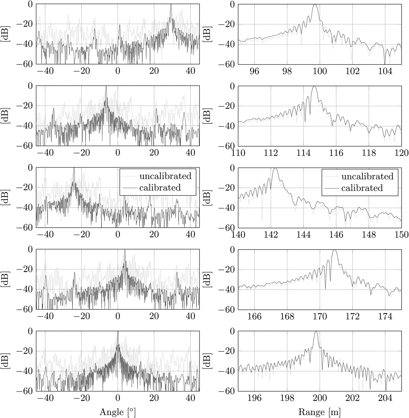
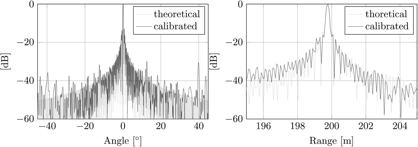
To verify that the received transfer functions were valid, a field of five corner reflectors was set up. The reflectors were placed in several range and azimuth lines. A cut in azimuth of the corner reflectors of the beamformed image is shown in Fig. 9. For better comparison of the data, the calibrated and uncalibrated data have been normalized. The side lobes and the grating lobes are strongly decreased by the calibration process. The highest grating lobe can be found at −30 dBc, for the corner reflector in broadside at 200 m range, and the first side lobes are nearly exact at −13 dBc. The 3 dB beamwidth of 0.34° is also at the theoretical beamwidth of 0.34°. A comparison of the calibrated result and the theoretical one is shown in Fig. 10. For this comparison the corner reflector in broadside at 200 m range is analyzed. The difference between the calibrated result and the theoretical one in azimuth is caused by the mutual coupling of the edge elements of the transmitters. The differences in range, especially in the direction toward the radar, results because of the tripod, where the corner reflector is mounted on, which is not perfectly absorbing the incident electromagnetic wave. Also the fact that the corner reflector is not a perfect point scatterer influences the results. A cut in range of the corner reflectors is shown in Fig. 9. The first side lobes are also nearly −13 dBc and the further side lobes decreases inversely proportional to the distance of the reflector. The 3 dB resolution in range of 0.172 m is only 6% larger than the theoretical one of 0.1613 m. The final processed image of the scene is shown in Fig. 11. The range compression was performed by a wideband beamforming process. Both were processed in frequency domain. This figure shows the data in Cartesian coordinates which had to be transformed from polar coordinates. All processing is done without any tapering window. If a wider mainlobe can be accepted an appropriate window function can be applied to reduce the sidelobes. The calculated positions of the corner reflectors were compared with the measured positions of the corner reflectors by GPS. By integrating several thousand measurements with every GPS unit, measurement errors of about 0.5 m could be achieved. Due to the tolerance of the global positioning system (GPS) additional measurements with a LASER were performed. To obtain positions in azimuth and range also from far distance corner reflectors, triangulation was used for the one-dimensional LASER measurements. The error of one LASER measurement is 1 mm. These results verified the calculations on the processed data.
Fig. 9. Cut in azimuth (left) and range (right) of the beamformed image (Fig. 11), showing the corner reflectors in ascending range.
Fig. 10. Cut in azimuth (left) and range (right) of the beamformed image (Fig. 11), showing the corner reflector at 200 m range.
Fig. 11. Field of five corner reflectors in dB.
VI. CONCLUSION AND OUTLOOK
With MIRA-CLE Ka a MIMO radar in Ka band was successfully built up, which is ready to use in a few minutes, and can be transported by a small van or even in a larger passenger car. The robust design of the system, and the stationary imaging capability without any movements, predestines MIRA-CLE Ka for being used under rough conditions. The calibration process shows that the system is able to perform an image of the observed scene with a grating lobe level of −30 dBc in azimuth and a nearly perfect matching in range. The long-term coherence of the system makes MIRA-CLE Ka a good tool for analyzing very slow movements or changes in the illuminated scene. The results of a change detection measurement have already been published [Reference Klare, Saalmann and Biallawons12].
One of the next steps in the near future will be to perform experiments in more realistic scenarios.
For the future it is planned to increase the sampling rate of the AD converters. In the first step, the sampling rate will be increased to 4 GS/s to achieve a usable bandwidth of 2 GHz that delivers a range resolution of 7.5 cm. Later the sampling rate will be increased to 8 GS/s which will result in a range resolution of 3.75 cm. For the upgrades a new signal upconverter will be integrated in the system [Reference El-Arnauti, Saalmann and Klare5] because of the bandwidth limitation of the currently integrated upconverter. By increasing the bandwidth the number of analog-to-digital converters will be increased, too. To extend the configurability, additional switching matrices will be implemented in the intermediate frequency path of the receivers. With this upgrades there will be an option to switch between a high-resolution mode and a mode with a reduced number of transmit cycles to fill the virtual array by digitizing more parallel receive channels at once.
It is also planned to add more arbitrary waveform generators. They will be programmed with orthogonal waveforms in time- and frequency domain to reduce the number of pulses required to fully fill the virtual array. For this kind of diversity different waveforms will be verified in several conditions to fit the requirements. It will also be possible to use frequency multiplexing. This will also be used to reduce the number of required acquisitions to fill the virtual array. In case of using the radar in an FMCW mode it is possible to use frequency multiplexing without decreasing the bandwidth for each channel. This can be realized by using a frequency offset for each transmitter which is greater than the maximum beat frequency of the observed scene. In this configuration, the receivers can separate each transmitter [Reference Pfeffer, Feger, Schmid, Wagner and Stelzer13, Reference de Wit, van Rossum and de Jong14].
It is also possible to use the linear array on a moving platform, e.g. like an airplane, and use the synthetic aperture radar (SAR) principle to generate a three-dimensional image. In this application, the MIMO array has to be orthogonal to the movement vector of the platform and also orthogonal to range. So, the resolution in azimuth is generated by the synthetic aperture and the resolution in elevation in generated by the MIMO array. The resolution in range is still generated by the time of arrival of the electromagnetic waves [Reference Klare, Brenner and Ender15–Reference Gumbmann and Schmidt17]. To realize a three-dimensional image without any movable parts it is possible to upgrade the linear MIMO array to a planar array [Reference Koeppel, Methfessel, Schiessl and Schmidt18, Reference Zhuge and Yarovoy19].
 Oliver Biallawons received his diploma in Electrical Engineering from the University of Siegen, Siegen, Germany in 2011. He now is working for the Fraunhofer Institute for High Frequency Physics and Radar Techniques in the Department of Array-based Radar Imaging and the team “MIMO-Radar and Multistatics”. His main research interests are system design and signal processing for MIMO radar Systems.
 Jens Klare received the diploma in Physics from the Ruprecht-Karls-Universität Heidelberg, Heidelberg, Germany, in 1998 and carried out his diploma thesis at the Max-Planck-Institute for Astronomy in Heidelberg. He received his Ph.D. degree in astronomy from the Rheinische Friedrich-Wilhelms-Universität Bonn, Bonn, Germany, in 2003. He performed his Ph.D. thesis at the Max-Planck-Institute for Radio Astronomy in Bonn, with the investigation of active galactic nuclei, supermassive binary black hole systems, and ultra-relativistic plasma jets using very long baseline interferometry (VLBI) at highest frequencies and space-VLBI at longest baselines. From 2003 to 2004 he was a postdoctoral research fellow at the Max-Planck-Institute for Radio Astronomy in Bonn, Germany.
In 2004, he joined the Fraunhofer Institute for High Frequency Physics and Radar Techniques FHR, Wachtberg, Germany. Since 2009 he is the team leader of the team “MIMO-Radar and Multistatics”. His current research interests include MIMO radar, MIMO SAR, bi- and multi-static SAR, 3D radar imaging, and waveform diversity. Dr. Jens Klare is a member of IEEE, Information Technology Society ITG of the Association for Electrical, Electronic & Information Technologies VDE, European Microwave Association EuMA, and German Physical Society DPG.
 Olaf Saalmann received his diploma in Electrical Engineering from the University of Applied Sciences, Koblenz, Germany, in 1989. He joined the Department of Array-based Radar Imaging, Institute for High Frequency Physics and Radar Techniques (FHR) where he is currently active in high resolution imaging radar technology. His areas of interest are the design of new broadband scanning radar systems and MIMO radar.