II. SPECTROGRAM GENERATION

A spectrogram is a two-dimensional (2D)-graphical “waterfall” representation of the spectral content of a signal as function of time, where the power level in each time–frequency cell is taken from a color or gray scale. The appearance of a spectrogram depends on waveform and processing parameters, which will be discussed next.

A spectrogram is obtained by taking the magnitude squared of the short-time Fourier transform (STFT) of a discrete signal, where the STFT can be written as:

(1) $${\rm STFT}\left\{ {x\left[ n \right]} \right\} \equiv X(m,k) = \mathop \sum \limits_{n = - \infty} ^\infty x\left[ n \right]w\left[ {n - m} \right]e^{ - (j2\pi kn/N)}.$$

Here, x[n] is the discrete signal, w[n] is the discrete window function, which is non-zero in [0..N] and zero elsewhere, n is the sample number, N is the number of samples in the analysis window, and k is an index for the frequency kω ₀, where ω ₀ = 2πf _s /N with sample rate f _s . For radars measuring range and Doppler, f _s in this paper is sometimes referred to as pulse repetition frequency (PRF) in case of pulse radars and sweep repetition frequency (SRF) in case of frequency-modulated continuous-wave (FMCW) radars. Index m determines the position of the analysis window. By repeatedly calculating the STFT with increasing m using a certain step size Δm, the spectrogram can be obtained. The step size Δm can be chosen such that a certain overlap between two consecutive analysis windows is realized, which gives a smoother result in the time dimension. Each calculation of the STFT gives a single column in the spectrogram, which will be referred to as a “trace”.

If we want to generate a visually useful spectrogram of a certain event, such as the flapping of a bird's wing, then we need to choose an appropriate value for N. As a rule of thumb, we should choose to have the integration interval N/f _s as a fraction of the length of the event. This we refer to as the “short integration interval”. The wing beat period of the majority of bird species in steady flight is in the range of 0.05–0.5 s [Reference Pennycuick2]. By assuming a moderate wing beat period of 0.1 s, the suitable integration interval to capture the details of a single wing beat cycle is of the order of 20 ms. The maximum radial velocity associated with flapping wings is about 15 m/s depending on the aspect angle. Consequently, the required sample rate f _s is relatively low, i.e. several kilohertz in X-band. A spectrogram of a flying bird, measured with an X-band continuous-wave (CW) radar, is shown in Fig. 1. For different bird species the spectrogram will appear different, e.g. in terms of wing beat frequency and amplitude, but comparable in terms of wing beat modulation around the (usually stronger) body echo.

Fig. 1. Measured spectrogram of a bateleur (Terathopius ecaudatus)

Compared with flapping wings, spinning rotor blades constitute much faster events with much higher associated velocities. The rotor rotation period of mini-UAVs is of the order of milliseconds with related blade tip velocities of perhaps 200 m/s or even higher. The required sample rate f _s is therefore very high, of the order of tens of kilohertz. With a CW radar, such high sample rates are achievable, as well as with some short-range surveillance radars. Considering typical medium and long-range surveillance radars, however, such a high sample rate is unfeasible.

For periodic events that are stable to some extent, such as the spinning of rotor blades, “long integration intervals” can be applied for generating the spectrogram. By applying longer integration time, several revolutions of the rotor blades are included. The instantaneous spectral content is now dominated by the rotation rate of the blades causing modulation peaks. The instantaneous radial velocity of the blade tips is no longer observable. The difference between short and long integration interval is clearly visible in the measured spectrograms shown in Fig. 3 (top left and right). In case of long integration time, under sampling (i.e. lower sample rates) can be allowed if “cepstral analysis” is applied, as will be discussed in the next section.

III. CEPSTROGRAM GENERATION

Cepstral analysis can be used to assess the rate of change in a spectrum and it has been used for, e.g. characterizing seismic echoes from earth quakes and for human speech analysis. Cepstral analysis is based on the power cepstrum, which is defined as the power of the inverse Fourier transform of the logarithm of the power spectrum [Reference Bogert, Healy, Tukey and Rosenblatt3]. Congruently to the STFT and spectrogram, a short-time cepstrum [Reference Noll and Schroeder4] and “cepstrogram” have been proposed:

(2) $${\rm CG}\left\{ {x\left[ n \right]} \right\}\left( {m,k} \right) = \left\vert {{\rm \cal F}^{ - 1} \left\{ {^{10} \log \left( {\left\vert {{\rm STFT}\left\{ {x\left[ n \right]} \right\}\left( {m,k} \right)} \right \vert^2} \right)} \right\}} \right \vert^2,$$

in which ℱ⁻¹ is the inverse Fourier transform. Also here, the calculation of CG for a single m is referred to as a “trace” and corresponds to a single integration interval of N samples. The running variable of the cepstrum has the dimension of seconds and has been coined “quefrency”. The micro-Doppler periodicity expressed in hertz can be obtained by taking the inverse of the quefrency.

The cepstrogram will prove particularly valuable in the case of long integration interval measurements on rotor or propeller-driven targets. We can use it to determine the micro-Doppler periodicity, which is related to the blade flash frequency, which in turn is related to the angular velocity of the rotor or propeller (see Fig. 3 and the Discussion). We can determine whether we deal with a single rotor or multicopter-type target (see Fig. 4 and the Discussion). In clear cases, we can even estimate the number of rotors and their individual angular velocities.

To further demonstrate the potential of the cepstrogram, we point out the natural cyclic property of the inverse Fourier transform in equation (2). This property allows for extracting the micro-Doppler periodicity even in case of under sampling. The micro-Doppler periodicity feature is sufficient to discriminate man-made objects and bio-life. Consider the following simulation of a mini-UAV with four rotors each with two blades of 12 cm length. The average rotation rate is 80 rounds per second (RPS), with 6 RPS difference between the rotors. In addition, 3 RPS variance has been added to each rotor to account for some minor steering dynamics over time. Now, let us assume an X-band radar with a sampling rate of only 3 kHz, corresponding to practical range-Doppler surveillance operation. The blind velocity in X-band is around ±22.5 m/s, whereas the blade tip velocity is 60.3 m/s, so significant aliasing occurs. This prohibits the extraction of the overall micro-Doppler spectrum width. However, if we monitor the cepstrogram, we can still identify the micro-Doppler periodicity, as is shown in Fig. 2. Since the extracted quefrencies are very low, between 4.5 and 7 ms, the target can be classified as man-made.

Fig. 2. Spectrogram (left) and cepstrogram (right) from a simulated stationary target with four rotors and two blades per rotor. Radar sample rate is 3 kHz.

IV. APPLICATION ON REAL MEASUREMENTS

A low-power experimental CW radar operating in X-band was used to acquire measurements on real life targets. In Fig. 3, a measurement on a small radio-controlled (RC) helicopter is shown. The micro-Doppler spectrum width is clearly visible in the long integration interval and appears quite constant. The short integration interval reveals a relative slowly rotating, even-bladed main rotor and a much faster rotating, yet shorter second rotor (the tail rotor), also even-bladed [Reference de Wit, Harmanny and Prémel-Cabic5]. Both rotors are also visible in the cepstrogram, with the main rotor producing the strongest signal at 20.6 ms quefrency, which corresponds to approximately 24 RPS for the two-bladed main rotor. This value is appropriate for this particular RC helicopter.

Fig. 3. Long and short integration interval spectrograms (top) of an RC helicopter shown bottom left. The cepstrogram is shown bottom right.

An octocopter example is shown in Fig. 4. The short integration interval in the top right panel now appears chaotic due to the superposition of eight asynchronous rotors. The long integration interval does reveal the micro-Doppler spectrum width and quite some dynamics in the separate harmonics, but the periodicity cannot be deduced from the spectrogram. The cepstrogram however shows clear quefrency peaks between 4.5 and 6.5 ms, corresponding to rotation rates of 76.9 RPS up to 111.1 RPS considering two-bladed rotors. This range of values is appropriate for this particular octocopter. From the cepstrogram it is clear that the rotation rates of the different rotors are continuously adapted to keep the octocopter stable in the wind.

Fig. 4. Long and short integration interval spectrograms (top) of an RC octocopter shown bottom left. The cepstrogram is shown bottom right.

V. RELEVANT FEATURES

Suitable features provide information on target parameters and are discriminative between relevant target classes. For reliable classification under varying conditions, features should be robust with respect to target type, radar settings, and measurement parameters, such as carrier frequency, sample rate, polarization, and aspect angle. In this section, the relevant micro-Doppler features for classification of birds and mini-UAVs are reviewed, i.e. RCS, overall target velocity, micro-Doppler periodicity and micro-Doppler spectrum width.

In general, the RCS of mini-UAVs is higher than that of birds (depending on the species). RCS is therefore a discriminative feature, but it is not a robust feature. Observed RCS levels fluctuate significantly as function of aspect angle and radar frequency. One reason is that small and medium-sized birds and mini-UAVs are in the Mie resonance region for S- and X-band radar frequencies.

Typically, the main velocity component in a spectrogram is due to the motion of a target as a whole, assuming the body or fuselage gives the strongest reflection. Velocity components due to moving parts are usually weaker. The velocity of birds and many types of mini-UAVs is in the same range, such that radial velocity is not that much discriminative. Also, radial velocity is not a robust feature in itself since it depends on direction of flight with respect to the radar.

Many target micro-motions are of periodic nature, i.e. the pendulum-like motion of a bird's wings and the rotation of rotor/propeller blades. The related spectrograms are periodic as well. The period of a mini-UAV spectrogram is determined by the rotor rotation rate, which is generally one order of magnitude higher than that of manned helicopters. The period of a bird spectrogram is related to the wing beat cycle. The wing beat frequency of birds is between 2 and 20 beats per second, depending on the species. The periodicity of mini-UAVs can be extracted using cepstral analysis, as was discussed in Section III. In case of multiple dominant components in the spectrogram, for instance with multicopters, we can take the average periodicity (within a single trace). Furthermore, if we consider the periodicity values from multiple traces, we can calculate the variance or standard deviation on the average periodicity (from trace to trace). For multicopters we expect to find higher variance as compared with helicopters. This is because of the multiple dominant components in the cepstrogram, but also because the rotation rates of the individual rotors are continuously and rapidly adapted in order to manoeuvre and stabilize the platform. For helicopters the blade flash frequency is much more stable. Note this difference in Figs 3 and 4.

The micro-Doppler spectrum width indicates the maximum velocity of the micro-motions relative to the main velocity component. This feature can be exploited to distinguish birds from mini-UAVs. The spectrum width associated with flying birds is just several meters per second. Typically, the velocity spread related to spinning rotors is much wider. The spectrum width feature is robust with respect to radar parameters, but it depends on the target aspect angle. High sample rates are necessary to obtain the unambiguous Doppler spectrum from mini-UAVs. Note that for range-Doppler radar, this means using specific classification waveforms with a very high PRF or SRF, as was discussed in Section II.

VI. FEATURE EXTRACTION AND CLASSIFICATION

In the remainder of this paper, we will work toward a classifier example that uses the features mentioned in Section V. All features except for spectrum width as we assume that we are unable to measure this feature with a radar that operates with a relatively low f _s in the spectral dimension, i.e. <10 kHz. This radar does however give us at least range and accompanying Doppler-spectrum for the unknown object. Our primary goal is to be able to make a quick distinction between a man-made object and (possible) bio-life, based on a single “scan” over the target, i.e. single time-on-target that consists of several traces. In the second step, in case of a man-made object, we would like to be able to indicate a certain subclass, e.g. whether it is a kind of helicopter or a multicopter, etc.

We try to obtain the following information for a certain number of traces M (e.g. M = 10), which will become our feature vector for classification:

1. (1) Mean radar cross section, $\overline {rcs} \; \left[m^2\right]$ .

2. (2) Target speed, V _body (m/s).

3. (3) Mean dominant periodicity, for each trace, μ _periodicity [Hz].

4. (4) Standard deviation on the mean periodicity from several traces, σ _periodicity [Hz].

The mean RCS for a detected target is obtained by: $\overline {rcs} = \displaystyle{1 \over M}\sum\nolimits_{i = 1}^M {C_i R_i^4 \displaystyle{{S_i} \over {N_i}}}$ .

S _i /N _i is the signal to (thermal) noise ratio of the main body, which is usually the strongest bin in the Doppler-spectrum outside the stationary clutter band. C _i is a radar and waveform-dependent constant, containing items such as transmit power, antenna gain, number of pulses, etc. In cases where these factors are constant for all M measurements, we may instead use C = C _i for i = 1,…, M. Similarly, for a radially slow or stationary target, the range is constant R = R _i .

If the main body can be identified in the Doppler spectrum, then the radial velocity of the target can be extracted. Combined with the heading of the target, we may find the absolute speed V _body . If the heading is not known, then we may use the absolute value of the radial velocity for V _body instead, but then one should allow all classification models to have zero velocity as the target may fly tangentially.

The mean periodicity is obtained from the cepstrum. Different approaches can be used, but in our case we will do the following.

1. (1) Calculate the cepstrum for each trace using equation (2). We will use only the first half, i.e. N/2 samples, as both halves share the same content. Let q _i be the quefrency for each cell, equal to q _i = (i − 1)/f _s in seconds. Let p _i be the cepstral value for cell i, with i = 1,…, N/2. In our case, we will identify the quefrencies by their index, and refrain from interpolation between cells. Note that typically p _i ≫ for low i as these cells cover a relative large bandwidth. For Gaussian input noise, the resulting noise distribution will appear ∝1/q _i . For this reason, we will not use the first n − 1 samples, i.e. Q _all = {n,…, N/2}.

2. (2) Apply a noise threshold, $Q_T = \left\{ {i \in Q_{all} \vert\; p_i \gt \left[c_1 /q_i \right] + c_2} \right\}$ , where c ₁ and c ₂ are tuning constants to set the threshold performance.

3. (3) From the threshold crossings, find the mean peaks, i.e. local maxima, $Q_{LM} = \left\{ i \in Q_T \; \vert \nexists j \in Q_T : p_i \lt p_j \wedge \left \vert {i - j} \right \vert = 1 \right\}.$

4. (4) Find the fundamental quefrencies, called “fundamentals”. Often, the cepstrum shows harmonics for each fundamental. These are called “rahmonics”. We need to assess all items in Q _LM and decide whether they are a fundamental or a rahmonic. The following algorithm can be used for each separate trace:

   1. (a) Parameters and initialization: Let F be a variable set of fundamentals, initialized to F := Ø. Let α be a decision parameter for assessing whether two quefrencies match, set to, e.g. α = 1. Let β be a decision parameter for assessing whether a fundamental has been found, set to, e.g. β = 0.5 Let Π be the maximum rahmonic we consider to be visible in the data, set to, e.g. Π = 4.

   2. (b) Main algorithm:

      1. (i) If Q _LM = Ø, then stop, else, take a quefrency index k∈Q _LM and set the current rahmonic under consideration r to r := Π.

      2. (ii) If r < 0, then go to step i.

         Else, assess whether k is the rth rahmonic, in which case the fundamental f∈Q _all would be at f = [k/(r + 1)]. Local maxima hits would be expected at H = {nf∈Q _all |n=1..(r + 1)|}. The following hits actually match the measurement $H^{\prime} = \left\{ {h \in H \vert\exists y \in Q_{LM} :\; \left \vert {h - y} \right \vert \le \alpha} \right\}.$

      3. (iii) If we found sufficient proof, i.e. #H′/(r + 1) > β, then we update F := F∪{f} and $Q_{LM} : = \{ y \in Q_{LM} \vert \nexists s \in \{ 1..(r + 1)\} :\; \left \vert {s - y} \right \vert \le \alpha \}$ , and go to step i, else, we assume r := r − 1, and go to step ii.

5. (5) The fundamentals for the current trace are indexed in F. These correspond to the periodicities 1/q _k [Hz] with k∈F. The result is subject to the overall resolution of the cepstrum 1/f _s .

6. (6) Finally we take,

   (3) $$\mu_{\rm periodicity} = \displaystyle{\sum\nolimits_{f \in F} \sum\nolimits_{k = 0}^{\rm \Pi} 1/q_{(k + 1)_f} \cdot p_{(k + 1)f} \over \# F \cdot \sum\nolimits_{f \in F} \sum\nolimits_{k = 0}^{\rm \Pi} p_{(k + 1)f}.} \;$$

The standard deviation of the periodicity σ _periodicity is simply obtained by σ _periodicity = std(μ _periodicityi ) with i = 1..M.

For each radar time-on-target (i.e. the time the radar beam touches the target), consisting of M traces, of (overlapping) integration intervals of N samples, we obtain a feature vector ${\bi z}$ , composed of, ${\bi z} = \left[ {rcs,\; V_{body}, \mu _{periodicity}, \; \sigma _{periodicity}} \right]^T$ , which is then fed to the classifier.

For the sake of demonstration, we will take one of the simplest forms of classifiers, which is the MAP probability classifier, also known as the “unit cost function Bayesian”, or “minimum error rate” classifier [Reference van der Heijden, Duin, de Ridder and Tax6]. Here, the decision function $\hat \omega _{MAP} ( \cdot ):\; {\rm \opf R}^N \to {\rm \Omega} $ , that maps the feature vector ${\bi z} \in {\rm \opf R}^N $ to a class ω _i ∈Ω, with i∈{1..K}, is obtained by $\hat \omega _{MAP} ({\bi z}) = \mathop {{\rm argmax}}\limits_{\omega \in {\rm \Omega}} \left\{ {p({\bi z}\vert\omega )P(\omega )} \right\}$ .

The conditional probability density functions $p({\bi z} \vert \omega _k )$ contain the discriminative information, while the priors P(ω) carry information on the composition of the entire population. Quite often however, the priors are chosen to be equal, i.e. P(ω) = 1/K. Of course, in practice we could use the priors to influence our classifier, e.g. in areas with migrating birds in order to reduce the false alarm rate.

The $p({\bi z}\vert\omega _k )$ functions can be found using training sets and a generative learning algorithm, but it is not uncommon to just simply define them ad hoc using some a priori knowledge from the targets. In our case, we intend to implement the following aspects:

1. (1) We are only interested in small targets that can contain either bio-life or man-made targets. Aerial target larger than, say, 0 dBm² are considered to be man-made, but need no further detailing.

2. (2) Among the small aerial targets, helicopters and multicopters are more-or-less in the same velocity bracket as birds, but fixed wing aircraft can go a lot faster.

3. (3) Given the chosen features, we should be able to tell apart drone helicopters, from drone fixed wing aircraft, from drone multicopters. For instance, for drone helicopters, we could argue that their blade flash frequency can be quite low compared with propeller carrying targets. And multicopters might have quite some variance on theirs, compared to helicopters and fixed wing aircraft.

4. (4) In absence of clear distinctive features obtained from the cepstrogram, we should conclude that no propellers or rotors are “seen” by the radar, thus the target could be anything ranging from a bird to any type of drone. Still, all bio-life will fall into this category.

Our set of classes Ω is thus chosen as follows:

Ω = {“largeManMade”, “possibleBioLife”, “smallFixedWing Type”, “smallHeliType”, “smallMulticopterType”}.

Instead of using a training set to shape up the target models in terms of features, we will stick to experience based, hand drawn linear likelihood curves in which we expect certain targets to appear. Because we are using features that have a physical meaning, we are able to mold the knowledge we have of our targets regarding these features, directly into the classifier. To illustrate this approach, the curves of the smallHeliType are shown in Fig. 5. From this we can, e.g. see the low σ _periodicity that we would expect from an RC helicopter, whereas for a multicopter, this value is expected to be much higher.

Fig. 5. Model of small model helicopters, with a single dominant rotor that gives a fairly low, yet stable blade flash frequency.

VII. CLASSIFICATION RESULTS

Several drone and bird measurements were given as input to the classifier from Section VI. Three results are shown in Figs 6 and 7 for an octocopter measurement, Figs 8 and 9 for an RC helicopter measurement and Figs 10 and 11 for a bird measurement.

Fig. 6. Left: spectrogram of an octocopter measurement. Right: cepstrogram of an octocopter measurement. “X” markers indicate the chosen fundamentals.

Fig. 7. Classification result of an octocopter measurement. Only classes that appear at least once are shown.

Fig. 8. Left: spectrogram of an RC helicopter measurement. Right: cepstrogram of an RC helicopter measurement.

Fig. 9. Classification result of an RC helicopter measurement. Only classes that appear at least once are shown.

Fig. 10. Left: spectrogram of a bird measurement. Right: cepstrogram of a bird measurement (no detections here)

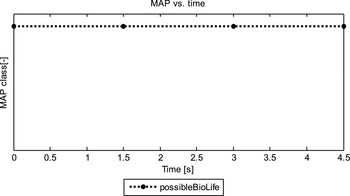
Fig. 11. Classification result of a bird measurement. Only classes that appear at least once are shown.

The white markers on the left panels of Figs 6, 8 and 10 indicate for each trace the bin with the strongest signal excluding the clutter band from −1 to +1 m/s. This corresponds, most of the time, with the radial body velocity of the target. If the target crosses the clutter band, then wrong values are chosen, which for this particular example is not critical. The spectrograms of Figs 6 and 8 also show the long integration interval micro-Doppler signal as lines following the body signal. For the bird in Fig. 10 spectrogram wingbeat modulation is visible around the main body.

The right panels of Figs 6, 8 and 10 show the corresponding cepstrograms. In these figures, the chosen fundamentals according the algorithm in Section VI are indicated by white markers. For Fig. 6 this corresponds to an average value of 7.5 ms, or 133.3 Hz periodicity, with quite some variance. In Fig. 8, the same is shown for the helicopter: 20.6 ms (48.5 Hz), which is quite stable over time. In Fig. 10, no significant fundamental was found by the algorithm.

The classification result of the octocopter in Fig. 7 shows some confusion with “smallHeliType” between 11 and 16 s and with “smallFixedWingType” at 27 s. Most the time, however, the correct class was chosen, and at least there was never confusion with “possibleBioLife”. Fig. 9 shows excellent results for the “smallHeliType” and finally Fig. 11 scores equally great for “possibleBioLife”.