


I. INTRODUCTION
Microstrip patch antennas (MPA) have been extensively used in wireless communication systems owing to its attractive characteristics, such as low profile, light weight, and ease of fabrication [Reference Balanis1]. These antennas consist of a metallic radiating patch on the grounded dielectric substrate with proper feeding techniques as coaxial probe, microstrip line, aperture coupling, and proximity coupling [Reference Garg, Bhartia, Bahl and Ittipiboon2–Reference Peixeiro6]. Further, the full-wave analysis is applied to characterize regular shaped patch resonators using the numerical techniques such as mixed potential integral equation (MPIE), finite-difference time-domain (FDTD), finite-element method (FEM) [Reference James and Hall7–Reference Madenci and Guven9], etc. Thereafter, modification in the shape of radiating patch has shown to improve the radiation characteristics such as impedance bandwidth, gain, and cross-polarization level (CPL) [Reference Islam10–Reference Ghosh, Ghosh, Ghosh and Chattopadhyay15]. These modification approaches include, removing or protruding patch metallization [Reference Noghabaei, Rahim, Soh and Vandenbosch16–Reference Farswan, Gautam, Kanaujia and Rambabu20], changing antenna profile through global optimization [21–Reference Tseng and Han23], etc. The optimization capabilities of Ansoft HFSS are discussed in [21], which are useful to improve the design within a restricted domain by exploiting the macro scripting language. Later in [Reference Martinez-Fernandez, Gil and Zapata22], optimized profiles are obtained for monopole antennas by using global optimization and FEM for ultrawide-band (UWB) applications. Further Tseng and Han [Reference Tseng and Han23] applied the CAD-based computation method to achieve an optimum design of broadband, circularly polarized slot antenna.
Furthermore, the numerical analysis has extended to compute various parameters as electric current distribution, input impedance, resonant frequencies, and field patterns for arbitrary-shaped MPA [Reference Palanisamy and Garg24–Reference Omar, Chow and Stubbs29]. In [Reference Palanisamy and Garg24], an improved segmentation technique is developed to analyze arbitrary-shaped antennas for resonant frequency, input impedance, and radiation patterns. Later, Mosig [Reference Mosig25] has applied the MPIE technique in irregular microstrip patch shapes using the method of moments (MoM) with subsectional basis functions for current and charge distribution. Then in [Reference Michalski and Zheng26], an efficient approach to compute resonant frequency, modal current, quality factor, and far-field radiation patterns has been developed by using MPIE formulations in space domain. In [Reference Qinjiang27], the point-matching method is adopted for solving resonant frequency of arbitrary-shaped MPA. Further, Yang and Shafai [Reference Yang and Shafai28] proposed a nodal-based analysis of arbitrary-shaped micrsotrip antenna, which has subdivided geometry, sharing common nodes with orthogonal current components. These node currents are combined to give total patch current. Later, Okoshi's [Reference Okoshi30] contour integral (CI) method for arbitrary patch shape has been improved by Omar et al. [Reference Omar, Chow and Stubbs29] using rapidly convergent discretization of patch perimeter only. This improved method includes fringe field correction with physical radiations.
Generally, the perturbation theory comprises a mathematical tool, which approximates a complicated system in terms of simpler one with known solution. Therefore, arbitrary-shaped patches are formed by perturbing the regular shape, which might improve the radiation characteristics [Reference Sun, Chow and Fang31–Reference Manzini, Andrea, Bilotti and Vegni34]. In [Reference Sun, Chow and Fang31], Sun et al. have proposed a fast and accurate approach to compute modal solution for an irregular shape of patch derived from a regular shape. Further, broadband or multi-frequency operation mode in perturbed rectangular patch has been acquired for UMTS application [Reference Bilotti, AlՙU and Manzini33, Reference Manzini, Andrea, Bilotti and Vegni34] and also analyzed through a spectral domain full-wave formulation and MoM numerical technique [Reference Bilotti, AlՙU and Vegni35].
In [Reference Sarder36, Reference Sarder37], Sarder has presented the perturbation technique incorporated with Green's function and integral equation eigenvalue theory for the analysis of arbitrary shape represented in the form of refractive index profile. It is noted that, this technique reduces the scalar wave equation to the eigenvalue analysis of integral equation resulting in a rapid and highly accurate semi-analytical method. In a similar manner, the concept of perturbation may be applied to the field analysis of arbitrary patch profiles of microstrip antennas.
This paper presents a simple, fast and robust technique that evaluates electric field (E-field) pattern for any perturbed patch shape of microstrip antenna. One of the merits of this presented technique is that the wave equation need only be solved within the region of perturbation than the entire real space, resulting in fast computation in comparison with the other numerical analysis techniques such as FEM, FDTD [Reference Sarder36], etc. An arbitrary patch profile is created via perturbation on an unperturbed profile with a known solution, in the curvilinear coordinate system to solve the Helmholtz wave equation. Eigenvalues associated with this equation helps in determining the E-field pattern of created arbitrary-shaped MPA.
The rest of the paper is organized as follows. Section II presents the field analysis of perturbed patch profiles in the curvilinear coordinate system. Section III shows the validation of proposed analysis for a regular circular-shaped patch. This section also shows the comparison of theoretical and simulated E-field patterns for created arbitrary-shaped patches, to radiate maximally in the directions of ϕ = −45° and − 180°. One of the created MPAs that radiates at ϕ = −180° is fabricated to validate the proposed analysis with measured results. In last, the conclusions are given in Section IV.
II. FIELD ANALYSIS OF PERTURBED PATCH PROFILES
Field analysis of regular patch shapes have already been characterized using different numerical techniques as FDTD, MPIE [Reference James and Hall7, Reference Schejbal, Novak and Gregora8], etc. Therefore such analysis is also required for arbitrary patch shapes to generalize their radiation characteristics. It is noted that perturbation theory eases the method of finding an approximate mathematical solution for an arbitrary shape, i.e. formed by perturbing the regular patch shape with known solution. This perturbed shape may thus improve the antenna characteristics. Consequently, this section develops a versatile tool to obtain E-field pattern of any arbitrary-radiating patch.
Consider an arbitrary-shaped patch lying in the plane of orthogonal curvilinear coordinate system (q
1, q
2, z), i.e. formed by perturbing the regular circular-shaped patch. A Cartesian coordinate system (x, y, z) can be easily transformed into the curvilinear coordinate system using an analytic function F of a complex variable
 $\rlap{\hskip-1.5pt-} z = x + jy$
. This analytic function may be represented in terms of real and imaginary parts as
$\rlap{\hskip-1.5pt-} z = x + jy$
. This analytic function may be represented in terms of real and imaginary parts as
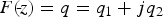 $F(\rlap{\hskip-2pt-} z) = q = q_1 + jq_2 $
, where q
1 defines a constant boundary of the patch and q
2 is tangential to this boundary. Let function F be invertible to an analytic function G of complex variable q, in curvilinear coordinates. This function G(q) may define any patch profile in curvilinear coordinate system.
$F(\rlap{\hskip-2pt-} z) = q = q_1 + jq_2 $
, where q
1 defines a constant boundary of the patch and q
2 is tangential to this boundary. Let function F be invertible to an analytic function G of complex variable q, in curvilinear coordinates. This function G(q) may define any patch profile in curvilinear coordinate system.
Let the circular-shaped patch be represented as G(q) = e q in curvilinear coordinate system. Now the perturbation is applied over the considered profile G(q) to create an arbitrary-shaped patch G 1(q), which may be defined as:
 $$G_1 (q) = e^q \; (1 + \delta X(q)),$$
where X(q) defines the perturbation and δ is used to scale the amount of perturbation. Then the Lame's coefficients H 1 and H 2, which univocally determine the reference coordinate system are calculated for the considered perturbed shape G 1(q) to find the wave solution using (2) and (3).
 $$H_1 = \left \vert {\displaystyle{{\partial G_1 (q)} \over {\partial q_1}}} \right \vert, $$
 $$H_2 = \left \vert {\displaystyle{{\partial G_1 (q)} \over {\partial q_2}}} \right \vert. $$
Consider the perturbation X(q) to be symmetric for degeneracy, to obtain the Lame's coefficients as:
 $$H_1 = H_2 = \left \vert {G^{\prime}_1 (q)} \right \vert = \vert e^q (1 + \delta (X(q) + X{\rm ^{\prime}}(q))).$$
The two-dimensional (2D) Laplacian operator to solve the wave equation in curvilinear coordinates can be expressed as:
 $$\eqalign{\nabla ^2 & = \displaystyle{1 \over {H_1 H_2}} \; \left( {\displaystyle{\partial \over {\partial q_1}} \; \displaystyle{{H_2} \over {H_1}} \; \displaystyle{\partial \over {\partial q_1}} + \displaystyle{\partial \over {\partial q_2}} \; \displaystyle{{H_1} \over {H_2}} \; \displaystyle{\partial \over {\partial q_2}}} \right) \cr & = \vert G^{\prime}_1 (q) \vert ^{ - 2} \; \left( {\displaystyle{{\partial ^2} \over {\partial q_1^2}} + \displaystyle{{\partial ^2} \over {\partial q_2^2}}} \right),}$$
where |G′1(q)|2 = |e q (1 + δ(X(q) + X′(q)))|2.
On further simplification |G′1(q)|2 may be given by:
 $$ \vert G^{\prime}_1 (q) \vert ^2 = e^{2q_1} (1 + 2\delta Re(X(q) + X{\rm ^{\prime}}(q)) + o(\delta ^2 )).$$
Consider small amount of perturbation (δ → 0) for neglecting higher order terms in (6), simplified as:
 $$ \vert G^{\prime}_1 (q) \vert ^2 = e^{2q_1} (1 + 2\delta \eta (q)),$$
where η(q) = Re(X(q) + X′(q)).
Consider a MPA having dielectric substrate of permittivity ε, permeability μ and height d with circular-shaped patch of radius a. It is assumed that the top and bottom surfaces of this patch are perfect electric conductors while the sidewalls are perfect magnetic conductors. The patch profile is then perturbed by a small amount to create an arbitrary-shaped patch. In general, field configuration is obtained by solving the Helmholtz wave equation [Reference Pozar38, Reference Balanis39], therefore this equation is solved in curvilinear coordinates for the considered perturbed patch antenna as:
 $$(\nabla ^2 + h^2 )\psi (q_1, \; q_2 ) = 0,$$
where h is the wave number and ψ is the scalar wave function. The Laplacian operator in (8) may be expanded by using (5) and for simplicity of resultant equation ∂/∂q 1 is replaced by ∂1 and ∂/∂q 2 by ∂2 as given in (9).
 $$(\partial _1^2 + \partial _2^2 + \vert G^{\prime}_1 (q) \vert ^2 h^2 )\psi (q) = 0,$$
|G′1(q)|2 from (7) is substituted into (9) to give:
 $$(\partial _1^2 + \partial _2^2 + h^2 e^{2q_1} (1 + 2\delta \eta (q)))\psi (q) = 0,$$
where ψ(q) and h are the effective scalar wave function and wave number, respectively, expressed as:
 $$\psi (q) = \psi _o (q) + \delta \psi _1 (q) + o(\delta ^2 ),$$
 $$h^2 = h_o^2 + \delta h_1^2 + o(\delta ^2 ).$$
Here, h o = h o [m, n] = α m,n /c is the wave number for the original patch shape and h 1 is the wave number for the perturbed circular patch shape, in which α m,n represents the TM mode of the radiated wave in curvilinear coordinate system and c is the velocity of light. Also, ψ o (q) and ψ 1(q) are the scalar functions of original and perturbed patch shape, respectively.
ψ(q) and h 2 from (11) and (12), are substituted into (10). Then the resultant equation is separated into two parts as perturbed and unperturbed, neglecting the higher order terms. Finally, (10) is converted into the following form:
 $$\eqalign{&(\partial _1^2 + \partial _2^2 + h_o^2 e^{2q_1} )\psi _o (q) + \delta ((\partial _1^2 + \partial _2^2 + h_o^2 e^{2q_1} )\psi _1 (q) \cr & \quad + (h_1^2 e^{2q_1} + 2h_o^2 e^{2q_1} \eta (q))\psi _o (q)) = 0.}$$
Now this wave equation is solved separately for the perturbed and unperturbed parts. Firstly, consider the unperturbed part of (13) as:
 $$[\partial _1^2 + \partial _2^2 + h_o^2 e^{2q_1} ]\psi _o (q) = 0.$$
The above equation is transferred to polar coordinates (r, ϕ, z) for finding the wave solution using e q 1 = r and q 2 = ϕ. The resultant equation is given below:
 $$\left[ {\displaystyle{1 \over r}\displaystyle{\partial \over {\partial r}}r\displaystyle{\partial \over {\partial r}} + \displaystyle{1 \over {r^2}} \displaystyle{{\partial ^2} \over {\partial \phi ^2}} + h_o^2} \right]\; \psi _o (r,\phi ) = 0.$$
Equation (15) may be solved by using the method of separation of variables, and the separated form is given below:
 $$\psi _o (r,\phi ) = R(r).\varphi (\phi ).$$
Now the separated form of ψ o (r, ϕ) is substituted into (15), which then reduces to two one-dimensional (1D) differential equations. The resultant equations are solved to give a complete solution for ψ o as:
 $$\; \psi _o (r,\phi ) = c_1 u_{mn} (r,\phi ) + c_2 v_{mn} (r,\phi ),$$
where c 1, c 2 are the scaling coefficients, u mn and v mn represents the normalized versions of J m (α mn r/a)cos(mϕ) and J m (α mn r/a)sin(mϕ), respectively, in which J m is the mth -order Bessel function. These eigenfunctions are orthogonal with respect to rdrdϕ over 0 ≤ r ≤ a and 0 ≤ ϕ ≤ 2π. Now the perturbed part of (13) is considered to find solution for scalar function ψ 1 as:
 $$\eqalign{&[\partial _1^2 + \partial _2^2 + h_o^2 e^{2q_1} ]\psi _1 (q) + h_1^2 e^{2q_1} \psi _o (q) \cr & \quad + 2h_o^2 e^{2q_1} \eta (q)\psi _o (q) = 0.} $$
Convert the above equation in polar coordinates as earlier:
 $$\eqalign{&\left[ {\displaystyle{1 \over r}\displaystyle{\partial \over {\partial r}}r\displaystyle{\partial \over {\partial r}} + \displaystyle{1 \over {r^2}} \displaystyle{{\partial ^2} \over {\partial \phi ^2}} + h_o^2} \right]\psi _1 (r,\phi ) + h_1^2 \psi _o (r,\phi ) \cr & \quad + 2h_o^2 \eta (r,\theta )\psi _o (r,\theta ) = 0.}$$
Solution of ψ o (r, θ) from (17) is substituted in the above equation, and then the resultant equation is written in Laplacian form as:
 $$\eqalign{(\nabla ^2 + h_o^2 [m,n])\psi _1 (r,\phi ) + h_1^2 (c_1 u_{mn} + c_2 v_{mn} ) \cr + 2h_o^2 [m,n]\eta (r,\phi )(c_1 u_{mn} + c_2 v_{mn} ) = 0,}$$
taking inner product with u kl and v kl of the above equation, resulting in (21) and (22).
 $$\eqalign{&(h_o^2 [m,n] - h_o^2 [k,l])\left\langle {u_{kl}, \; \psi _1} \right\rangle + h_1^2 (c_1 \delta _{mn}. \delta _{ln} ) \cr&+ 2h_o^2 [m,n](c_1 \left\langle {u_{kl}, \; \eta u_{mn}} \right\rangle ) + c_2 \left\langle {u_{kl}, \eta v_{mn}} \right\rangle ) = 0,}$$
 $$\eqalign{&(h_o^2 [m,n] - h_o^2 [k,l])\left\langle {v_{kl}, \; \psi _1} \right\rangle + h_1^2 (c_2 \delta _{mn}. \delta _{kl} ) \cr &+ 2h_o^2 [m,n](c_1 \left\langle {v_{kl}, \eta u_{mn}} \right\rangle + c_2 \left\langle {v_{kl}, \eta v_{mn}} \right\rangle ) = 0.}$$
Rewrite equations (21) and (22) in matrix form for k = m and l = n.
 $$\left[ {\matrix{ {2\beta u_{mn}, \,\eta u_{mn} + h_1^2} & {2u_{mn}, \,\eta u_{mn} \beta} \cr {2\beta v_{mn}, \,\eta v_{mn}} & {2\beta v_{mn}, \, \eta v_{mn} + h_1^2} \cr}} \right]\, \left[ {\matrix{ {c_1} \cr {c_2} \cr}} \right] = 0,$$
where
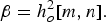 $\beta = h_o^2 [m,n].$
After solving this secular matrix, two perturbed mode eigenvalues for
 $h_1^2 $
are obtained as
$h_1^2 $
are obtained as
 $h_{11}^2 [m,n]$
and
$h_{11}^2 [m,n]$
and
 $h_{12}^2 [m,n]$
, whose corresponding eigenvectors are given below:
$h_{12}^2 [m,n]$
, whose corresponding eigenvectors are given below:
 $$\left[ {\matrix{ {c_{11} [m,n]} \cr {c_{21} [m,n]} \cr}} \right]\; \quad {\rm and}\quad \; \left[ {\matrix{ {c_{12} [m,n]} \cr {c_{22} [m,n]} \cr}} \right].$$
For k ≠ m and l ≠ n, the eigenvectors may be represented as c 1 = c 1i [m, n] and c 2 = c 2i [m, n] for i ∈ (1, 2) to give the wave solutions for perturbed part as:
 $$\left\langle {u_{kl}, \; \psi _1} \right\rangle = \displaystyle{{2h_o^2 [m,n](c_{1i} [m,n]\left\langle {u_{kl}, \; \; \eta u_{mn}} \right\rangle + c_{2i} [m,n]\left\langle {u_{kl}, \; \; \eta u_{mn}} \right\rangle )} \over {(h_o^2 [k,l] - h_o^2 [m,n])}},$$
 $$\left\langle {v_{kl},\, \psi _1} \right\rangle = \displaystyle{\matrix{2h_o^2 [m,n](c_{1i}[m,n]\left\langle {v_{kl},\eta v_{mn}} \right\rangle \hfill \cr + \; c_{2i}[m,n]\left\langle {v_{kl},\, \eta v_{mn}} \right\rangle ) \hfill} \over {(h_o^2 [k,l] - \, h_o^2 [m,n])}}. $$
The generalized solution for the perturbed part ψ 1 is obtained by combining the solutions in (25) and (26).
 $$\psi _{1i} (r,\phi ) = \sum\limits_{(k,l)\; \ne \; (m,n)} {\{ u_{kl} (r,\phi )\left\langle {u_{kl}, \psi _{1i}} \right\rangle + v_{kl} (r,\phi )\left\langle {v_{kl}, \psi _{1i}} \right\rangle \}}. $$
Now, the resultant solutions for perturbed and unperturbed parts are transformed into curvilinear coordinates. This transformation results as:
 $$\psi _o (q_1, q_2 ) = c_1 u_{mn} (q_1, q_2 ) + c_2 v_{mn} (q_1, q_2 ),$$
 $$\eqalign{\delta \psi _{1i} (q_1 , \; q_2 ) & = \delta \sum\limits_{(k,l)\; \ne \; (m,n)} \left\{ u_{kl} (q_1, q_2 )\left\langle {u_{kl} , \; \psi _{1i}} \right\rangle\right.\cr &\quad +\left. v_{kl} (q_1, \; q_2 )\left\langle {v_{kl} , \; \psi _{1i}} \right\rangle \right\}.} $$
Therefore, E-field in the z-direction for the perturbed radiating patch is given below.
 $$\eqalign{E_{z_{mni}} (q_1, q_2 ) &= \psi _o (q_1, q_2 ) + \delta \psi _{1i} (q_1, q_2 ) \cr &= c_{1i} [m,n]u_{mn} (q_1, q_2 ) + c_{2i} [m,n]v_{mn} (q_1, q_2 ) \cr & \quad+ \delta \sum\limits_{(k,l) \ne (m,n)} {\left\{ {\matrix{ {u_{kl} (q_1, q_2 )\left\langle {u_{kl}, \psi _{1i}} \right\rangle \;+} \cr {v_{kl} (q_1, q_2 )\left\langle {v_{kl}, \psi _{1i}} \right\rangle} \cr}} \right\}}.} $$
A generalized form of radiating E-field in the z-direction for arbitrary-shaped MPA may be represented as:
 $$E_z (q_1, q_2, z) = \mathop \sum \limits_{mnpi} E_{z_{mni}} (q_1, q_2 )\sin \left( {\displaystyle{{\pi pz} \over d}} \right)Re\{ Y\}, $$
where m, n, p are the positive integers and Y = α mnpi e (j(h o [m, n]2 + δh 1i [m, n]2 + (π 2 p 2 /d 2 ))1/2 t) , for which α mnpi are complex scalars.
This equation may be used to find E-field pattern for TM mn mode of any arbitrary-shaped patch antenna. Such E-field pattern for any antenna structure may also be obtained by using any commercial software like, FEM-based Ansoft HFSS [40]. However, there is a difference in the way by which these methods are applied on the geometry of the microstrip patch antenna for its field analysis. In the proposed method, the wave equation needs to be solved only within the region of perturbation, and a continuous solution to the potential is obtained in terms of superposition of sine and cosine functions. Also, for better approximation to the true solution higher order perturbation can be applied. Whereas the technique of FEM involves approximation of a continuous potential by discrete vertex potentials in the entire real space, and the grid elements are made smaller for approximating closer to the solution, which increases the overall computation time. This certainly makes the proposed method simpler, accurate and faster in comparison with the FEM-based technique for far-field analysis of arbitrary patch shapes. However, FEM can give more accurate field analysis for patch shapes where there is any change within the boundary such as dissimilar material properties, creation of complex geometry inside the boundary, etc. as this method captures the local regional effects [Reference Madenci and Guven9].
Section III gives the validation of derived E-field equation by numerically analyzing E-field for various patch shapes of microstrip antenna using MATLAB software, and then simulating these arbitrary radiating patch antennas using Ansoft HFSS software for validation.
III. ANTENNA CONFIGURATION AND RESULTS
The derived E-field expression in the previous section can be obtained by evolving the considered shape G 1(q) in curvilinear coordinate system for which the symmetric perturbation X(q) represented as:
 $$X(q) = \mathop \sum \limits_{k = 1}^p c_k q^k, $$
where coefficients c k are used to define the symmetric perturbation. These coefficients can be varied to obtain a particular patch shape for desirable field pattern. After substitution of X(q) from (32) into (1), the considered shape G 1(q) can be expressed as:
 $$G_1 (q) = e^q \left( {1 + \delta \mathop \sum \limits_{k = 1}^p c_k q^k} \right).$$
A regular circular-shaped MPA is considered for validation of E-field expression, i.e. defined in (31). Then the coefficients c k are varied to form two different arbitrary patch shapes for desired directional field patterns. The following subsections show the comparison of theoretical (MATLAB) and simulated (HFSS) results for all the patch shapes, in which the last section also includes the validation of proposed analysis with measured result for one of the created arbitrary patch shapes.
A) Circular patch antenna (ϕ = 0°)
It is noted that C-band has various applications in today's scenario in satellite communication, Wi-Fi devices, weather radar systems etc. and also it offers minimal interference from severe weather conditions resulting in consistent, reliable services for any location. Therefore, this operating band is selected to design a regular circular-shaped MPA to radiate maximally at azimuth angle (xy-plane) ϕ = 0°.
As per the conventional design procedure [Reference Balanis1], initial dimensions of a circular-shaped MPA are calculated for the design frequency of 6 GHz. The antenna layout consists of a circular-shaped patch on grounded dielectric substrate RT/Duroid with relative permittivity ε r of 2.2 and thickness of 0.762 mm, having an overall dimension of 50 mm × 50 mm. Initial simulations are performed to obtain the resonant frequency exactly at 6 GHz, which results into the radius of circular patch a =9.403 mm [Reference Sharma, Upadhyay and Parthasarathy11]. Coaxial probe feeding technique is used to feed the radiating patch since it has the merit of design simplicity through positioning of feed point to adjust the input impedance level [Reference James and Hall7]. Simulated E-field pattern is compared with the theoretical pattern for considered unperturbed circular patch shape G 1(q).
Figure 1(a) shows the physical layout of considered circular-shaped MPA and Fig. 1(b) shows the corresponding theoretical shape G 1(q) with the scaling parameter δ = 0. The structure given in Fig. 1(a) is now simulated to obtain the E-field pattern at elevation angle (yz-plane) θ = 90° for comparison with the theoretical pattern E z (q 1, q 2, z).

Fig. 1. Circular shape (ϕ = 0°). (a) Layout of circular-shaped MPA; (b) theoretical unperturbed circular patch shape.
Figure 2(a) shows the simulated E-field pattern for resonant frequency 6 GHz and Fig. 2(b) gives the comparison of the simulated and theoretical E-field patterns. These results signify that the simulated E-field pattern is similar to the theoretical pattern. Further, it is observed that the maximum and minimum strengths of the simulated E-field are 4.85 (ϕ = 0°) and 0.39 (ϕ = 90°), respectively; however the theoretical values are 5.01 (ϕ = 0°) and 0.36 (ϕ = 90°). These observations validate the theoretical results. It is also noted that the simulated results are broadside symmetric for the considered circular MPA.

Fig. 2. Radiation patterns for circular-shaped MPA (ϕ = 0°). (a) Simulated E-field pattern for −90° < ϕ <90° (clockwise), (b) comparison of the simulated and theoretical E-field patterns for −90°< ϕ <90° (clockwise).
Figure 3 shows the other characteristics for circular MPA as return loss, gain versus ϕ, gain versus frequency and CPL. From Fig. 3(a), it is observed that the considered radiating patch resonates at 6 GHz with return loss −23.14 dB, having the impedance bandwidth of 120 MHz. Further, Fig. 3(b) shows the value of broadside gain as 7.68 dB (ϕ = 0°) at 6 GHz; however Fig. 3(c) gives gain of 7.70 dB (ϕ = 0°) at 6.09 GHz. The field components E θ and E ϕ are also traced at θ = 90° in Fig. 3(d) to calculate CPL of −53 dB.

Fig. 3. Characteristics of circular MPA (ϕ = 0°). (a) Return loss, (b) gain versus ϕ, (c) gain versus frequency, (d) cross-polarization level.
B) Arbitrary-shaped antenna (ϕ = −45°)
The coefficients of the patch shape G 1(q) are varied to perturb the considered circular shape of patch for achieving the desired radiation characteristics. Therefore, a new arbitrary patch shape is evolved, i.e. perturbed at the circumference of circular patch, which has the maximum field strength directed at ϕ = −45°. Figure 4(a) shows the developed theoretical shape G 1 (q) with δ = 0.029 and Fig. 4(b) shows the corresponding layout of proposed arbitrary shape (ϕ = −45°), preserving the structure configuration of original circular MPA.

Fig. 4. Arbitrary shape (ϕ = −45°). (a) Theoretical arbitrary-shaped patch, (b) layout of arbitrary-shaped MPA.
The proposed arbitrary-shaped MPA (ϕ = −45°) is simulated, then it is observed that the resonant frequency shifted to 5.18 GHz owing to change in effective dimensions of considered patch. Figure 5(a) shows the simulated E-field pattern (θ = 90°) and Fig. 5(b) shows the comparison of theoretical and simulated E-field patterns. It clears that the simulated field pattern is comparable with the theoretical pattern. Further, it is observed that the direction of maximum field strength rotates anticlockwise by 45° as compared with that of circular MPA, the maximum strengths of simulated and theoretical E-field are 4.24 and 4.22 at ϕ = −45° respectively, however the minimum strengths are 1.76 (ϕ = 60°) and 1.83 (ϕ = 10°).

Fig. 5. Radiation patterns for arbitrary-shaped MPA (ϕ = −45°). (a) Simulated E-field pattern for − 120° < ϕ < 60° (clockwise), (b) comparison of the theoretical and simulated E-field patterns for −120° < ϕ < 60° (clockwise).
Figure 6 shows the other antenna characteristics for arbitrary-shaped MPA (ϕ = −45°) as return loss, gain versus ϕ, gain versus frequency and CPL. Figure 6(a) clears that the considered radiating patch resonates at 5.18 GHz with return loss −24.82 dB, having the improved impedance bandwidth of 230 MHz as compared with that of circular MPA. Further, Fig. 6(b) shows the gain as 6.87 dB (ϕ = −45°) at 5.18 GHz; however Fig. 6(c) gives gain of 7.13 dB (ϕ = −45°) at 5.15 GHz. From Fig. 6(d), it is clear that the CPL is reduced to −7.40 dB. Therefore, the proposed structure has trade-off between the impedance bandwidth and CPL characteristics. Circular polarization is also observed in Fig. 7 for the proposed radiating structure with axial ratio of 0.32 dB at resonant frequency.

Fig. 6. Characteristics of arbitrary-shaped MPA (ϕ = −45°). (a) Return loss, (b) gain versus ϕ, (c) gain versus frequency, (d) cross-polarization level.

Fig. 7. Axial ratio of arbitrary-shaped MPA (ϕ = −45°).
C) Arbitrary-shaped antenna (ϕ = −180°)
The coefficients for the patch shape G 1(q) are again varied for achieving maximum E-field strength along direction ϕ = −180°. This variation perturbs the circular shape to new arbitrary shape with δ = 0.052, i.e. given in Fig. 8(a). Further, Fig. 8(b) shows the corresponding layout of proposed arbitrary shape (ϕ = −180°), preserving the structure configuration of original circular MPA. This shape is also fabricated to validate the proposed technique, i.e. creating arbitrary-shaped MPAs for the desired field pattern, with measured results. The fabricated model is shown in Fig. 8(c).

Fig. 8. Arbitrary shape (ϕ = −180°). (a) Theoretical arbitrary-shaped patch, (b) layout of arbitrary-shaped MPA, (c) prototype of arbitrary-shaped patch antenna.
The proposed arbitrary-shaped MPA (ϕ = −180°) is simulated, and then it is observed that the resonant frequency shifted to 6.34 GHz due to the variation in effective dimensions of considered patch. Figure 9(a) shows the simulated E-field pattern (θ = 90°) and Fig. 9(b) shows the comparison of theoretical, simulated, and measured E-field patterns. These radiation results clear that the measured and simulated pattern appears to be same as the theoretical pattern. It is also observed that the direction of maximum field strength rotates anticlockwise by 180° as compared with that of circular MPA. Further, it is noted that the maximum strengths of measured, simulated and theoretical E-field are 4.82, 4.96, and 4.87 at ϕ = −180°; respectively; however, the minimum strengths are 1.48, 0.96, and 1.00 at ϕ = 90°.

Fig. 9. Radiation patterns for arbitrary-shaped MPA (ϕ = −180°). (a) Simulated E-field pattern for − 90° < ϕ < 90° (anticlockwise), (b) comparison of theoretical and simulated E-field patterns for −90° < ϕ < 90° (anticlockwise).
Figure 10 shows the other characteristics for arbitrary-shaped MPA (ϕ = −180°) as return loss, gain versus ϕ, gain versus frequency and CPL. It is observed from Fig. 10(a) that this patch antenna resonates at 6.34 GHz with return loss −12.16 dB, having the impedance bandwidth of 40 MHz as compared with that of original circular MPA. Further, Fig. 10(b) clears that the gain is 7.36 dB (ϕ = −180°) at 6.34 GHz; however, Fig. 10(c) gives gain of 7.37 dB (ϕ = −180°) at 6.35 GHz. Figure 10(d) shows that the CPL is reduced to −44.31 dB. These observations may conclude that the theoretical E-field pattern for any patch shape holds in good agreement with the simulated HFSS results.

Fig. 10. Characteristics of arbitrary-shaped MPA (ϕ = −180°). (a) Return loss, (b) gain versus ϕ, (c) gain versus frequency, (d) cross-polarization level.
IV. CONCLUSION
Field analysis of an arbitrary-shaped MPA is evolved by deriving the E-field expression based on the concept of perturbation theory. Change in the geometry of a radiating patch varies the impedance and radiation characteristics such as gain, bandwidth, CPL, direction of radiation, etc. A mathematical perturbed shape is defined in the curvilinear coordinate system to create different arbitrary patch shapes for the desired radiation pattern. Initially, a regular circular-shaped MPA is designed for broadside radiation pattern (ϕ = 0°) to validate the evolved field analysis. Further, this analysis is used to create two arbitrary-shaped patch antennas, which radiate maximally in the directions of ϕ = −45° and − 180°. The simulated results show that the designed MPA (ϕ = −45°) has improved bandwidth of 230 MHz with additional characteristic of circular polarization at resonant frequency, and other designed MPA (ϕ = −180°) radiates exactly in opposite direction to that of circular MPA, preserving its radiation characteristics at the cost of impedance bandwidth. The method presented in this paper is simple, accurate, adaptable, fast, and will serve as a useful tool in the design and analysis of MPA for pattern specific applications.
ACKNOWLEDGEMENTS
The authors are highly grateful to the Director of NSIT, Delhi, India, for his constant encouragement and provision of facilities for this research work. Also, we are thankful to the anonymous reviewers for their constructive comments, which helped us improve the manuscript.
 Karishma Sharma received her B.Tech. degree in Electronics and Communication Engineering in 2011 from GGSIPU, Delhi, India. She was awarded gold medal and an exemplary performer in her M.Tech., from GGSIPU, Delhi, India in 2013. She is currently pursuing her Ph.D. in the area of Design and Analysis of Microstrip patch antenna from Netaji Subhas Institute of Technology, Delhi University, Delhi, India. Her research interests include antenna design and its analysis, applied electromagnetic theory, metamaterials, digital, and wireless communication.
 Dharmendra K. Upadhyay holds Bachelor of Engineering in Electronics and Communication Engineering from Kumaon University, Nainital, India and Master of Technology in Communication and Information Systems from Aligarh Muslim University, Aligarh, UP, India. He obtained his Ph.D. from Uttrakhand Technical University, Dehradun, Uttrakhand, India in 2013. Presently, he is associated with Netaji Subhas Institute of Technology, Delhi, India, as a Professor in the Division of Electronics and Communication Engineering. He has published several papers in various International Journals. He is a life member of ISTE. His research interests include microstrip patch antenna designs, microwave filters, and digital signal processing.
 Harish Parthasarathy received the Bachelor's degree in 1990 from the Indian Institute of Technology, Kanpur, India and Ph.D. in 1994 from the Indian Institute of Technology, Delhi, India, both in Electrical Engineering. He is currently working as a Professor at Netaji Subhas Institute of Technology, Delhi University, Delhi, India. He is an eminent academician and a great researcher, and has authored more than 100 research articles in various international journals of repute. His research interests include the areas of electromagnetic theory, antennas, quantum mechanics, circuits and systems, signal processing, and stochastic nonlinear filters.


