


I. INTRODUCTION
Radar receivers must receive very low-power signals and discern them from the noise. Radar received signal strength is related to the transmitted power by the inverse of the distance raised to the fourth power, whereas communication received signal strength is related to transmitted power by the inverse of the distance squared. Low-noise amplifiers (LNA) are finding significant contemporary application in radar receivers, including automotive radar at 75–77 GHz [Reference Eye and Allen1, Reference Hartmann, Wagner, Seemann, Platz and Weigel2], X-band radar transmit-receive modules near 10 GHz [Reference Kuo, Liang, Cressler and Mitchell3], and near-space radar applications [Reference Kuo4]. Dawood and Narayanan demonstrate that the output of the radar correlation operation (used for signal identification) is related to the signal-to-noise ratio at the input to the correlator [Reference Dawood and Narayanan5]. Since noise figure is a key issue in LNA design, this means that the front-end LNA plays a significant role in the back-end detection capability of a radar system.
Both the noise figure and available gain of an LNA are functions of the source reflection coefficient Γ s [Reference Fukui6]. The designer must decide between choosing Γ s = Γ opt for minimum noise figure, selecting Γ s for optimum gain, or finding a compromise. In many cases, a compromise is necessary, as it is desired to find the highest possible value of available gain G A while insuring that the noise figure F is below the design limitations.
The literature shows work in optimization and estimation of constrained optima, but, to our knowledge, does not present an analytical solution for the optimal design value of Γ s . Fukui demonstrates the plotting of noise figure and gain circles on the Smith chart for design purposes [Reference Fukui6]. Nieuwoldt et al. describe a Pareto optimization approach using Sequential Quadratic Programming and the Normal Boundary Intersection Method; their optimization is applied to objective functions that include noise figure, gain, and power dissipation under constraints of output and input impedance matching networks and also limitations on component values [Reference Nieuwoldt, Ragheb and Massoud7]. The same group demonstrates a wideband LNA synthesis approach for multiple performance measures in [Reference Nieuwoudt, Ragheb and Massoud8]. Nguyen et al. compare four different LNA optimization techniques used in CMOS designs, including a technique that uses source degeneration to try to make the optimum impedances for noise figure and input voltage standing-wave-ratio similar [Reference Nguyen, Kim, Ihm, Yang and Lee9]. For Si and Ge transistors, Fukui provides expressions for noise figure based on a small-signal model representation of the device, and also investigates the optimal current [Reference Fukui10]. He also discusses the optimization of gate length in GaAs metal semiconductor field-effect transistors [Reference Fukui11]. Hashemi and Hajimiri describe gain and noise figure design for concurrent multiband LNAs based on the equivalent circuit model and noise equivalent circuit for the active device [Reference Hashemi and Hajimiri12].
Niu et al. demonstrate how designing for low noise figure affects the potential to achieve high power gain [Reference Niu, Cressler, Zhang, Joseph and Harame13]. Gonzalez describes design issues for noise and gain in his book on linear transistor amplifier design, and demonstrates optimization for different noise and gain requirements by drawing a line from the optimum gain source impedance to the optimum noise figure source impedance in the Smith chart [Reference Gonzalez14] and calculating variations of gain and noise figure along the line. While many have used rule-of-thumb approximations, the present paper shows from the theory that the Pareto trade-off need not be approximated, but can be directly obtained from the S-parameters and noise parameters.
This paper describes how to directly find the source reflection coefficient providing the largest available gain while meeting noise figure constraints, or the source reflection coefficient providing the smallest noise figure while meeting available gain constraints. This is a constrained optimization problem based on two convex sets (gain and noise figure). Pareto optimization involves finding a tradeoff between two conflicting objectives. Miettenen discusses multiple-objective optimization and provides examples from economics, mathematics, and engineering [Reference Miettinen15]. A similar situation requiring the use of Pareto analysis is the optimization of load reflection coefficient for linearity and efficiency [Reference Baylis16–Reference Fellows, Baylis, Martin, Cohen and Marks19] in power amplifiers. However, the power amplifier problem is a nonlinear optimization that must be performed sequentially. For source impedance optimization in LNAs, linear behavior is assumed, allowing the Pareto optimum to be found analytically using the S-parameters and noise parameters.
This paper presents theory that can be applied in many various ways in LNA design and optimization. One particularly useful application is reconfigurable LNAs. In a reconfigurable LNA, many of the parameters involved in a design are fixed, such as bias, source inductance, stabilization networks, and other parameters. However, the source impedance may be constructed from reconfigurable elements to allow tuning around the Smith chart in real-time. In such case, the approach presented in this paper is useful in finding the value of Γ s providing maximum gain under noise figure constraints or providing minimum noise figure under gain constraints. The requirements may change in mobile systems due to different expected signal-to-noise ratio of the input signal and requirements for signal-to-noise ratio of the RF front end.
Section II provides a theoretical description of the gain versus noise-figure tradeoff and derives equations to be solved to find the optimum noise figure given available-gain constraints or optimum available gain given noise-figure constraints. Section III presents examples of how this technique can be used for design in cases where the device is unconditionally stable and potentially unstable. Section IV provides conclusions regarding the work.
II. GAIN AND NOISE FIGURE
The locus of points providing a constant available gain G A in a linear amplifier is a circle in the Smith chart [Reference Gonzalez14]. In addition, the locus of points providing a constant specified noise figure N i is also a circle in the Smith chart [Reference Gonzalez14]. As such, Fig. 1 depicts the situation in which circles of constant G A and N i are drawn in the Smith chart. The equations for the center C a and radius r a of a given G A circle are given in terms of the value of the normalized available gain, g a = G A /|S 21|2, as follows [Reference Gonzalez14]:
 $${C_a} = \displaystyle{{{g_a}C_1^{\ast}} \over {1 + {g_a}({{\left\vert {{S_{11}}} \right\vert} ^2} - {{\left\vert \Delta \right\vert} ^2})}},$$
 $${r_a} = \displaystyle{{{{\left[ {1 - 2K\left\vert {{S_{12}}{S_{21}}} \right\vert {g_a} + {{\left\vert {{S_{12}}{S_{21}}} \right\vert} ^2}g_a^2} \right]}^{1/2}}} \over {\left\vert {1 + {g_a}({{\left\vert {{S_{11}}} \right\vert} ^2} - {{\left\vert \Delta \right\vert} ^2})} \right\vert}}, $$
where Δ = S
11
S
22 − S
12
S
21, K = (1 − |S
11|2 − |S
22|2 + |Δ|2)/(2|S
12
S
21|), and
 ${C_1} = {S_{11}} - \Delta S_{22}^{\ast} $
.
${C_1} = {S_{11}} - \Delta S_{22}^{\ast} $
.
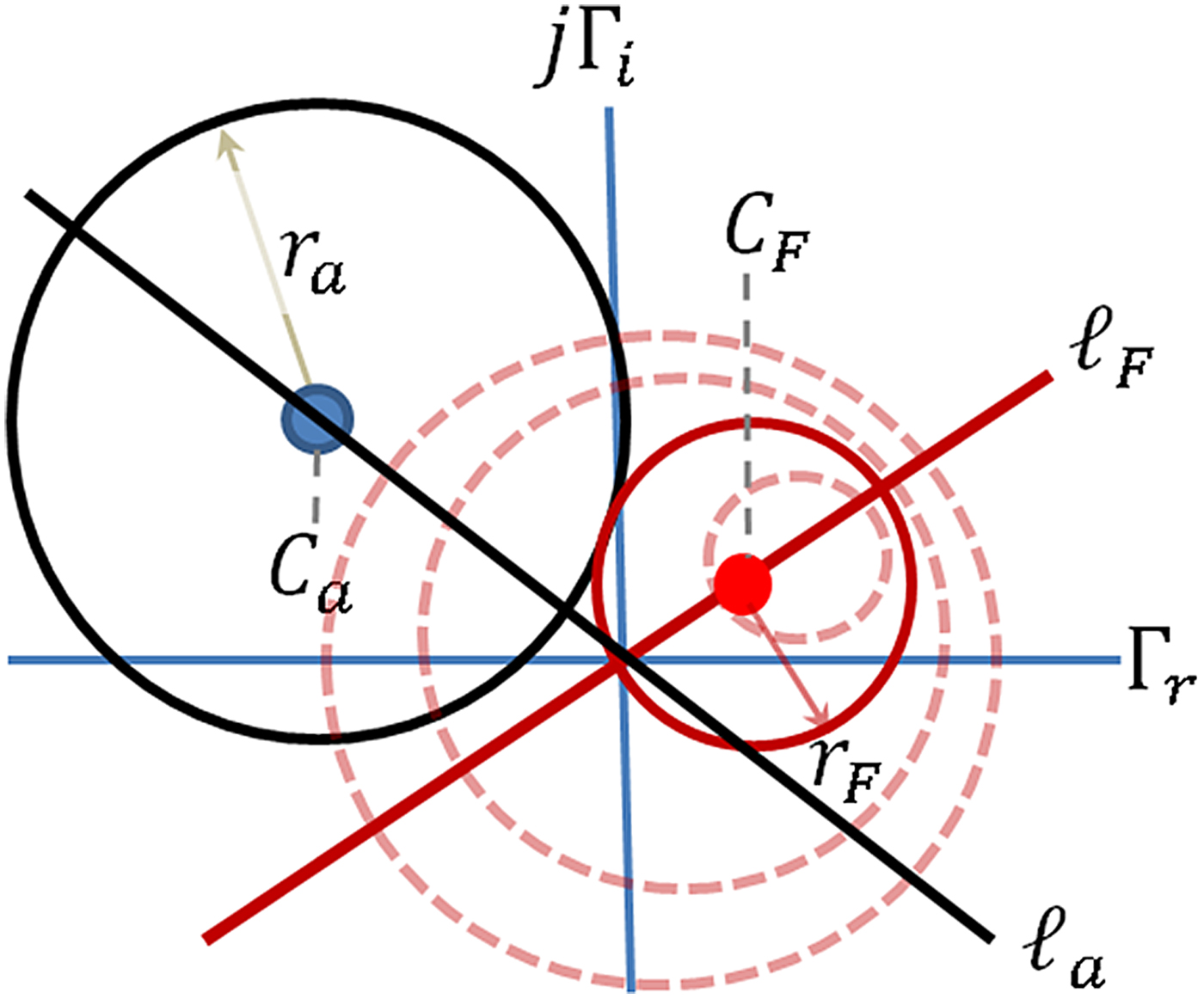
Fig. 1. Circles of constant gain and noise figure on the complex Γ s plane (the Smith chart).
Additionally, the center and radius of circles of constant noise figure are given in terms of the noise measure
 $${N_i} = \displaystyle{{{F_i} - {F_{min}}\;} \over {4{r_n}}}{\left\vert {1 + {{\Gamma} _{opt}}} \right\vert ^2},$$
where F i is the noise figure and F min , Γ opt , and r n are the noise parameters of the device representing the minimum noise figure, optimum reflection coefficient for noise figure, and normalized noise resistance, respectively. The equations for the center and radius of the noise figure circles, based on the noise measure, are given as follows [Reference Gonzalez14]:
 $${C_F} = \displaystyle{{{{\Gamma} _{opt}}} \over {1 + {N_i}}},$$
 $${r_F} = \displaystyle{1 \over {1 + {N_i}}}\sqrt {N_i^2 + {N_i}\left( {1 - {{\left\vert {{{\Gamma} _{opt}}} \right\vert} ^2}} \right)} \;. $$
Equations (1) and (4) show that both the gain and noise circles are centered along straight lines emanating from the origin of the complex Γ s plane, as shown in Fig. 1.
A point in the Γ s plane is on the locus of Pareto optimum points if and only if one of the F i circles is tangent to one of the G A circles at that point. For this to be true, the distance between the center of the G A circle and the center of the F circle must equal the sum of the radii of the circles. The distance between the circle centers, from equations (1) and (4), is given by
 $${D} = {\left\vert {{C_a} - {C_F}} \right\vert} = {\left\vert {\displaystyle{{{g_a}C_1^{\ast}} \over {1 + A{g_a}}} - \displaystyle{{{{\it \Gamma} _{opt}}} \over {1 + {N_i}}}\;} \right\vert}, $$
where A = |S 11|2 − |Δ|2. Optimality occurs when D = r a + r F , or
 $${\left\vert {\displaystyle{{{g_a}C_1^{\ast}} \over {1 + A{g_a}}} - \displaystyle{{{{\Gamma} _{opt}}} \over {1 + {N_i}}}\;} \right\vert} = \displaystyle{{\sqrt {1 - a{g_a} - bg_a^2}} \over {\left\vert {1 + A{g_a}} \right\vert}} + \displaystyle{{\sqrt {N_i^2 + c{N_i}}} \over {1 + {N_i}}}, $$
using equations (2) and (5), where a = 2K|S
11
S
21|, b = −|S
12
S
21|2, and
 $c = 1 - {\left\vert {{{\Gamma} _{opt}}} \right\vert^2}$
. Multiplying both sides of (7) by (1 + N
i
)|1 + Ag
a
| and squaring both sides gives
$c = 1 - {\left\vert {{{\Gamma} _{opt}}} \right\vert^2}$
. Multiplying both sides of (7) by (1 + N
i
)|1 + Ag
a
| and squaring both sides gives
 $$\eqalign{& {\left\vert {s\left( {1 + {N_i}} \right)\,{g_a}C_1^{\ast} - \left\vert {1 + A{g_a}} \right\vert {{\Gamma} _{opt}}} \right\vert ^2} \cr & \quad= {\left[ {\left( {1 + {N_i}} \right)\sqrt {1 - a{g_a} - bg_a^2} + {{\left\vert {1 + A{g_a}} \right\vert}} \sqrt {N_i^2 + c{N_i}}} \right]^2},} $$
where s = sign(1 + Ag a ) = ±1. Since, for any complex numbers z 1 and z 2,
 $${\left\vert {{z_1} - {z_2}} \right\vert ^2} = {\left\vert {{z_1}} \right\vert ^2} + {\left\vert {{z_2}} \right\vert ^2} - 2{\rm \Re} {\rm \;} {z_1}\; z_2^{\ast}. $$
Equation (8) can be written as
 $$\eqalign{&{(1 + {N_i})^2}g_a^2\vert {C_1}{\vert ^2} +\vert 1 + A{g_a}{\vert ^2}\vert {{\it \Gamma} _{opt}}{\vert ^2} \cr & \quad - 2s{g_a}\vert 1 + A{g_a}\vert (1 + {N_i})\Re ({C_1}{{\Gamma} _{opt}}) \cr & = {(1 + {N_i})^2}(1 - a{g_a} - bg_a^2 ) +\vert 1 + A{g_a}{\vert ^2}(N_i^2 + c{N_i}) \cr & \quad+ 2(1 + {N_i})\vert 1 + A{g_a}\vert \sqrt {(1 - a{g_a} - bg_a^2 )(N_i^2 + c{N_i}).}} $$
There are two cases of interest for LNA design: (1) optimization of the noise measure N i while bounding the gain g a and (2) optimization of g a while bounding N i .
Case 1: bound g a and optimize Ni .
A lower bound is placed on the normalized available gain g a , and under this constraint, it is desired to minimize the noise figure F i and hence the noise measure N i . With g a as a fixed value, an expression in terms of N i can be developed. Equation (10) can be rewritten as a fourth-order polynomial in N i :
 $${A_4}N_i^4 + {A_3}N_i^3 + {A_2}N_i^2 + {A_1}N_i + {A_0} = 0,\; $$
where
 $${A_4} = {\left( {\alpha + \gamma} \right)^2} + 4\gamma \delta, $$
 $${A_3} = 2\left( {\alpha + \gamma} \right){(2\alpha - \beta + c\gamma )_\;} + \; 4\gamma \; \delta \left( {2 + c} \right),$$
 $$\eqalign{{A_2} & = 2\left( {\alpha - \beta - \gamma {{\left\vert {{{\Gamma} _{opt}}} \right\vert} ^2}} \right)\left( {\alpha + \gamma} \right) \cr & \quad +(2\alpha - \beta + c\gamma )\; ^{2} + 4\gamma \; \delta \left( {1 + 2c} \right),} $$
 $${A_1} = 2(2\alpha - \beta + c\gamma ){\left( {\alpha - \beta - \gamma {{\left\vert {{{\Gamma} _{opt}}} \right\vert} ^2}} \right)_\;} + 4\gamma \delta c,$$
 $${A_0} = {\left( {\alpha - \beta - \gamma {{\left\vert {{{\Gamma} _{opt}}} \right\vert} ^2}} \right)^2} + 4\gamma \delta, $$
 $$\alpha = g_a^2 \; {\left\vert {C_1} \right\vert ^2} - \delta, $$
 $$\beta = 2s{g_a}\left\vert {1 + A{g_a}} \right\vert \Re \; \left( {C_1 {{\Gamma} _{opt}}} \right),$$
 $$\gamma = - {\left\vert {1 + A{g_a}} \right\vert ^2},$$
 $${\delta = 1 - a{g_a} - bg_a^2}. $$
Case 2: bound N i and optimize ga.
Because s 2 = 1, |1 + Ag a | = s(1 + Ag a ), if N i is assigned a fixed, limiting value, equation (10) can be rewritten (using the observation that s 2 = 1) as a fourth-order polynomial in g a :
 $${{B_4}g_a^4 + {B_3}g_a^3 + {B_2}g_a^2 + {B_1}g_a + {B_0} = 0}, $$
where
 $${B_4} = - b\nu {A^2} - {\lambda ^2}, $$
 $${{B_3} = - a{A^2}v - 2bAv - 2\lambda \varphi}, $$
 $${{B_2} = {A^2}v - 2aAv - bv - 2\theta \lambda - {\varphi ^2}}, $$
 $${{B_1} = 2Av - av - 2\theta \varphi}, $$
 $${{B_0} = v - {\theta ^2}},$$
 $$\nu = 4{\left( {1 + {N_i}} \right)^2}\left( {N_i^2 + c{N_i}} \right),\; $$
 $${\lambda = {\left( {1 + {N_i}} \right)^2}\left( {{{\left\vert {C_1} \right\vert} ^2} + b} \right) + {A^2}\; \xi - 2A\eta}, $$
 $${\varphi = a{\left( {1 + {N_i}} \right)^2} + 2A\xi - 2\eta}, $$
 $${\theta = \xi - {\left( {1 + {N_i}} \right)^2}}, $$
 $${\xi = {\left\vert {{\Gamma _{opt}}} \right\vert ^2} - N_i^2 - c{N_i}}, $$
 $$\eta = \left( {1 + {N_i}} \right)\Re \left( {C_1 {\Gamma _{opt}}} \right).\; $$
In both Case 1 and Case 2, a fourth-order polynomial can be solved for N i (Case 1) or g a (Case 2) by using typical fourth-order polynomial solution techniques. Following the solution to the polynomial, both N i and g a will be known. This means that the center and radius of both the available gain circle corresponding to the value of g a and the noise figure circle corresponding to the value of N i can be calculated using equations (1), (2), (4), and (5). A complex number of magnitude 1 and phase equal to the angle in the complex plane with the Re(Γ s ) axis formed by a straight line from C F to C a is given by μ:
 $$\mu = \displaystyle{{{C_a} - {C_F}} \over {\left\vert {{C_a} - {C_F}} \right\vert}}, $$
where C
a
and C
F
are defined by (4) and (5). μ (in the complex plane) is analogous to a unit vector from vector theory. μ can be used to find the constrained optimum source reflection coefficient
 ${{{\tilde{\Gamma} _{\rm s}}}}$
:
${{{\tilde{\Gamma} _{\rm s}}}}$
:
 $${{\rm \tilde \Gamma} _{\rm s}} = {C_F} + {r_F}\mu.$$
III. LNA PARETO OPTIMIZATION EXAMPLES
Two design optimization examples are provided where a limitation on the noise figure is placed, and it is desired to find the source reflection coefficient Γ s providing the maximum value of G A while meeting given noise figure limitations. For brevity we have chosen to focus on this case (Case 2 from Section II), but Case 1 (finding the minimum value of F i while meeting G A limitations) follows dual procedures.
Example 1: unconditionally stable device
Consider a device whose S-parameters and noise parameters are given by the following: S
11 = 0.642e
−j110°, S
12 = 0.02e
j45°, S
21 = 4.54e
−j126°, S
22 = 0.33e
−j82.1°, F
min
= 1.3 dB,
 ${{\Gamma} _{opt}} = 0.43{e^{j175{{\tf="pi1" 8}}}} $
, and R
n
= 9.3 Ω. It is desired to design a LNA with the available gain as high as possible while possessing a noise figure no greater than 2 dB.
${{\Gamma} _{opt}} = 0.43{e^{j175{{\tf="pi1" 8}}}} $
, and R
n
= 9.3 Ω. It is desired to design a LNA with the available gain as high as possible while possessing a noise figure no greater than 2 dB.
Stability metrics are calculated as follows: |Δ| = 0.259 and K = 3.006. Because K > 1 and |Δ| <1, this device is unconditionally stable. It is desired to limit the noise figure to F i = 2 dB, giving N i = 0.104. The quartic polynomial in (21) becomes
 $$- 0.099g_a^4 - 0.36g_a^3 + 0.321g_a^2 + 1.256g_a - 0.81 = 0.$$
This polynomial has four roots that can easily be found by a numerical solver: g
a
= −2.898, −2.898, 0.627, 1.546. Since it is the largest constrained value of g
a
that is sought, the root chosen is g
a
= 1.546, resulting in G
A
= 15.033 dB. Solving (33) and (34) gives μ = 1e
j66.47°and
 ${\tilde{{{\Gamma} _{\rm s}}}} = 0.401{e^{j133.522{\tf="pi1" 8}}}. $
At
${\tilde{{{\Gamma} _{\rm s}}}} = 0.401{e^{j133.522{\tf="pi1" 8}}}. $
At
 ${{\tilde{\Gamma _s}}}$
the maximum constrained value of available gain while maintaining the noise figure less than or equal to 2 dB, G
A
= 15.033 dB, is obtained. Figure 2 shows the Pareto optimum value of source reflection coefficient, along with the associated available-gain and noise-figure circles.
${{\tilde{\Gamma _s}}}$
the maximum constrained value of available gain while maintaining the noise figure less than or equal to 2 dB, G
A
= 15.033 dB, is obtained. Figure 2 shows the Pareto optimum value of source reflection coefficient, along with the associated available-gain and noise-figure circles.
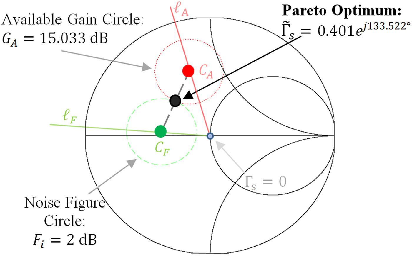
Fig. 2. Pareto optimum source reflection coefficient for Example 1 providing maximum constrained available gain with noise figure less than or equal to 2 dB, plotted with the associated noise figure (2 dB) and available gain circles (15.033 dB).
The collection of Pareto optimum reflection coefficients for different limiting values of noise figure can be plotted in the Γ s Smith chart as in Fig. 3. This locus is generated by solving the Pareto optimization problem for multiple limiting values of noise figure spanning from F min until the maximum-gain reflection coefficient Γ Ms is reached (in the unconditionally stable case). This collection of points provides optimal trade-off values between gain and noise figure. The same collection of points is obtained by solving the Pareto optimization problem for multiple limiting values of g a . The Pareto optimum locus extends from Γ opt , the reflection coefficient providing optimum noise figure, to Γ Ms , the reflection coefficient providing maximum available gain. While the literature often suggests the “rule-of-thumb” method of drawing a straight line between the gain and noise figure optima to perform Pareto designs [Reference Gonzalez14], the Pareto optimum locus is generally not a straight line between the points, but rather a curve connecting them.

Fig. 3. Pareto optimum locus for Example 1: the collection of Γ s points providing optimum available gain for different bounded noise figure values. Note that the Pareto locus is not a straight line.
Figure 4 shows the Pareto front. The Pareto front is a plot of the gain-versus-noise tradeoff for the values of Γ s on the Pareto optimum locus, and it shows the maximum values of G A that can be obtained under different limiting values of F i . The plot begins at the minimum noise figure F i = F min = 1.3 dB and ends at the maximum available gain, which occurs at a simultaneous conjugate match for the device [Reference Gonzalez14]:
 $${G_{A,max}} = \displaystyle{{\left\vert {{S_{21}}} \right\vert} \over {\left\vert {{S_{12}}} \right\vert}} \left( {K - \sqrt {{K^2} - 1}} \right) = 15.895\; dB$$

Fig. 4. Pareto front for Example 1: values of available gain G A for different limiting values of noise figure F i .
Example 2: potentially unstable device
Consider a device whose S-parameters and noise parameters are given as follows: S
11 = 0.6e
j26°, S
12 = 0.07e
j162°, S
21 = 5.14e
−j34°, S
22 = 0.45e
j72.5°, F
min
= 1.8 dB,
 ${{\Gamma} _{opt}} = 0.31{e^{j80{\tf="pi1" 8}}} $
, and R
n
= 5.4 Ω. It is desired to design a LNA with a noise figure less than or equal to 2 dB and the largest available gain under this constraint.
${{\Gamma} _{opt}} = 0.31{e^{j80{\tf="pi1" 8}}} $
, and R
n
= 5.4 Ω. It is desired to design a LNA with a noise figure less than or equal to 2 dB and the largest available gain under this constraint.
The stability metrics of the device are calculated to be |Δ| = 0.182 and K = 0.654. Because K < 1, the device is potentially unstable [Reference Gonzalez14]. This does not significantly affect the design procedure, but the stability circle should be drawn and care should be taken that the Pareto optimum is in the stable region on the Smith chart.
For reference in choosing the gain, the maximum stable gain is calculated as in [Reference Gonzalez14]: G MSG = 18.659 dB. It is desired to limit the noise figure to 2 dB, resulting in N i = 0.199 from (3). Finding a, b, and c, and then using equations (21) through (32) gives the quartic polynomial of (20) for solution:
 $$- 0.16g_a^4 - 0.614g_a^3 + 0.617g_a^2 + 2.664g_a - 1.174 = 0$$
Solving this polynomial numerically with a mathematical software package results in four roots: −3.061, −3.06, 0.419, and 1.868. The largest of the roots is the root that will be used: g
a
= 1.868, corresponding to G
A
= 16.933 dB. Using (33) and (34) gives μ = 1e
−j49.4° and
 ${{\rm \tilde \Gamma} _{\rm s}} = 0.302{e^{ - j7.92{\tf="pi1" 8}}} $
.
${{\rm \tilde \Gamma} _{\rm s}} = 0.302{e^{ - j7.92{\tf="pi1" 8}}} $
.
This choice of reflection coefficient provides F i = 2 dB and G A = 16.933 dB. This gain is less than the maximum stable gain, which serves as an informal figure of merit indicating a comfortable level of gain that can be accomplished without too closely approaching instability. Figure 5 shows the Pareto optimum source reflection coefficient along with its associated available gain and noise figure circles. The input stability circle is also shown on this plot. Because |S 22| <1, the center of the Smith chart is in the stable region [Reference Gonzalez14], so the identified Pareto optimum source reflection coefficient will provide stable operation. Figure 6 shows the Pareto optimum locus for this device. Because the device is potentially unstable, the Pareto optimum locus approaches the unstable region rather than a stable gain optimum. Figure 7 shows the Pareto front.
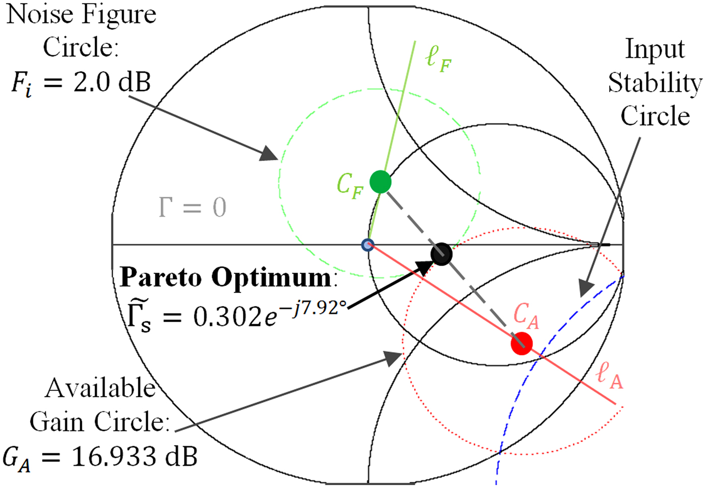
Fig. 5. Pareto optimum source reflection coefficient for Example 2 providing maximum constrained available gain with noise figure less than or equal to 2.0 dB, plotted with the associated noise figure (2.0 dB) and available-gain (16.933 dB) circles. The stability circle is also shown, and it is apparent that the Pareto optimum solution is in the stable region.
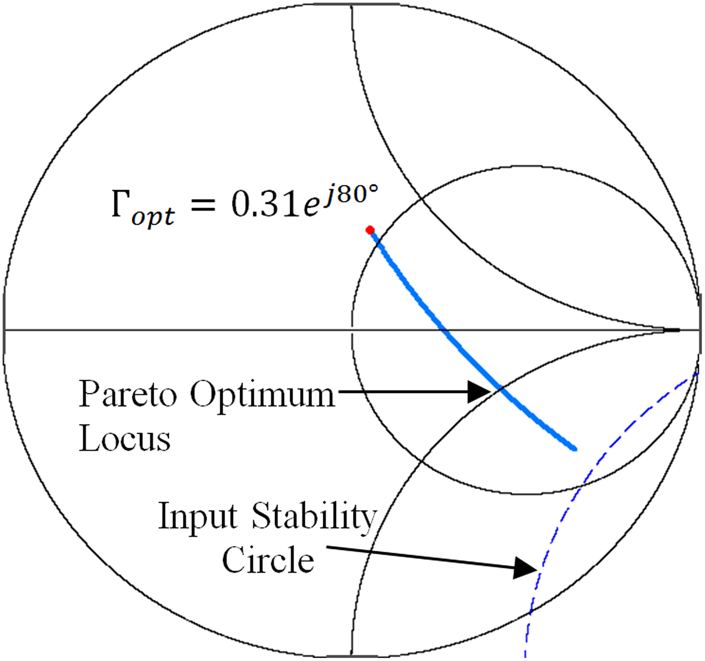
Fig. 6. Pareto optimum locus for Example 2: the Pareto optimum locus goes between the optimum noise figure termination and the stability circle for this potentially unstable device. Note that the Pareto locus is not a straight line.
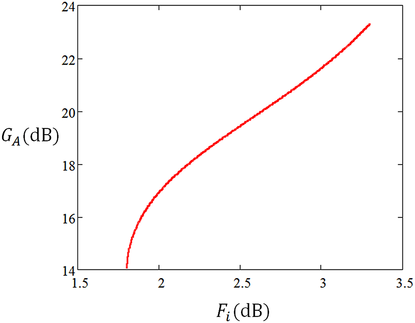
Fig. 7. Pareto front for Example 2: values of available gain G A for different limiting values of noise figure F i .
While the constrained optimum
 $\tilde{{{{\Gamma} _{\rm s}}}} = 0.302{e^{ - j7.92{\tf="pi1" 8}}} $
is in the stable region of the Γ
s
Smith Chart, the design may become unstable if the choice of Γ
L
is not made carefully, as in any amplifier design. In some cases, choosing Γ
L
to obtain a conjugate match at the output may result in an unstable termination. Thus, care must be taken to accomplish a design where both Γ
s
and Γ
L
are in the stable regions of their respective Smith Charts.
$\tilde{{{{\Gamma} _{\rm s}}}} = 0.302{e^{ - j7.92{\tf="pi1" 8}}} $
is in the stable region of the Γ
s
Smith Chart, the design may become unstable if the choice of Γ
L
is not made carefully, as in any amplifier design. In some cases, choosing Γ
L
to obtain a conjugate match at the output may result in an unstable termination. Thus, care must be taken to accomplish a design where both Γ
s
and Γ
L
are in the stable regions of their respective Smith Charts.
IV. CONCLUSIONS
An analytical approach has been presented and demonstrated for finding the Pareto optimum source reflection coefficient to dually optimize the available gain and noise figure. This will allow the optimization of radar receivers to meet changing noise and gain requirements based on different scenarios that may be encountered. In most design or optimization situations, a bound is placed on one of the criteria and the other is optimized within this bound. In any case, the exact optimum solution can be found in closed form by solution of a fourth-order polynomial. Examples have been provided in the use of these methods to optimize LNAs for both unconditionally stable and potentially unstable devices. This analytical approach is expected to find application in LNA design and in speeding the real-time optimization of reconfigurable radar receiver amplifiers.
ACKNOWLEDGEMENTS
This work was funded by a Summer Sabbatical from Baylor University and a grant from the National Science Foundation (Grant Number ECCS-1343316).
 Charles Baylis is an associate professor of electrical and computer engineering at Baylor University, where he directs the Wireless and Microwave Circuits and Systems Program. Dr. Baylis received B.S., M.S., and Ph.D. degrees in electrical engineering from the University of South Florida in 2002, 2004, and 2007, respectively. His research focuses on spectrum issues in radar and communication systems and has been sponsored by the National Science Foundation and the Naval Research Laboratory. He has focused his work on the application of microwave circuit technology and measurements, combined with intelligent optimization algorithms, to creating reconfigurable transmitters. He serves as the general chair of the annual Texas Symposium on Wireless and Microwave Circuits and Systems, technically cosponsored by the IEEE Microwave Theory and Techniques Society (MTT-S). He also serves as student activities chair of the IEEE MTT-S Dallas chapter.
 Robert J. Marks, II is a distinguished professor of electrical and computer engineering at Baylor University, Waco, Texas. When at the University of Washington, he served for 17 years as the faculty advisor to the student chapter of Campus Crusade for Christ. He is a Life Fellow of the IEEE and a Fellow of the Optical Society of America. His consulting activities include DARPA, Microsoft Corporation, Pacific Gas and Electric, and Boeing Computer Services. His research has been funded by organizations such as the National Science Foundation, General Electric, Southern California Edison, EPRI, the Air Force Office of Scientific Research, the Office of Naval Research, the Whitaker Foundation, Boeing Defense, the National Institutes of Health, The Jet Propulsion Lab, Army Research Office, and NASA. His most recent books are Handbook of Fourier Analysis and Its Applications (Oxford University Press, 2009) and Biological Information−New Perspectives (Singapore: World Scientific, 2013), coedited by M. J. Behe, W. A. Dembski, B. L. Gordon, and J. C. Sanford. He has an Erd̋os−Bacon number of 5.
Lawrence Cohen received the Bachelor's of Science degree in electrical engineering from The GeorgeWashington University, Washington, DC, USA, in 1975 and the Master's of Science degree in electrical engineering from Virginia Tech, Blacksburg, VA, USA, in 1994. He has been involved in electromagnetic compatibility (EMC) engineering and management, shipboard antenna integration, and radar system design for 32 years. In this capacity, he has worked in the areas of shipboard electromagnetic interference (EMI) problem identification, quantification and resolution, mode-stirred chamber research and radar absorption material (RAM) design, test, and integration. In March 2007, he acted as the Navy's Principal Investigator in the assessment of radar emissions on aWiMAX network. Additionally, he has acted as the Principal Investigator for various radar programs, including the radar transmitter upgrades. Currently, he is involved with identifying and solving spectrum conflicts between radar and wireless systems as well as research into spectrally cleaner power amplifier designs, tube, and solid state. Mr. Cohen is certified as an EMC Engineer by the National Association of Radio and Telecommunications Engineers (NARTE). He served as the Technical Program Chairman for the IEEE 2000 International Symposium on EMC and was elected for a 3 year term to the IEEE EMC Society Board of Directors in 1999 and 2009. He is also a member of the IEEE EMC Society Technical Committee 6 (TC-6) for Spectrum Management. For the past 26 years, he has been employed by the Naval Research Laboratory in Washington, DC, USA.


