Introduction
The aim of electromagnetic inverse scattering problem is to recover the shape and/or electromagnetic properties concerning some inaccessible regions from the scattered electromagnetic fields measured outside. Over the last few years, microwave imaging techniques have attracted considerable attention from the research community since they can be suitably used for a number of engineering applications ranging from medical diagnostics to nondestructive evaluation and subsurface detection. However, inverse problems of this type are difficult to solve because of its ill-posedness and nonlinearity [Reference HoLmann and Scherzer1]. A large number of methods have been proposed to solve the inverse scattering problem and the inversion is formulated as an optimization problem.
Traditional iterative algorithms are founded on local minimization of an objective function via some gradient-scheme [Reference Qing and Jen2, Reference Van den berg and Van der Horst3]. Generally, during the search of the global minimum, they only converge under certain conditions, otherwise, they may be trapped into a local extreme or even diverge. More recently, a new class of algorithms has emerged such as simulated annealing (SA) [Reference Garnero, Franchois, Hugonin, Pichot and Joachimowicz4], neural network [Reference Brovko Alexander, Murphy Ethan and Yakovlev Vadim5], genetic algorithms (GA) [Reference Chien6–Reference Chiu and Liu8], and differential evolution [Reference Qing9–Reference Rocca, Oliveri and Massa13]. In recent year, some researchers have focused on applying the particle swarm optimization (PSO) [Reference Kennedy and Eberhart14] in solving inverse scattering problem [Reference Huang, Chiu, Li and Chen15–Reference Chiang, Gu, Chiu and Sun20].
Researchers are still relying on the previously mentioned methods to find appropriate solutions to the microwave imaging problem.
But all this does not mean to mention the basic drawbacks of all these used methods, namely, the premature convergence for the global stochastic optimization techniques and the convergence to the local minimum solution for the local optimization methods.
Based on what has been said, we have thought in this work to overcome all these drawbacks using a hybrid method which combines the two types together. PSO can be easily implemented and is computationally inexpensive in terms of both memory requirements and CPU speed [Reference Bindu and Mathew21]. However, even though PSO is a good and fast search algorithm, it has premature convergence.
To avoid premature convergence of PSO, an idea of combining PSO with SA is addressed in this paper; the rationale behind is that such a hybrid approach expects to enjoy the merits of PSO with those of SA. In other words, PSO contributes to the hybrid approach in a way to ensure that the search converges faster, while the SA makes the search to jump out of local optima.
In order to solve the complex inverse scattering problem, we employ in this work a hybrid optimization method called PSOSA which is already reported in the literature [Reference Suganthan, Hansen, Liang, Deb, Chen, Auger and Tiwari22]. To the best of our knowledge, there is still no investigation on using hybrid technique based on PSO and SA to reconstruct an arbitrary shape of conducting cylinders in free space. In addition to PSOSA, we apply another hybrid technique called PSOEO combining PSO with a local search heuristic algorithm named extremal optimization (EO). This PSOEO algorithm is quite detailed in [Reference Chen, Li, Zhang and Lu23].
The remaining sections of this paper are organized as follows: “Theoretical formulation” presents the formulation of the problem. A description of the hybrid algorithms structure is given in “Hybrid algorithms, PSOSA, and PSOEO”. The numerical results are discussed in “Numerical results” and finally “Conclusion” summarizes the study.
Theoretical formulation
Consider a perfect electrically conducting cylinder embedded in a free space as shown in Fig. 1. The cylinder is assumed infinite long in the z direction, while the cross-section of the cylinder is arbitrary. The scatterer is illuminated by a circumference source of pulsed plane waves, with z-polarized incident electric field  $E_z^i $ (TM polarization) and a propagation direction in the (x, y) plane and impinges at an incident angle φ i. The z polarized incident wave can be given by:
 $$E_z^i \lpar {x,{\rm \;} y} \rpar = e^{-jK_0(x\cdot \cos \varphi _i + y\cdot \sin \varphi _i)},{\rm \;} $$
where K 0 denotes the free-space wave number.

Fig. 1. Geometry of the considered inverse scattering problem in the (x, y) plane.
Forward problem
In this work, the shape function of the object is assumed to be described by means of a Fourier series of order P:
 $$\rho (\varphi ) = \mathop \sum \limits_{n = 0}^P a_n\cos (n\varphi ) + \mathop \sum \limits_{n = 1}^P b_n\sin (n\varphi ).{\rm \;} $$
a n and b n represent the Fourier coefficients:
 $$a_n = \displaystyle{1 \over \pi} \mathop \int \limits_0^{2\pi} \rho (\varphi )\cos (n\varphi )d\varphi, \; $$
 $$b_n = \displaystyle{1 \over \pi} \mathop \int \limits_0^{2\pi} \rho (\varphi )\sin (n\varphi )d\varphi. \; $$
 Due to the homogeneity of the scatterer along the z-axis, the problem is reduced to a TM scalar case. The scattered and total electric fields will be polarized parallel to the z-axis. Surface current J z is induced on the surface of the cylinder; the scattered electric field  $E_z^s $ is subsequently generated.
Starting from Maxwell's equations, an integral equation of first kind may be derived in which the scattered field  $E_z^s $ is given as:
 $$E_z^s (\vec{r}) = -\displaystyle{{K_0\eta} \over 4}\int_C {J_z({\vec{r}}^{\,\prime})H_0^1 (K_0\vert {\vec{r}-{\vec{r}}^{\,\prime}} \vert )ds({\vec{r}}^{\,\prime})}, $$
where J z is the induced current density parallel to the z-axis, η is the impedance of the surrounding medium, and  $H_0^1 $ is the Hankel function of the first kind and zeroth order.
At the surface of the cylinder, the total electric field satisfies the boundary condition:
 $$E_z^i + E_z^s = 0.{\rm \;} $$
 Considering that  $\vec{r} = (\rho (\varphi ),{\rm \;} \varphi )$ on contour C, if we combine (5) and (6), one obtains:
 $$E_z^i (\rho (\varphi ),{\rm \;} \varphi ) = \displaystyle{{K_0\eta} \over 4}\int_0^{2\pi} {J_z({\varphi} ^{\prime})H_0^1 (K_0\delta )\xi d{\varphi} ^{\prime}}, $$
where
 $$\delta = \sqrt {\rho ^2(\varphi ) + \rho ^2({\varphi} ^{\prime})-2\rho {\rm (}\varphi {\rm )}\rho {\rm (}{\varphi} ^{\prime}{\rm )}\cos (\varphi -{\varphi} ^{\prime})}, $$
 $$\xi = \sqrt {\rho ^2({\varphi} ^{\prime}) + \rho ^{{\rm ^{\prime}}2}({\varphi} ^{\prime})}. $$
The distribution of surface current is obtained after solving equation (7) by point-matching method [Reference Harrington24] with pulse basis function and Dirac delta test function. The contour C of the cylinder is divided into Q segments and the current density is assumed to be constant in each segment. A matrix equation is obtained:
 $$AJ_z = B.$$
The elements of A and B are given in [Reference Tezel and Şimşek25]. The elements of J z represent the discrete electric currents on the sections of the counter C. Thus, the scattered field is calculated by using the discrete electric currents as follows:
 $$E_z^s (r,\varphi ) = -\displaystyle{{\omega \mu _0} \over 4}\Delta \varphi \mathop \sum \limits_{n = 1}^Q J_nH_0^{(1)} (K_0\delta _n)\xi _n,$$
where Δφ is the angular discretization size, δ n and ξ n are given as follows:
 $$\delta _n = \sqrt {r^2 + \rho ^2(\varphi _n)-2r\rho {\rm (}\varphi _n{\rm )}\cos (\varphi -\varphi _n)}, $$
 $$\xi _n = \sqrt {\rho ^2(\varphi _n) + \rho ^{{\rm ^{\prime}}2}(\varphi _n)}. {\rm \;} $$
According to (11), the scattered field depends on the Fourier coefficients which describe the object shape.
Inverse scattering problem
For the inverse problem, the scattered electric field is measured and known at each receiver while the shape function, i.e. the coefficients of the trigonometric series to be determined a n and b n are unknown. A relative error function J with respect to the coefficients of the trigonometric series is defined as follows:
 $$J(X) = \displaystyle{{\sqrt {\sum\limits_{n = 1}^{M \times S} {{\vert {{(E_{meas}^s )}_n-{(E_z^s )}_n} \vert } ^2}}} \over {\sqrt {\sum\limits_{n = 1}^{M \times S} {{\vert {{(E_{meas}^s )}_n} \vert } ^2}}}}, $$
where X = [a 0, a 1, …, a P, b 1, b 2, …, b P].
 $E_{meas}^s $ and
  $E_z^s $ are M × S dimensional vectors containing the scattered electric field measured and computed at each iteration, respectively. M and S represent the total number of receivers and incident angles, respectively.
The cost functional J gives a measurement on how close the inverted results approach the true shape function. Thus, the inverse problem can be recast into an optimization problem by minimizing the relative error function with the coefficients of the trigonometric series being the parameters to be optimized. In this work, the problem is resolved by applying optimization approaches, where the standard searching scheme PSO and its hybrid models are employed to minimize the function J.
It is significant to note that these algorithms are optimization methods applicable to any problem which requires an optimization. Thus, if one is confronted with a more practical reconstruction case like the reconstructing of conducting underground objects or located inside dielectric objects, which will change is the theoretical formulation of the scattered field which differs from that considered in our case where the object to be reconstructed is placed in free space.
Consequently, the effectiveness of these methods depends on the complexity level of the forward problem considering that the resolution of the inverse problem is generally based on minimization of a least squares criterion.
Introduction to PSO, SA, and EO
The three methods PSO, SA, and EO are well known in the literature; I will state a brief introduction while indicating the corresponding references.
Basic PSO algorithm
PSO is a population based stochastic optimization technique developed by Kennedy and Eberhart in 1995 [Reference Kennedy and Eberhart14], inspired by social behavior patterns of organisms that live and interact within large groups.
The trial solutions x p are iteratively updated by using the following two-step scheme [Reference Ülker and Ülker26]:
 $$v_p^{(k + 1)} = \omega ^{(k)}v_p^{(k)} + c1\cdot r1(\,p_p-x_p^{(k)} ) + c2\cdot r2(g-x_p^{(k)} ),\; $$
 $$x_p^{(k + 1)} = x_p^{(k)} + \; v_p^{(k)}, $$
where ω(k) is the inertia parameter, c1 and c2 are acceleration coefficients, and r1 and r2 are two random numbers distributed uniformly in [0,1].
p p and g are the best solution achieved by the pth particle and by the whole swarm so far, respectively.
Simulated annealing (SA)
SA was proposed by Kirkpatrick, Gelatt, and Vecchi in 1983 [Reference Kirkpatrick, Gelatt and Vecchi27–Reference Suman and Kumar29]. It was one of the first minimization stochastic methods applied to electromagnetic imaging.
In this paper, the initial temperature is determined by the following empirical formula:
 $$T_0 = -\displaystyle{{J_{max}-J_{min}} \over {\ln (0.1)}},$$
where J max and J min are the maximum and minimum values of the function J in the initial swarm, respectively.
At the start of SA most worsening moves may be accepted, but at the end only improving ones are likely to be allowed. This can help the procedure jump out of a local minimum.
Extremal optimization (EO)
EO algorithm [Reference Boettcher and Percus30] is proposed by Boettcher and Percus for a minimization problem. Each decision variable in the current solution X is considered “species”. In this study, we adopt the term “component” to represent “species”. In this work, the Gaussian mutation is adopted witch it performs with the following representation:
 $${x}^{\prime}_k = x_k + N_k(0,1),{\rm \;} $$
where x k and  ${x}^{\prime}_k$ denote the k-th decision variables before mutation and after mutation, respectively. N k(0, 1) denotes a Gaussian random number with mean zero and standard deviation one.
Hybrid algorithms, PSOSA, and PSOEO
In this section, we present the two algorithms which both combine the advantages of PSO (that has a strong global search ability) with SA and EO (that have a strong local-search ability).
PSOSA hybrid algorithm
This hybrid approach makes full use of the exploration ability of PSO and the exploitation ability of SA and offsets the weaknesses of each other. Consequently, through introducing SA to PSO, this algorithm is capable of escaping from a local optimum. However, if SA is introduced to PSO at each iteration, the computational cost will increase sharply and at the same time the fast convergence ability of PSO may be weakened. In order to perfectly integrate PSO with SA, SA is introduced to PSO every K max iterations if no improvement of the global best solution does occur. Therefore, the hybrid PSOSA approach is able to keep fast convergence (most of the time) thanks to PSO. To prevent the premature convergence of PSO, SA is applied to the best solution in the swarm found so far, each K max iterations that is predefined to 20 according to our experimentations. According to [Reference Suganthan, Hansen, Liang, Deb, Chen, Auger and Tiwari22], the hybrid PSOSA algorithm works as illustrated in Fig. 2.

Fig. 2. PSOSA hybrid algorithm.
PSOEO hybrid algorithm
In this subsection, we present the second hybrid algorithm PSOEO as it is already detailed in [Reference Chen, Li, Zhang and Lu23]. This hybrid approach makes full use of the exploration ability of PSO and the exploitation ability of EO.
In order to perfectly integrate PSO with EO, EO is introduced to PSO every INV iterations. Therefore, the hybrid PSOEO approach is able to keep fast convergence in most of the time under the help of PSO. In our case, the value of INV is set to 10. According to [Reference Chen, Li, Zhang and Lu23], the hybrid PSOEO algorithm is illustrated in Fig. 3. It is important to note that, in order to find out the worst component (or so-called decision variable), each component of a solution should be assigned a fitness value in the EO procedure.

Fig. 3. Flowchart of the PSOEO algorithm, [Reference Chen, Li, Zhang and Lu23].
Numerical results
In this section, we discuss reconstruction results. We illustrate the performance of the hybrid algorithms and its sensitivity to random noise. The measurement is simulated by computation of the scattered field with preset electromagnetic parameters, making use the method of moments (MoM). The conducting object is illuminated by an incident TM wave at I illuminations equal to six positions φ i = (0, 30, 60, 90, 120, 150°), and the frequency is chosen to be 1 GHz.
For each illumination, the scattered electric field is collected at M = 12 points lying on a circle of radius L = 2.5 m and uniformly distributed around the investigation domain. The object which one will reconstruct its unknown shape is divided into 36 segments (Q = 36). The shape of the cylinder is expressed with Fourier coefficients (P = 5), the size of a particle is equal to 11 = 2P + 1.
The initial values of the Fourier coefficients were chosen randomly (uniformly distributed in the range [−1, 1]). The initial values of the components of the particle velocities were also chosen randomly (uniformly distributed in the range [−0.2, 0.2]). The population size of the swarm N was selected equal to 60. The acceleration coefficients were selected constant (c1 = c2 = 0.8), whereas the inertia weight w decrease linearly starting from 1 to 0.5. For SA algorithm, the initial temperature T 0 is given by (17), annealing rate β = 0.9.
Four examples are investigated for the inverse scattering problem.
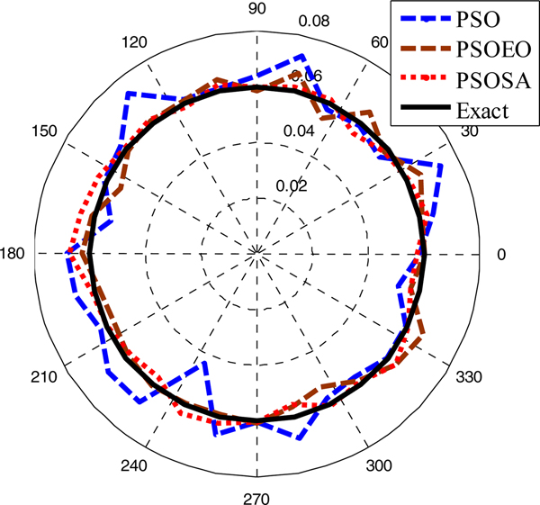
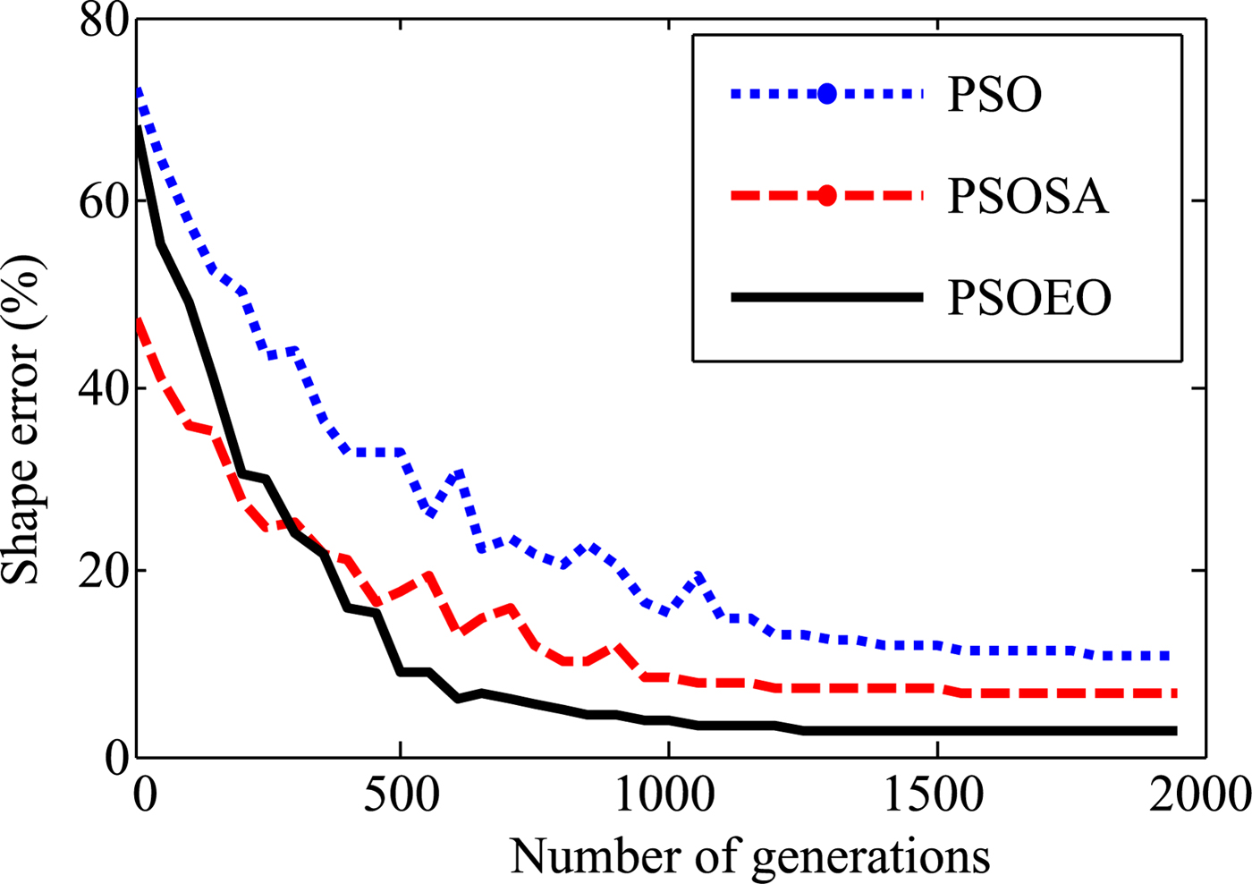
In the first example, a simple circular cylinder is examined, the shape function is chosen to be ρ(φ) = (0.06)m. The reconstructed shape function that corresponds to the best swarm particle is plotted in Fig. 4. The shape error is shown in Fig. 5. Here, the shape function discrepancy is defined as:
 $${\rm SE} = \left\{ {\displaystyle{1 \over Q}\mathop \sum \limits_{q = 1}^Q {\left[ {\displaystyle{{\rho^{cal}(\varphi_q)-\rho (\varphi_q)} \over {\rho (\varphi_q)}}} \right]}^2} \right\}^{{1 \over 2}}{\rm \;} $$
Fig. 4. Reconstructed results for the first example.

Fig. 5. Shape function error in each generation.
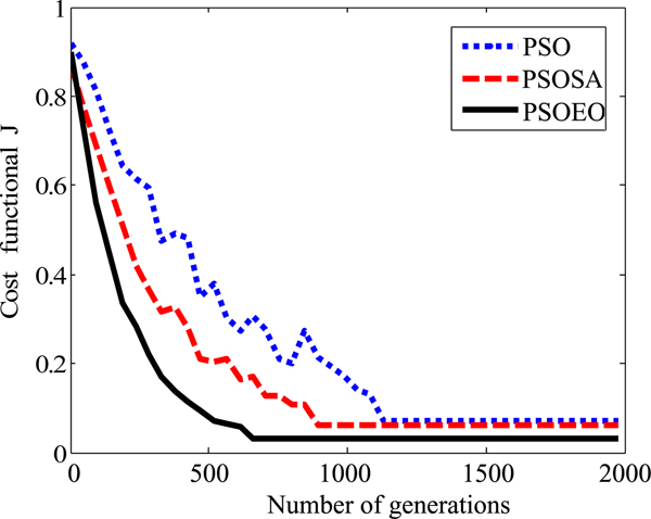
It is quite remarkable that the reconstructions are close to the exact shape of the object. However, it is clear that the best reconstructing is obtained by the hybrid algorithm PSOEO, indeed the shape error is of 10.3, 6.7, and 2.4% for PSO, PSOSA, and PSOEO, respectively. The convergence of the cost functional versus generations corresponding to the best particle in the swarm is shown in Fig. 6.

Fig. 6. The cost functional versus generation.
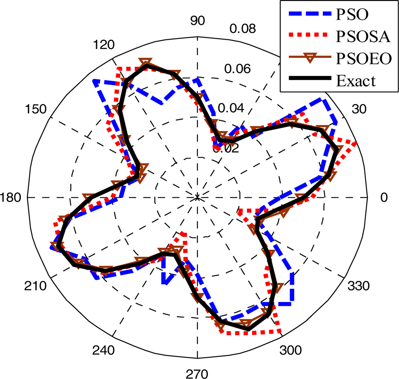
In the second example, we choose a shape function as ρ(φ) = (0.05 + 0.02 sin 4φ)m. In order to investigate the sensitivity of these algorithms against random noise, a Gaussian white noise is added to the real and imaginary parts of the simulated scattered fields. The signal-to-noise ratio (SNR) of different levels is used in our simulations. Figures 7 and 8 present the reconstructed shape using the three algorithms and the shape error, respectively. Figure 9 shows the reconstructed results where the experimental scattered field is contaminated by noise. It could be observed that good reconstructions of the perfect conducting cylinder have been obtained when the SNR is above 15 dB.

Fig. 7. Reconstructed results for the second example.
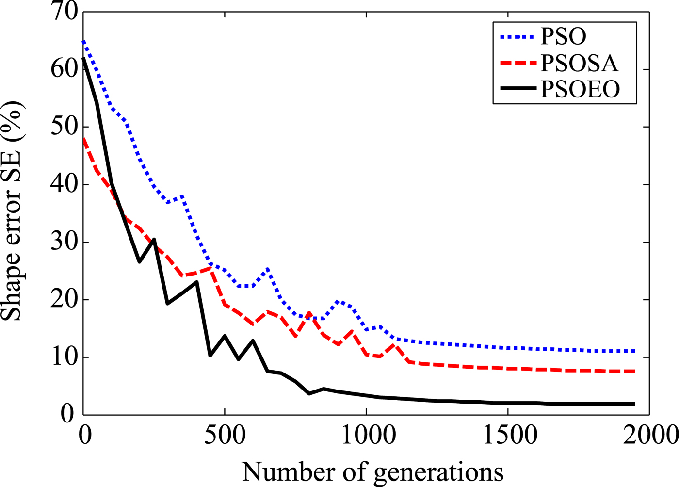
Fig. 8. Shape function error in each generation.
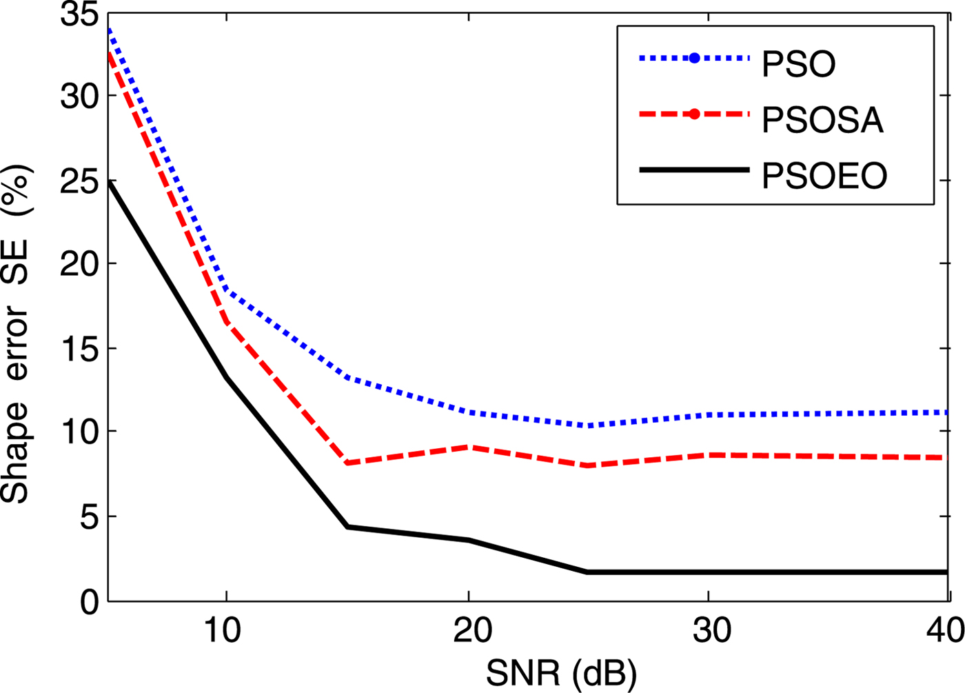
Fig. 9. The shape error as a function of SNR (dB).
Let us compare the three algorithms between them: it is clear that the two hybrid versions of PSO improved the reconstructing quality obtained by standard PSO. However, one observes that PSOEO is more effective than PSOSA algorithm especially against PSO, it presents less noise which is about 1.8% compared with 8.5 and 11.6% for PSOSA and PSO, respectively. Another advantage of PSOEO: it converges quickly, it put ~800 generations to reconstruct the object shape where more than 1200 iterations was necessary for the other algorithms.
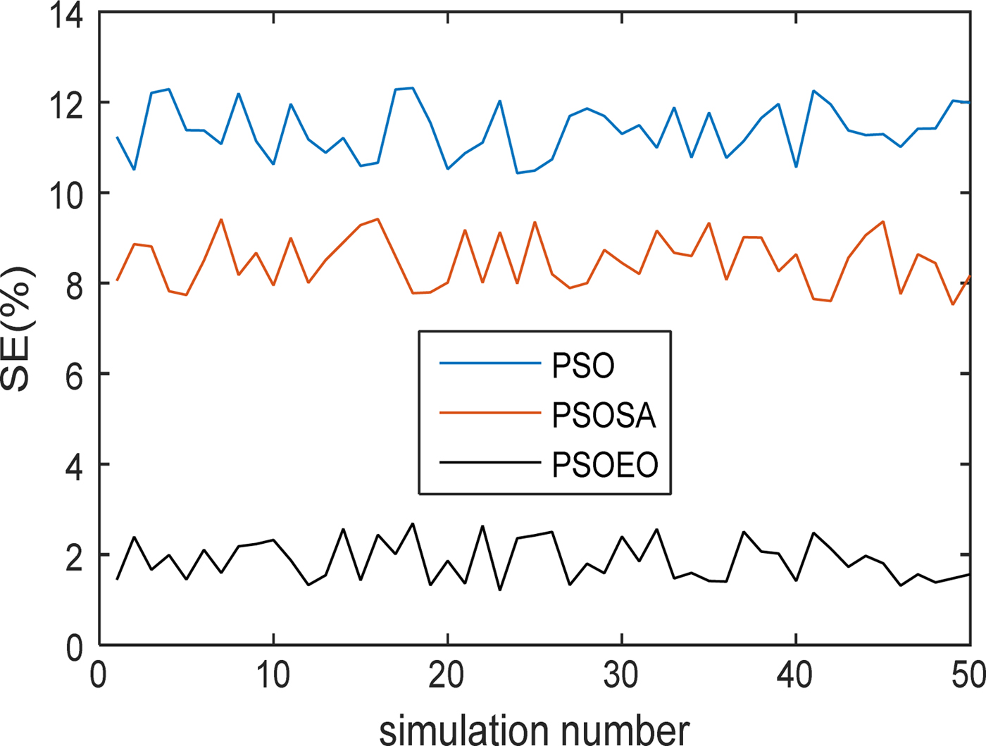
Another test of the used methods seems very interesting when they will be executed several times on this same second configuration whose purpose is to observe the variation of SE. Figure 10 illustrates the performance SE according to the execution of the three techniques PSO, PSOSA, and PSOEO.

Fig. 10. The shape error for 50 simulations.
It is clear that the convergences lead practically to the same values of SE obtained previously which are 11.6, 8.5, and 1.8% for PSO, PSOSA, and PSOEO, respectively.
Finally, what we can conclude is that these methods efficiently explore the solution space and provide good coverage to the actual form of the original configuration.
In [Reference Mhamdi, Grayaa and Aguili31], we developed a hybrid algorithm called mGA-CG combining a micro-GA and the method of the conjugate gradient. This technique allowed us to obtain good results for the reconstruction of the dielectric objects. It appears interesting to compare the performances of these different algorithms previously used with those of our own algorithm mGA-CG developed in [Reference Mhamdi, Grayaa and Aguili31]. To test the effectiveness of the algorithms as well as computing times, a third example is considered.
In the third example, the shape function is selected to be ρ(φ) = (0.03 + 0.02 sin φ + 0.01 sin 3φ + 0.02 cos φ)m. Note that the shape function is not symmetrical about either x axis or y axis. For this example, the reconstruction results are given in Table 1.
Table 1. Cost function, shape error, and computing time after convergence of algorithms for the third example

This example has further verified the reliability and fast convergence of PSOEO compared with PSO and PSOSA. For PSOEO and mGA-CG algorithms, almost they led to the same results and there is not a great difference between them. From the three examples already considered, we can observe clearly that the PSOEO algorithm is more effective than PSO and PSOSA. Thus the following comparison will be carried out only between PSOEO and mGA-CG.
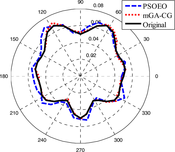
In the fourth example, the shape function is selected to be:
 $$\rho (\varphi ) = (0.05 + 0.02\,\sin\varphi \,\cos ^2\,3\varphi )m.$$
The reconstructed shape function that corresponds to the best swarm particle found by the two algorithms is plotted in Fig. 11.
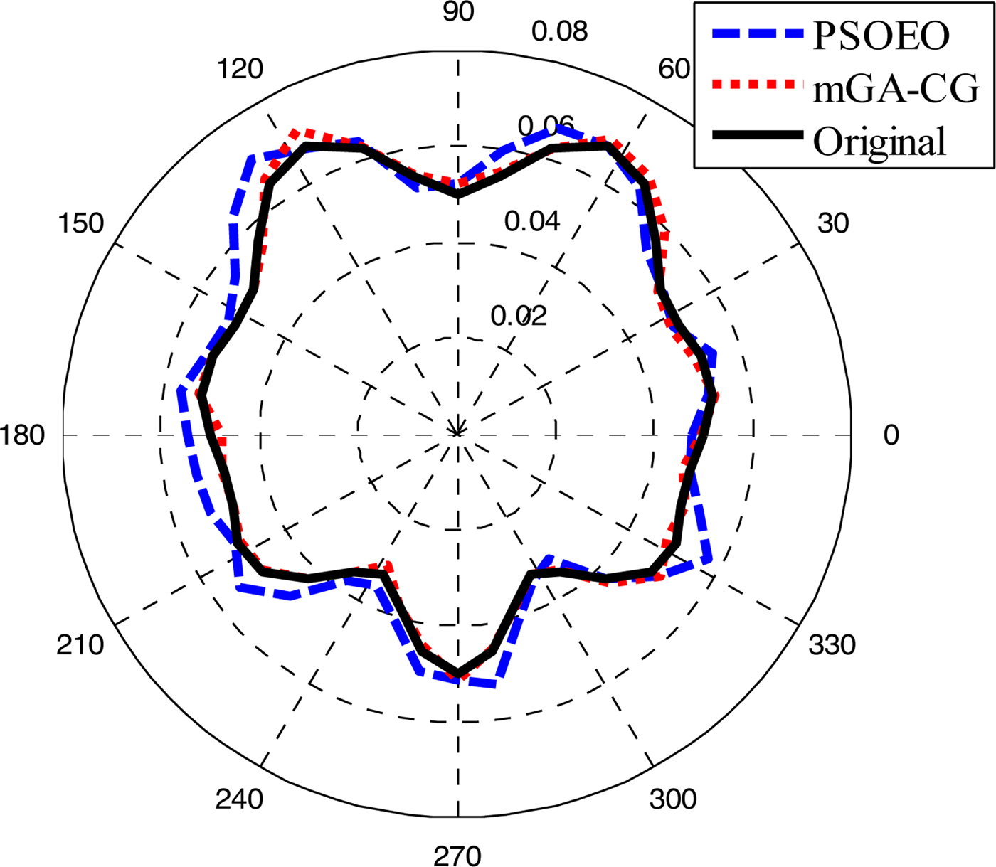
Fig. 11. Reconstructed results for the third example.
The fitness function, shape error, and computing time relative to each algorithm are given in Table 2.
Table 2. Cost function, shape error, and computing time for the fourth example

From Fig. 11, we observe that the mGA-CG algorithm reconstructs the original contour of the object contrary to the PSOEO algorithm which converges to a contour presenting some deformations. Thus, we notice that the hybrid technique mGA-CG showed more effectiveness than PSOEO, but one can say that these two algorithms are comparable.
Let's analyze more the results found and especially the two presented techniques advantages. For all considered examples, the performances are very close. However, it does not preclude recalling that the mGA-CG method uses the gradient which is a local technique which cannot always guarantee the convergence of the latter toward the real solution. On the other hand, our two methods PSOSA and PSOEO combine global techniques only and thus a better chance to reach the desired solution. In order to complete the study of the two methods, it is very interesting to see the effect of certain parameters namely the measurement data size given by m = M × I, the swarm size N, K max, and INV. The impact of these parameters is carried out on the fourth example studied previously.
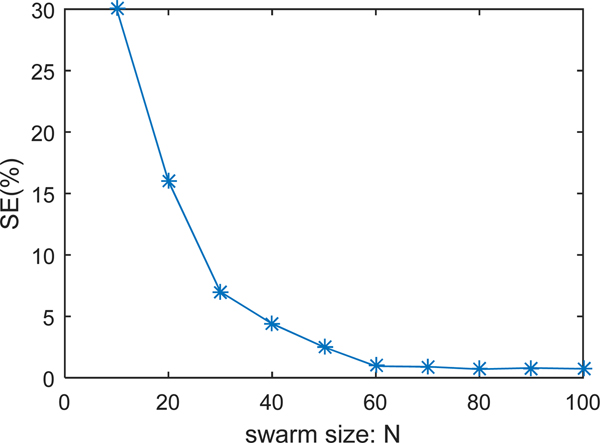
As an evaluation performance, we selected the shape error SE to detect the effect of these parameters. Figures 12 and 13 show the shape error evolution as a function of the number of measuring points m and the swarm size N, respectively. It is clear that more the m or N increase more a better reconstruction is obtained. We note also that from certain values of m and N, there will be no remarkable improvements.
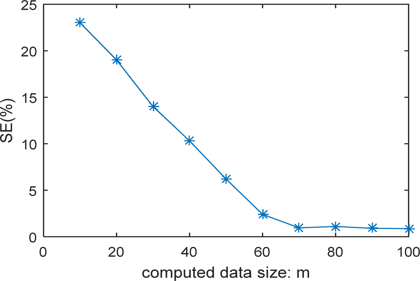
Fig. 12. Shape error versus measurement size.
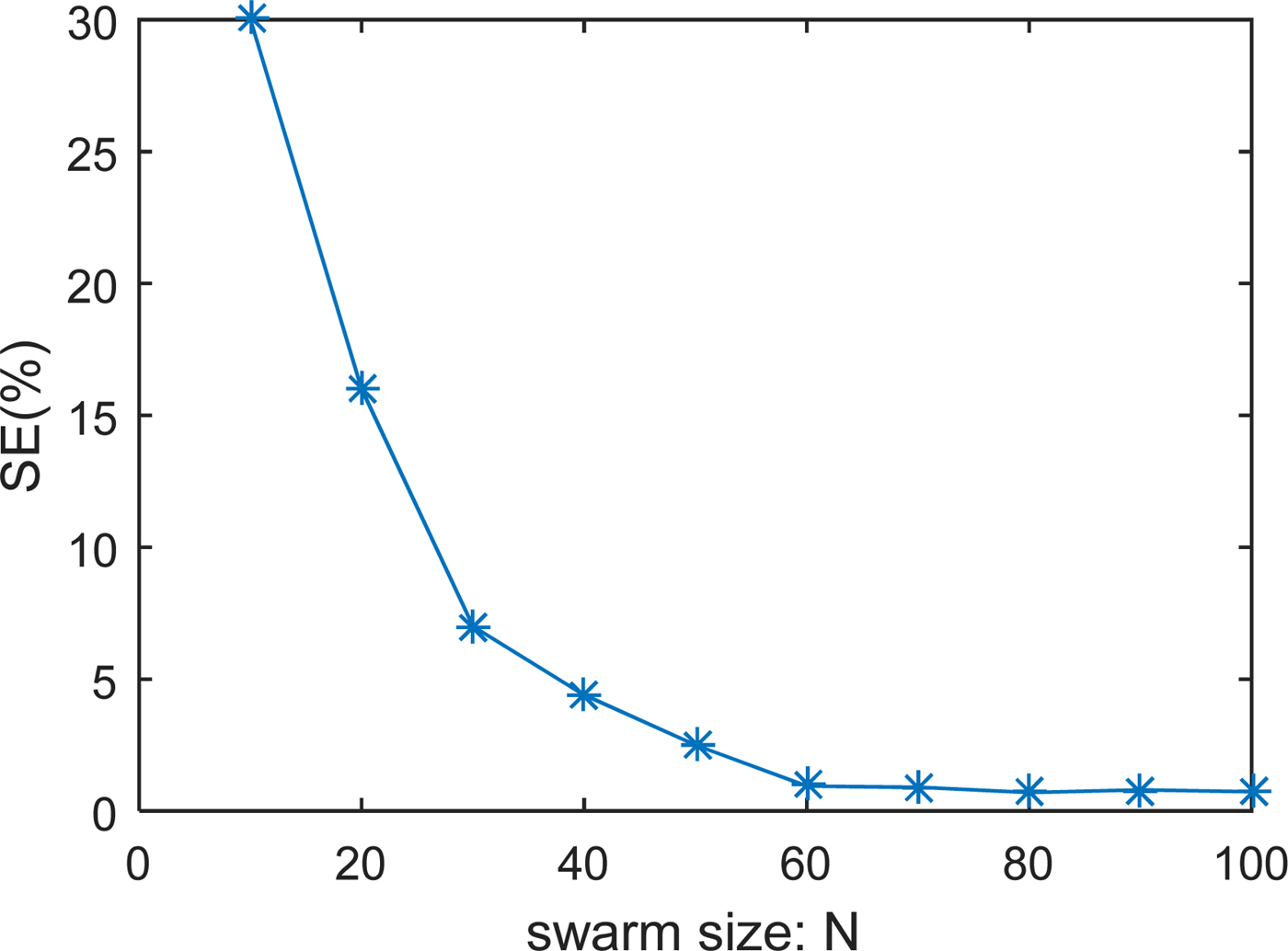
Fig. 13. Shape error versus swarm size.
In order to properly evaluate the robustness and the favor that these two hybrid algorithms can provide, a comparison with SA and EO is made. The two performances computational cost SE and the calculation time will be carried out during the reconstruction of the fourth case.
Table 3 shows the results of simulations obtained for the four algorithms, PSOSA, PSOEO, SA and EO. It is clear that PSOEO converges better compared with others and more robust than PSOEO for both performances. If we compare the hybrid methods with those with single agent (SA and EO), it is shown that SA and EO are faster while hybridization has improved the quality of reconstruction. So there is a tradeoff between computing time and computational cost.
Table 3. Shape error and computing time after convergence of algorithms for the fourth example

Another simulation of K max and INV effects is performed. Table 4 illustrates the simulation results for shape error by applying the two PSOSA and PSOEO techniques while varying K max and INV respectively. From these results, we can notice that for low values of K max and INV or from a certain threshold the SE becomes large. A better choice of K max for PSOSA and INV for PSOEO should be around 40 and 50, respectively.
Table 4. Shape error for different values of K max and INV for the fourth example

Conclusion
Two hybrid optimization methods called PSOSA and PSOEO for reconstructing the shape of perfectly conducting cylinders by TM waves have been employed. The forward problem is solved by using the MoM and the contour of the cylinder is approximated by Fourier series expansion. The computational results indicate that the algorithms appear to produce very good reconstructions of the object shape from the scattered fields even in the presence of the measurement noises. Compared with standard PSO and PSOSA, it has been shown that the PSOEO approach has better performances in terms of accuracy, convergence rate, stability, and robustness. The PSOEO algorithm is also compared with our own technique named mGA-CG and a superiority of this last method concerning the precision and the convergence speed is recorded. However, these illustrated algorithms are random and to support one compared with another requires a sufficient number of tests and evaluations. Finally, these two techniques can be regarded as a powerful optimization tool for the electromagnetic problems especially in microwave imaging.
Acknowledgments
We would like to express our sincere thanks and appreciation to SYSCOM Laboratory and ENIT for their help and support in developing this paper.
 Bouzid Mhamdi was born in Kasserine, Tunisia, on June 7, 1977. He received his electrical engineering degree (2002) and M.Sc. (2004), and Ph.D. (2011) in telecommunication from the National Engineers School of Tunis, Tunisia. At present, he works at the University of Kairouan, ISSAT Kasserine as an Associate Professor in Communications Engineering Department. His current research interests include forward and inverse electromagnetic problems for microwave imaging and MIMO systems.