Passive location system based on troposcatter

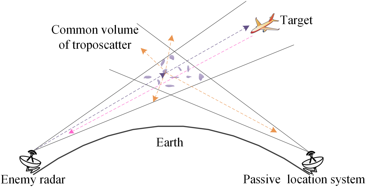
Figure 1 depicts passive location system based on troposcatter, which can effectively make a b-LoS detection and counter the anti-radiation missile. To obtain the location of enemy radar, it has at least three stations [Reference Zhuang and Wang12]. Distributed system has an inherent superiority at realizing CSD, which can effectively resist the undesirable shadow and multipath fading.

Fig. 1. Passive location system based on troposcatter.

Only system makes a faultless decision, the next works will be carried out. In CSD, each node independently detects the signal and FC makes a global decision based on data fusion or decision fusion. The former consumes more wireless resources. On the other hand, performance of the latter could be improved remarkably by increasing the number of nodes [Reference de Paula and Panazio13].

As shown in Fig. 2, each terminal node of passive location system can be regarded as a FC. Local decision can be delivered by the reporting channel. According to decision fusion, u _i stands for the decision of node i, here u _i = 1 for the signal is present and u _i = 0 for the decision of absent signal. AND-rule and OR-rule can be adopted for decision fusion, the latter has a good performance and wide application [Reference Yue, Zheng, Meng, Cui and Xie14]. According to OR-rule, FC can make global decision under an ideal condition as

(1)$$\left\{ {\matrix{ {Q_{FA} = 1 - \prod\limits_{i = 1}^L {(1 - P_{FA})},} \cr {Q_D = 1 - \prod\limits_{i = 1}^L {(1 - P_D)},} \cr}} \right.$$

where Q _FA stands for the global probability of false alarm, Q _D the global probability of detection, L the number of terminal nodes, P _FA the terminal probability of false alarm, P _D the terminal probability of detection. Considering bit error rate (BER) of the reporting channel, we can obtain Q _FA and Q _D as

(2)$$\left\{ {\matrix{ {Q_{FA} = 1 - \prod\limits_{i = 1}^L {[(1 - P_{FA})(1 - P_e) + P_{FA}P_e} ],} \cr {Q_D = 1 - \prod\limits_{i = 1}^L {[(1 - P_D)(1 - P_e) + P_DP_e]},} \cr}} \right.$$

where P _e refers to the BER. Detection problem can be transformed into a binary hypothesis test, thus

(3)$$\left\{ {\matrix{ {H_0:r\lsqb n \rsqb = w\lsqb n \rsqb } \hfill \cr {H_1:r\lsqb n \rsqb = s\lsqb n \rsqb + w\lsqb n \rsqb } \hfill \cr} \matrix{ {} & {n = 0,1, \cdots, N - 1,} \cr {} & {n = 0,1, \cdots, N - 1,} \cr}} \right.$$

where H ₀ refers to the absence of a signal, H ₁ the presence of a signal, s[n] the unknown deterministic signal, w[n] the additive white Gauss noise (AWGN) with zero mean and σ ² variance. According to ED [Reference Chatziantoniou, Allen, Velisavljevic, Karadimas and Coon15], observed energy of signal can be expressed as

(4)$$Y = \displaystyle{1 \over M}\sum\limits_{n = 1}^M {{\vert {r(n)} \vert } ^{^2}}, $$

where Y denotes the observed energy, M the number of samples taken under an observation period. If Y > τ, s[n] is present, otherwise the signal is absent. Here, τ stands for the predefined threshold. P _FA and P _D can be given as

(5)$$\left\{ {\matrix{ {P_{FA} = \Pr (Y \gt \tau \vert {H_0} ) = Q\left( {\displaystyle{{\tau - \sigma^2} \over {\sigma^2\sqrt {{2 / M}}}}} \right),} \cr {P_D = \Pr (Y \gt \tau \vert {H_1} ) = Q\left( {\displaystyle{{{\tau / {\sigma^2}} - (1 + \gamma )} \over {\sqrt {{2 / M}} (1 + \gamma )}}} \right),} \cr}} \right.$$

where γ denotes the SNR, Q(.) the Gaussian complement integral function, which can be given by

(6)$$Q(x) = \displaystyle{1 \over {\sqrt {2\pi}}} \int_x^{ + \infty} {e^{ - u^2/2}} du.$$

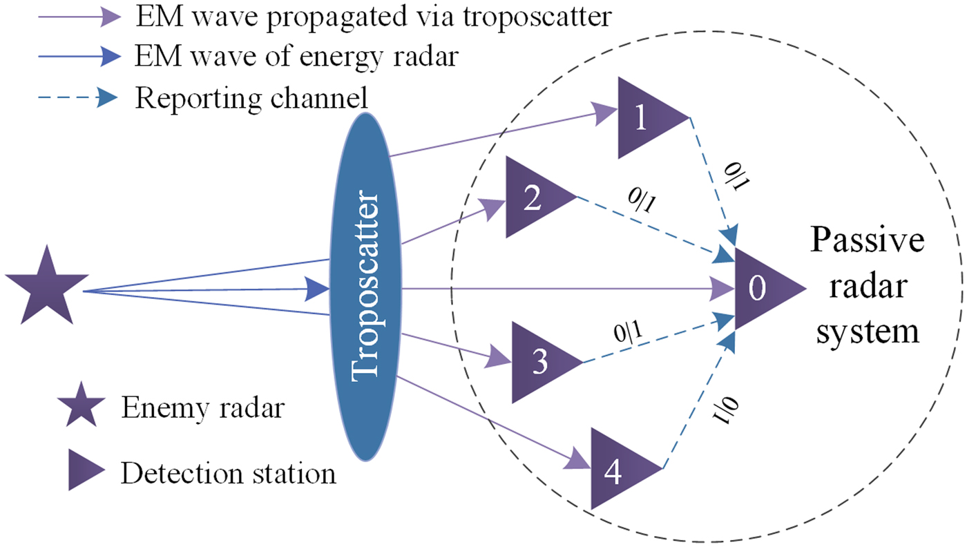
Fig. 2. Layout of CSD.

Troposcatter can be approximated as a Rayleigh fading channel [Reference Li, Chen and Liu16], we can acquire the probability distribution function of average SNR as

(7)$$f\,(\gamma ) = \lpar {{1 / {\bar \gamma}}} \rpar e^{ - ({\gamma / {\bar \gamma}} )},$$

where ${ \bar {\gamma} }$ refers to the average SNR. Therefore, P _D can be given by

(8)$$P_D = \int_0^\infty {Q\left( {\displaystyle{{{\tau / {\sigma^2}} - (1 + \gamma )} \over {\sqrt {{2 / M}} (1 + \gamma )}}} \right)f\lpar \gamma \rpar } d\gamma. $$

An unstable environment can lead to varying noises. The uncertainty parameter of noises is uniformly distributed and can be expressed as

(9)$$\rho = \displaystyle{{\sigma _u^2} \over {\sigma ^2}} \in [10^{ - A{\rm /10}},\,\,10^{A{\rm /10}}],{\kern 1pt} {\kern 1pt} {\kern 1pt} A \ge 0.$$

Figure 3 shows the principle of double-threshold ED [Reference Verma and Singh8, Reference Ahuja and Kaur17], which is accepted as a viable solution to copying with the defect caused by varying noises. λ ₁ and λ ₂ denote two thresholds, which can be expressed as

(10)$$\left\{ {\matrix{ {\lambda_1 = \left( {\sqrt {\displaystyle{2 \over M}Q^{ - 1}(P_f) + 1}} \right)\displaystyle{1 \over \rho} \sigma_{}^2} \cr {\lambda_2 = \left( {\sqrt {\displaystyle{2 \over M}Q^{ - 1}(P_f) + 1}} \right)\rho \sigma_{}^2} \cr}} \right..$$

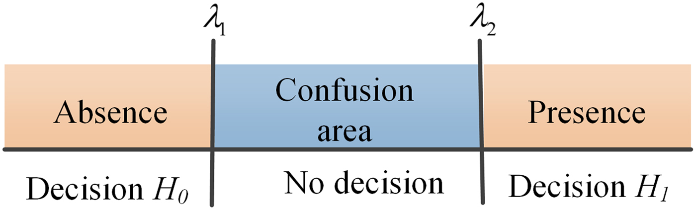
Fig. 3. Principle of double-threshold ED.

As equation (10), ρ and σ ² need to be precisely estimated. A confusion area exists between λ ₁ and λ ₂.

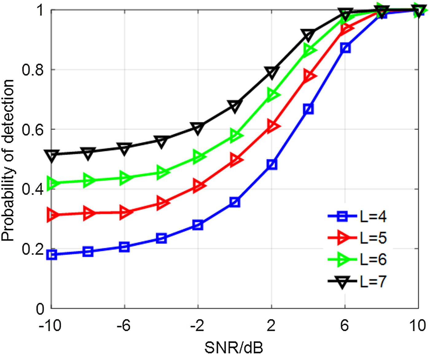
Figure 4 shows the P _D of CSD with the parameter P _FA = 0.01, A = 0.5, σ ² = 1, P _e = 10⁻⁴. It indicates that SNR has a great effect on signal detection. Meanwhile, large number of terminal nodes can lead to a better performance.

Fig. 4. P _D of CSD.

The main drawback of double-threshold ED is the confusion area and dependence on knowledge of background noises. Low SNR can contribute a poor performance to double-threshold ED. As known, troposcatter has a relatively high propagation loss and the received signal suffers from low SNR. Therefore, signal detection with good performance is in urgent need.

Blind signal detection

Filtering model

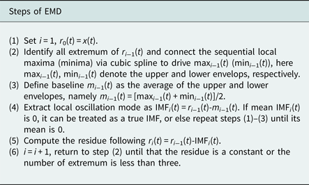
Empirical mode decomposition (EMD) based on Hilbert–Huang transform can decompose any complex signal into several sequences, which can be designated as intrinsic mode functions (IMFs). Every IMF represents a simple oscillatory mode [Reference Li, Wang, Zhang and Tang18]. Steps are as follows.

The final consequences of EMD can be given by

(11)$$x(t) = \sum\limits_{i = 1}^n {h_i(t)} + r_n(t),$$

where x(t) denotes the original signal, r _n(t) the remainder term, h _i(t) the ith IMF. Each h _i(t) has a single frequency. The first m IMFs with high frequency are usually treated as background noises. The clean signal f(t) and noises s(t) can be reconstructed as

(12)$$\left\{ {\matrix{ {\,f\,(t) = \sum\limits_{i = m + 1}^n {h_i(t)} + r_n(t),} \cr {s(t) = \sum\limits_{i = 1}^m {h_i(t),\;\;\;\;\;\;\;\;\;\;}} \cr}} \right.$$

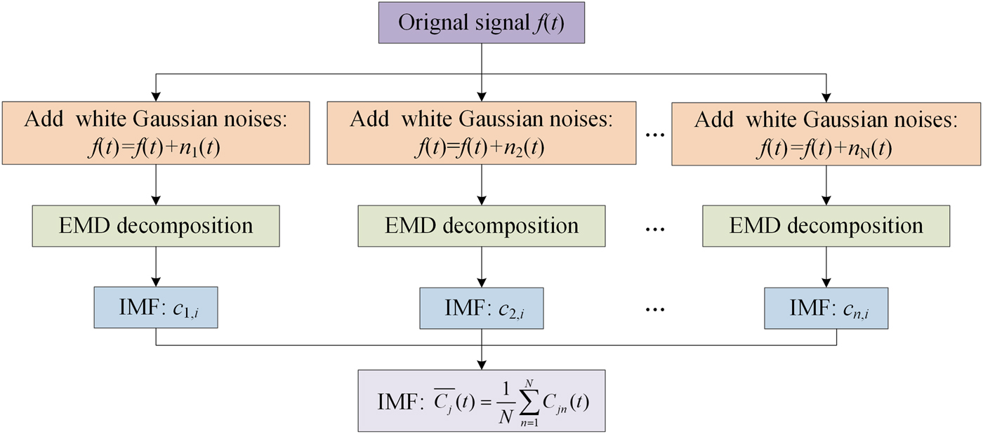
The primary weakness of EMD is mode mixing, which can be defined as a single IMF including oscillations of dramatically disparate scales, or a component of similar scale residing in different IMFs. When a signal is affected by interference, this problem is more likely to exist. Ensemble EMD (EEMD) can effectively copy with mode mixing [Reference Liu, Cui and Li19]. According to EEMD, white noises are repeatedly added to the original data. Aim of above step is to homogenize signal scale in time-frequency space. As usual, variance of added white noise is 0.2$\sigma _s^2 $, here $\sigma _s^2 $ is the variance of original data.

Figure 5 shows the process of EEMD, here, $\sqrt N = 0.2\sigma _s^2 /e$. To regulate the precision and running time, value of e is usually assigned as 0.01. However, EEMD brings a new problem that the signal will be inevitably polluted by added white noises. Complementary EEMD (CEEMD) can reduce the reconstruction errors caused by the added white noises. According to CEEMD [Reference Xu, Luo, Li and Song20], white noises are added in pairs to the signal. The chief innovation of CEEMD can be expressed as

(13)$$\left\{ {\matrix{ {r_{ij}^ + (t) = f\,(t) + n_i(t),} \cr {r_{ij}^ - (t) = f\,(t) - n_i(t).} \cr}} \right.$$

Fig. 5. Process of EEMD.

Above noise-added data are decomposed via EMD. $c_{ij}^ + (t)$ ($c_{ij}^ - (t)$) represents the jth IMF derived from the ith noise-added data. The final IMF can be obtained as

(14)$$\hbox{IM}\hbox{F}_j(t) = \displaystyle{1 \over N}\sum\limits_{n = 1}^N {[c_{i,j}^ + (t) + c_{i,j}^ - (t)]}. $$

As stated above, CEEMD can guarantee relatively actual IMFs. Then, the main problem is to determine parameter m in equation (12). To indicate uncertainty of determining m, we employ Heavysine signal added with different white noises as a reference. After decomposing signal on the basis of CEEMD, we successively reconstruct the signal and background noises according to equation (12). SNR is employed to evaluate the consequence, which is defined as

(15)$$SNR = 10\lg \left[ {\displaystyle{{\sum\nolimits_{k = 1}^M {s_k^2}} \over {\sum\nolimits_{k = 1}^M {{(s_k - g_k)}^2}}}} \right],$$

where s _k denotes the original Heavysine signal, g _k the reconstructed signal, M the sampling points. SNR with higher amplitude indicates that the reconstructed signal is more coincident with original signal. Namely, eliminated noises is more authentic.

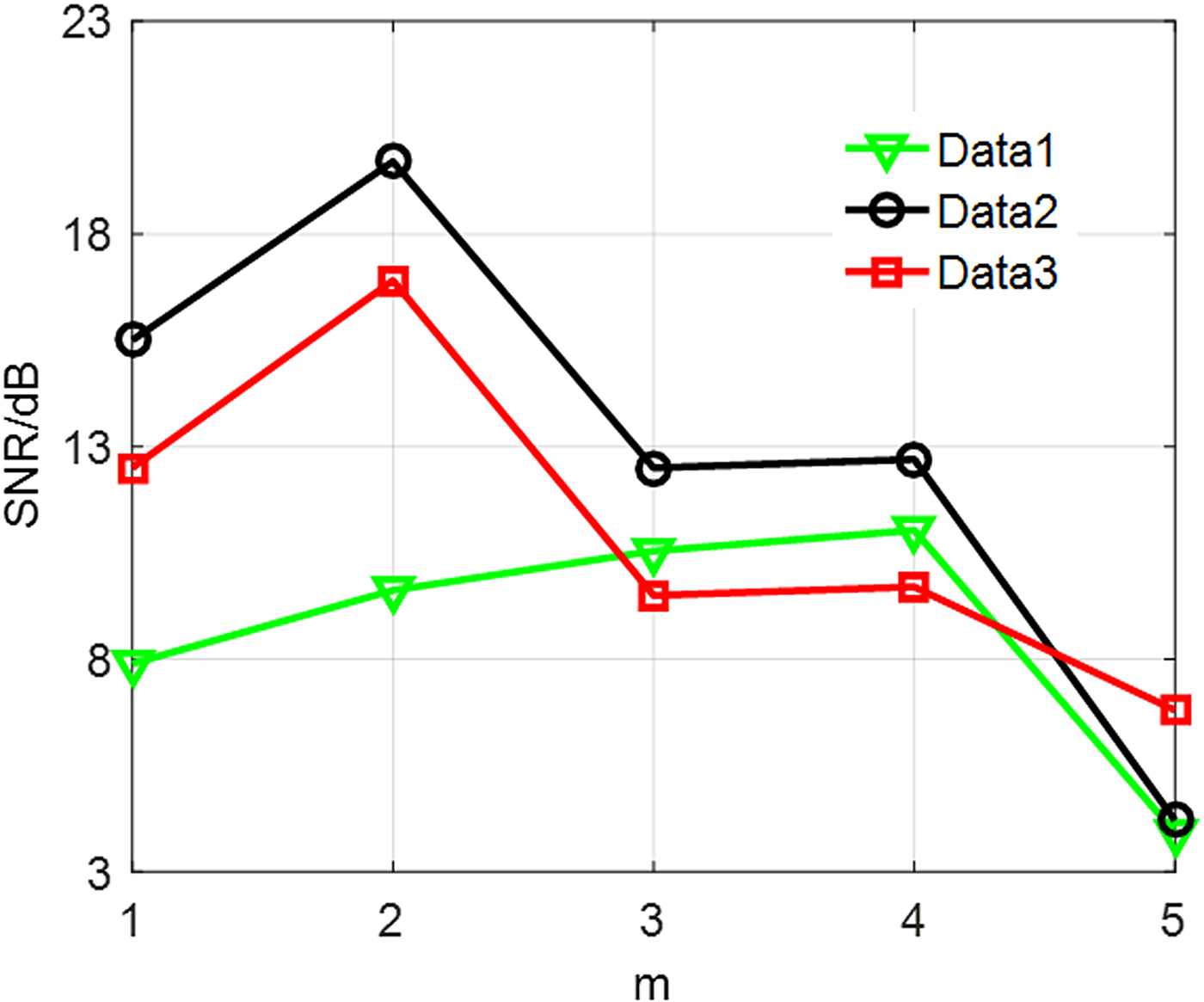
Figure 6 displays SNR corresponding to different m. The respective characteristics of signals lead to different optimal m. Therefore, determining m is relatively difficult and needs abundant experiment. To accurately recognize IMFs, principal component analysis (PCA) is employed [Reference Sharifi and Langari21]. However, complex matrix operation existing in PCA may lead to a long running time. Entropy theory is accepted as an effective way to explicitly depict a signal, which can be expressed as [Reference Lim and Yuen22]

(16)$$H(x) = - \sum\limits_{i = 1}^L {P(x = a_i)\log} [P(x = a_i)],$$

where P(x = a _i) stands for the probability of x = a _i. Entropy with a bigger value indicates that the signal is more unsteady and contains much more noises. The entropy of adjacent IMF is employed as a standard. Approach to determine m can be presented as follows.

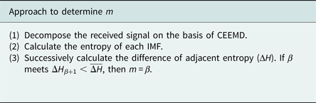
Fig. 6. SNR of proposed signals.

Here

(17)$$\overline {\Delta H} = \displaystyle{1 \over {n - 1}}\sum\limits_{i = 1}^{n - 1} {\Delta H_i}, \;\;\Delta H_i = H_i - H_{i + 1}.$$

Signal detection based on ED and filtering model

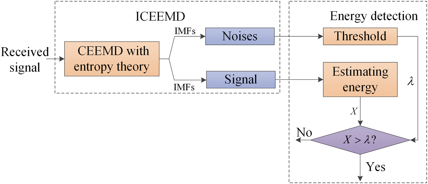
Figure 7 shows the process of blind signal detection proposed in this paper. Firstly, CEEMD adaptively decomposes the signal received by passive system. Then, entropy theory described by equations (16) and (17) is used to precisely recognize consequences. IMFs treated as noises can be employed to calculate threshold of ED. Meanwhile, residual IMFs are used to estimate the observed energy on the basis of equation (4). In this way, SNR can be obviously enhanced. Because of CEEMD and entropy theory, the signal detection proposed in this paper can run without human intervention, threshold can be constantly updated during the signal detection running. Because complicated matrix operations do not exist, its complexity can be approved.

Fig. 7. Process of blind signal detection.

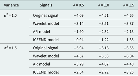
To indicate the superiority of improved CEEMD (ICEEMD) model, a monopulse radar is treated as our target. Pulse wave added with AWGN is employed as received signal, amplitude and duty ratio of pulse wave is 2 and 5%, respectively. ICEEMD, wavelet, and AR models are employed to process the received signal. SNR described in equation (15) is also treated as a standard. Parameters of wavelet model have varied styles. After repeated simulations, model with db5 function, scale 5, and soft threshold function has the best performance among different wavelet models. Table 1 shows SNR of original signals and signals processed by different models. From Table 1, SNR is obviously enhanced by the filtering models to a certain extent. ICEEMD can most precisely reconstruct the signal. As well, AR model performs better than wavelet model.

Table 1. SNR of original and processed signals.

Example analysis

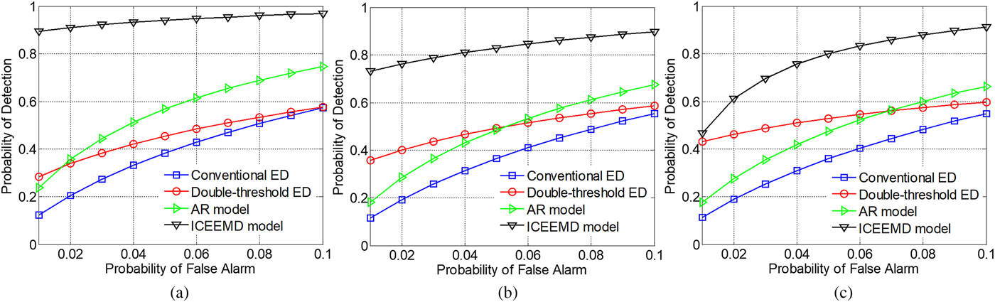
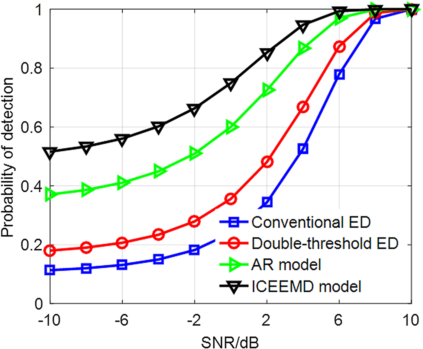
In this section, above pulse wave with AWGN is also employed to imitate received signal. Figure 8 displays receiver operating characteristic of different ED with parameters: A = 0.5, σ ² = 1, L = 4, P _e = 10⁻⁴. Abscissa denotes the probability of false alarm; ordinate denotes the theoretical probability of detection. For conventional ED, threshold is estimated according to the background noises extracted by ICEEMD; original received signal is employed to estimate the energy level. For double-threshold ED, A and σ ² are available. ICEEMD model denotes the blind signal detection proposed in this paper. Because AR model performs better than wavelet model, we employ it as a reference. Similar to ICEEMD model, background noises and observed energy are estimated by the AR model. Figure 9 shows theoretical P _D changing with SNR with the same parameters and P _FA = 0.01. Abscissa denotes the SNR of received signal.

Fig. 8. ROC of energy detection improved by different models. (a) A = 0.5; (b) A = 1.0; (c) A = 1.5.

Fig. 9. SNR of signal processed by different models.

As shown in Fig. 8, ICEEMD model can better improve ED than AR model. Although double-threshold ED can somewhat improve the performance of signal detection, knowledge of background noises must be available.

Figure 9 also indicates the superiority of the blind signal detection algorithm proposed in this paper. Because ICEEMD and AR models can enhance the SNR, these two models have better performance with the low SNR than conventional models. During above simulations, the blind signal detection can run without priori knowledge and user intervention.