


Introduction
The recent works [Reference Jany, Siligaris, Ferrari and Vincent1–Reference Siligaris, Iskandar and Guerra7] have demonstrated a novel frequency-synthesis methodology, based on the high-order sub-harmonic injection-locking of a high-frequency oscillator, at a frequency fo, by an independent source at a much lower frequency fin. In [Reference Jany, Siligaris, Ferrari and Vincent1–Reference Jany, Siligaris, Ferrari and Vincent3], the high ratio N between the two frequencies (in the order of N = 30) is achieved by shaping the input sinusoidal signal into a square signal that periodically switches on and off a high-frequency oscillator. This is used to injection lock a second oscillator that selects the harmonic closest to its own free-running frequency. The procedure has two advantages. On the one hand, as demonstrated in [Reference Jany4], the phase-noise spectral density of the higher-frequency oscillator can be lower than the one resulting from lower sub-harmonic ratios (due to the higher phase-noise of the required input source). On the other hand, the availability of a high number of equally spaced spectral lines enables a programmable carrier generation. Actually, the second injection-locked oscillator in [Reference Jany, Siligaris, Ferrari and Vincent1–Reference Jany, Siligaris, Ferrari and Vincent3] enables the selection of one or another spectral line (with the frequency spacing fo/N) depending on its tuning voltage. The whole system has the advantage of low phase noise in comparison with standard phase-locking methodologies [Reference Jany, Siligaris, Gonzalez-Jimenez, Vincent and Ferrari2, Reference Jany4].
Successful experimental demonstrations of this promising frequency-synthesis method, as well as several extensions of the new procedure, have been presented in [Reference Jany, Siligaris, Ferrari and Vincent1–Reference Siligaris, Iskandar and Guerra7]. However, the realistic simulation of the high-order sub-harmonic injection-locked oscillator, required for an accurate prediction of its behavior, is involved. In general, full time-domain simulations, which often fail in the presence of distributed elements, are only possible with simplified models of the circuit components, as done in [Reference Jany, Siligaris, Ferrari and Vincent1–Reference Jany, Siligaris, Ferrari and Vincent3], where models of the Van der Pol type are used to describe the transistor devices. In [Reference Jany, Siligaris, Ferrari and Vincent1–Reference Jany, Siligaris, Ferrari and Vincent3], an approximate analytical formulation in time-domain is proposed, in which the synchronized states are detected through a comparison of the oscillation amplitude and phase values at the beginning and end of each period of the switching signal. On the other hand, though harmonic balance (HB) [Reference Kundert8–Reference Quere, Ngoya, Camiade, Suarez, Hessane and Obregon12] can deal at present with a high number of harmonic terms, in injection-locked oscillators it converges by default to the non-oscillatory solution that generally coexists with the oscillatory one. In the non-oscillatory solution, the circuit just responds to the input forcing in a non-autonomous manner [Reference Ramirez, de Cos and Suarez13–Reference Hernández, Pontón, Sancho and Suárez15]. To consider the self-oscillation in commercial HB, one should impose the oscillation condition using an auxiliary generator (AG) [Reference Ramirez, de Cos and Suarez13–Reference Hernández, Pontón, Sancho and Suárez15]. The AG amplitude and its phase-shift with respect to the input source are optimized to obtain a zero value of the AG total admittance function. In the case of a sub-harmonic injection locking of a high order N, the convergence of this optimization procedure is demanding [Reference Hernández, Pontón, Sancho and Suárez15] due to the need of a high number NH of harmonic terms, involving multiples of the high order N. For instance, the consideration of three harmonic components of the oscillation frequency fo, requires NH = 3N = 90.
This work is an extension of [Reference Hernández, Pontón, Sancho and Suárez15], presenting an envelope-domain analysis [Reference Ngoya and Larcheveque16–Reference Carvalho, Pedro, Jang and Steer19] of the sub-harmonic injection-locked oscillator is presented, using a Fourier-series description of the circuit variables, with time-varying harmonic terms $\bar{X}_k\lpar t\rpar$ , where k is the frequency index. This will require a proper initialization of the oscillation frequency to avoid the system convergence to a non-oscillatory steady-state solution [Reference Cos, Suarez and Sancho20]. As will be shown, it is possible to choose different fundamental frequencies, expressed as fo/P where P is an integer. For P > 1, the spectral lines of the sub-harmonic regime are distributed among the harmonic components kfo/P of the Fourier representation of the circuit variables. Then, even in injection-locked conditions, the harmonic terms $\bar{X}_k\lpar t\rpar$
 will exhibit time variations due to the spectral lines contained in the bandwidth about each harmonic frequency kfo/P, so a criterion is needed for efficient detection of the synchronization bands. In order to derive this criterion, a semi-analytical formulation in the envelope-domain, based on an admittance-type model of the oscillator circuit, will be initially considered. An analytical expression will be derived, demonstrating that the injection-locked states can be efficiently detected through the averaging oscillator phase. In addition, the closed solution curves, characteristic of the injection-locked operation [Reference Suárez10–Reference Ramirez, de Cos and Suarez13], will be obtained through an averaging of the envelope amplitude.
In the solution of the sub-harmonic injection-locked oscillator, there will be a high number of spectral lines at multiples of the low injection-locking frequency fin. This can be achieved through pulse forming plus oscillator switching, as in [Reference Jany, Siligaris, Ferrari and Vincent1–Reference Jany, Siligaris, Ferrari and Vincent3], or using of a multi-harmonic input source, as in this work. As proposed in [Reference Jany, Siligaris, Ferrari and Vincent1–Reference Jany, Siligaris, Ferrari and Vincent3], the selection of a particular spectral line can be carried out connecting the oscillator output to a second oscillator circuit (in the same frequency order) with frequency tuning capabilities. The injection-locking (at the fundamental frequency) of this second oscillator enables the selection of one or another spectral line by varying its tuning voltage. Here, this frequency selection by means of injection locking will be analytically investigated considering an oscillator injected with multiple closely spaced input tones.
The phase-noise analysis of the high-order sub-harmonic injection-locked oscillator will be addressed here for the first time to our knowledge. This analysis is demanding, since, as stated, the HB analysis will fail to converge in most cases due to the need to fulfil the oscillation condition under a high number of harmonic terms. On the other hand, a Monte-Carlo phase-noise analysis in the envelope domain is virtually impossible, due to the presence of two widely separated time scales, one associated with the noise perturbation and the other one accounting for the bandwidth about each harmonic term. Even for P = N, the integration time step required to obtain convergence to the oscillatory solution will generally be much smaller than the total simulation time needed to account for the effect of the noise sources. Here the phase noise will be studied in two different manners. First, the phase-noise spectrum will be analytically derived from a perturbation analysis at the oscillation frequency, relying on an admittance-type model [Reference Ramirez, Ponton, Sancho and Suarez21] of the oscillator circuit in its injection-locked steady state. This formulation will allow an understanding of the frequency response of the sub-harmonic injection-locked oscillator with respect to the input-source noise and its own noise sources. Then, a procedure to identify the key parameters defining the spectrum shape from circuit-level envelope-transient simulations will be proposed. The whole methodology will be applied to a sub-harmonic injection-locked oscillator at the order N = 30, which has been manufactured and measured.
The paper is organized as follows. In the section “Oscillator injected by multiple input tones”, the response of an oscillator driven by multiple periodic tones with a small frequency spacing will be presented. In the section “Sub-harmonic injection-locked operation”, the envelope-domain analysis of a sub-harmonic injection-locked oscillator under a high order N will be described. The section “Phase noise” presents the derivation of the phase-noise spectrum in the frequency domain, as well as a procedure to identify the parameters that define this spectrum through envelope-transient simulations.
Oscillator injected by multiple input tones
In this section, the case of an oscillator injected with multiple input tones about the oscillation frequency will be studied [Reference Hernández, Pontón, Sancho and Suárez15], which is conceptually simpler than the one of sub-harmonic injection-locked oscillators under a high order N, considered in the section “Sub-harmonic injection-locked operation”. This will allow an understanding of the oscillator behavior when driven by multiple tones and an evaluation of its frequency-selection capabilities. A criterion will be derived to determine the locking ranges about each input tone when a parameter is varied, which will be extended in the section “Sub-harmonic injection-locked operation” to the sub-harmonic injection-locked oscillator.
Analytical formulation
A set of input tones will be introduced into the oscillator circuit, at the frequencies ω 1, ω 2,…, ωK, assumed to be closely spaced about the original free-running oscillation frequency ωo. When varying a suitably chosen tuning parameter η, the oscillator should be able to lock to each of the different input frequencies ωk. To get analytical insight, the oscillator will be described at its fundamental frequency, in terms of its current-to-voltage ratio Y(V,ω,η) at a particular observation node [Reference Suarez, Ramirez and Sancho22–Reference Fernández, Ramírez, Suárez and Sancho26], where V and ω are the excitation amplitude and frequency. This admittance function will be the current-to-voltage ration of an AG connected at the observation node in the HB simulation of the oscillator circuit. In the absence of the input signals, at its free-running solution, the oscillator fulfils the following two-tier equation system [Reference Suárez and Quéré11]:

where $\bar{H}$ represents the HB system that constitutes the inner tier and Vo and ωo, are the free-running amplitude and frequency at ηo. Note that the phase origin has been arbitrarily taken at the observation node Vej 0 and the vector $\bar{X}^{\prime}$
 contains all the state variables except Vej 0. The above system can be solved through optimization of V and ω in order to fulfil the goal Y = 0.
Now, the effect of the input source will be considered. Injection-locking to the particular input tone ωq, belonging to the set of input tones ω 1, ω 2,…,ωK, will be assumed. The oscillator will be formulated in the envelope domain at the carrier frequency ωq. Thus, the node voltage will be expressed as $\lpar {V_o + {\rm \Delta }V\lpar t\rpar } \rpar e^{j\phi \lpar t\rpar }e^{j\omega _qt}$ , where ΔV(t) is the time-varying increment of the voltage amplitude with respect to the free-running value Vo and ϕ(t) is the time-varying phase, in the presence of the input sources. Applying Kirchoff's laws at the observation node one obtains the following system:

where Δω q = ω q − ω oand s is a complex frequency increment and Ik is the equivalent complex current associated with each input signal. Note that Δω k,q is the offset frequency of each input tone k ≠ q with respect to ω q. Under a small input power and small frequency spacing between the input tones, the function Y can be expressed in a first-order Taylor series expansion about Vo, ωo, and ηo [Reference Ramirez, Ponton, Sancho and Suarez21,Reference Suarez, Ramirez and Sancho22]. Taking into account that s acts as a time differentiator, one obtains:

where YV, Yη, and Yω are the derivatives of Y with respect to V, η, and ω, calculated at the free-running steady-state oscillation Vo, ωo, and ηo. These derivatives are obtained by means of the same AG used for the calculation of the free-running oscillation [Reference Suárez10]. In that simulation, the AG operates at the unknown oscillation frequency ω o, with the amplitude V o, agreeing with the first harmonic of the node voltage. The AG must fulfill the oscillation condition Y(V o,ω o) = 0, which is solved through optimization in commercial HB software. Once the free-running solution has been determined, the derivatives of the admittance function are calculated through finite differences [Reference Ramirez, de Cos and Suarez13] (Fig. 1). The derivative YV with respect to the amplitude is calculated by considering the increments Vo ± ΔV, while the frequency is kept at ω o. The frequency derivative Yω is calculated by considering the increments ωo ± Δω, while the amplitude is kept at Vo. The derivative Yη with respect to the parameter is calculated by considering the increments ηo ± Δη, while the AG amplitude and frequency are kept at Vo, ωo.

Fig. 1. Calculation of the derivatives of the oscillator nonlinear-admittance function through finite differences in harmonic balance, using an auxiliary generator.
Solving (3) for $\Delta \omega _q + \dot{\phi }\lpar t\rpar$ one obtains:

where |Ik| and ϕk are the magnitude and phase of the input tones, αvω = ang(Yω)−ang(YV), αvη = ang(Yη)−ang(YV), and αv = ang(YV). Note that (4) describes the circuit response in both locked and unlocked conditions. When the oscillator is locked to ωq, the phase ϕ(t) in (4) can be represented in a Fourier series at K−1 frequencies Δω 1,q, …, Δω K,q, so one can express ϕ(t) = ϕo + Фmix(t), where ϕo is a constant value and Фmix(t) has zero average: <Фmix(t) = 0>. Taking this into account, to detect the locking bands, one will introduce the expression ϕ(t) = ϕo + Фmix(t) into (4) and perform an averaging:

Since Δω q is kept at a constant value, the average phase shift ϕo will vary with the tuning parameter Δη. Under small amplitudes |I k|, Фmix(t) can be neglected in the first term on the right-hand side of (3). As the amplitudes |I k| decrease, the above equation approaches:

One can also solve (3) in terms of the increment of the voltage amplitude ΔV(t). Because the frequency reference is ωq, the voltage amplitude at this frequency is Vo + ΔV(t). Thus, the amplitude at the tone ωq at which the oscillator is injection-locked is enhanced by the self-oscillation and will be higher than that of the rest of the spectral lines. Solving for the increment ΔV(t) and averaging, one obtains:

where αω = ang(Yω), αηω = ang(Yω)−ang(Yη), and $\Delta \dot{V}\lpar t\rpar$ has been neglected. Taking into account the relationship between the average phase shift ϕo and Δη, the average of the amplitude increment 〈ΔV(t)〉should approach an ellipsoidal curve versus Δη in the locking band. However, due to the presence of two turning points in the closed curve, only one section of this curve will be stable. Note that the turning points are local/global bifurcations [Reference Guckenheimer and Holmes27, Reference Thompson and Stewart28] at which a quasi-periodic solution is generated from a zero-frequency shift, in a manner analogous to the generation of a limit cycle in a saddle-node bifurcation [Reference Guckenheimer and Holmes27, Reference Thompson and Stewart28].
Application to a FET-based oscillator
The above analysis has been applied to the voltage-controlled oscillator in Fig. 2. It is based on the transistor ATF-34143 and is tuned with the varactor SMV1235. It is able to oscillate in the frequency band 2.7–2.78 GHz. The input tones will be generated with the Agilent E4438C ESG Vector Signal Generator and are equally spaced by default. In order to generate as many tones as possible, the spacing Δf = 16 MHz is chosen, enabling six input tones, between 2.7 and 2.78 GHz (case (i) in Fig. 2). Initially, synchronization at ωq/(2π) = 2.7 GHz is assumed. First, the results obtained through the integration of (3) and with circuit-level envelope transient simulations [Reference Cos, Suarez and Sancho20] (using ωq as the only fundamental frequency, as in (3)) have been compared. The spectrum obtained under injection-locked conditions for a multitone input signal in the two cases is shown in Fig. 3. As can be seen, there is an excellent agreement that demonstrates the validity of (3).

Fig. 2. FET-based (ATF-34143) oscillator at fo = 2.7 GHz. The frequency is tuned with the varactor diode SMV1235. (a) Schematic, showing the two different kinds of input signal considered in this work: (i) six input tones equally spaced between 2.7 and 2.78 GHz and (ii) a rectangular signal with 1 Vpp, 25% duty cycle and frequency 90 MHz. The dc-block capacitance is suppressed in this second case. (b) Photograph.

Fig. 3. Spectrum obtained through (3) and with envelope transient for the spectral-line power Pin = −33 dBm and frequency spacing Δf = 16 MHz.
Figure 4(a) presents the phase shift −ϕ(t) (without averaging) for three different values of the tuning voltage η = VD, within the synchronization band. In agreement with (4), after a transient, the phase exhibits a periodic variation about a constant value −ϕ o, which changes with the tuning voltage VD. Note that the oscillator will get locked to a different input tone when varying VD. To obtain the synchronization bandwidth about each input tone ω 1, ω 2,…,ωK, one should change the reference frequency of the analysis. Otherwise there will be an additional ramp function (ωq−ωk)t in Фmix(t). The synchronization band is obtained representing the average of −ϕ(t) versus VD, as shown in Fig. 4(b). This analysis of the synchronization band requires a sufficiently large time offset to ensure that the circuit is in steady state at each VD step. The apparent discontinuities in the diagram of Fig. 4(b) are because the fundamental frequency of the envelope-domain analysis, ωq, is, as stated, alternatively set to each of the input frequencies. The synchronization bands are easily distinguished (in solid line), since, in agreement with (6),〈 − ϕ(t)〉 = −ϕ o varies continuously in each band, with an excursion of slightly less than 180°, corresponding to the stable solutions. This excursion is not centered about ϕo = 0° because αv is different from zero. The three bands in Fig. 4(b) correspond to synchronization at f 1 = 2.7 GHz, f 2 = 2.716 GHz, and f 3 = 2.732 GHz.

Fig. 4. Behavior under six input lines, between 2.7 and 2.78 GHz, with Δf = 16 MHz. (a) Time variation of the phase shift for three VD values, within the first synchronization band (f 1 = 2.7 GHz). (b) Average value of ‒ϕ(t) versus VD.
Figure 5 presents the variation average amplitude 〈ΔV(t)〉 in the same intervals of tuning voltage VD considered in Fig. 4. The same three locking bands are detected, distinguished by the ellipsoidal variation of 〈ΔV(t)〉 versus VD. Only the stable upper half of the ellipsoidal synchronization curves is obtained in the envelope-domain analysis. Note that the circuit becomes unlocked at the turning points of each curve.

Fig. 5. Behavior under six input lines, between 2.7 and 2.78 GHz, with Δf = 16 MHz. Average value of ΔV(t) versus VD, which approaches the upper half of an ellipse in each synchronization band.
The capability of the oscillator to discriminate a particular tone can be evaluated from the spectrum of the oscillation signal, without changing the fundamental frequency, kept at ωq. The frequencies the spectral line with larger output power and its neighboring spectral lines are identified and traced versus VD (Fig. 6(a)). The circuit is synchronized where these frequency components remain constant when varying this parameter. Note that outside the synchronization band, mixing effects give rise to a significant variation of the dominant spectral component and its neighbors. In Fig. 6(b) the output power at the frequencies of the input tones is traced versus VD, which allows evaluating the frequency-selection capability. The boundaries of the synchronization bands are easily detected by the fast variation of the spectrum frequencies, after the occurrence of each local/global bifurcation [Reference Suárez10, Reference Guckenheimer and Holmes27, Reference Thompson and Stewart28]. The bandwidths slowly decrease when moving away from the oscillator free-running frequency (2.7 GHz).

Fig. 6. Behavior under six input lines, between 2.7 and 2.78 GHz, with Δf = 16 MHz. Detection of synchronization bands from the analysis of the solution spectrum. (a) Frequencies of the spectral line with larger output power and its neighboring spectral lines, traced versus VD. (b) Output power at the frequencies of the input tones.
Figure 7 presents the measurement results. Figure 7(a) shows the six input tones, with Δf = 16 MHz. Figure 7(b) presents an unlocked spectrum for VD = 0.28 V. Figures 7(c) and 7(d) present the spectrum for VD = 0.8 V (synchronization to f 2), and VD = 2.85 V (to f 5). We attribute the differences to inaccuracies and dispersion in the lumped-component models.

Fig. 7. Measurement results. (a) Input tones. (b) Unlocked spectrum for VD = 0.28 V. (c) Synchronization to f 2 for VD = 1.69 V. (d) f 4 for VD = 2.85 V.
Sub-harmonic injection-locked operation
In this section, the case of a sub-harmonically injection-locked oscillator by an input signal of fundamental frequency fin will be considered. This analysis is more demanding than the one in the section “Oscillator injected by multiple input tones”, since the subsynchronization is a nonlinear phenomenon and the relevant spectral lines, resulting from the input signal, plus frequency multiplication/mixing effects, cover the entire frequency bandwidth from DC to the oscillation frequency and its harmonic terms. When expressing the state variables in a Fourier basis at the fundamental frequency fo = Nfin, the system integration requires a small-time step Δt, able to capture the large bandwidth going from dc to approximately fo/2. As a compromise, one can use a basis having fo/P as fundamental frequency, where the integer P fulfils P ≤ N. The analysis can be carried out representing the circuit variables in a Fourier series $\sum\nolimits_k {X_k\lpar t\rpar \exp \lpar jk\omega _o/P\rpar }$ , where P is a positive integer.
A schematic representation of the Fourier basis is shown in Fig. 8. For P = N, the harmonic components $\bar{X}_k\lpar t\rpar$ should take constant values in the locked steady state. Despite the high number of harmonic terms, the complexity will be smaller than in a HB simulation. This is because the oscillation is easily initialized by just connecting an AG at the oscillation frequency at the initial time only [Reference Cos, Suarez and Sancho20, Reference Suarez, Fernandez, Ramirez and Sancho29]. The amplitude of this generator can be the same obtained in free-running conditions, Vo. For P < N, there will be several spectral lines of the injection-locked solution about each harmonic term. The integration time step of the envelope-transient system must be small enough to properly sample the frequency components located in the bandwidth [−ωo/(2P), ωo/(2P)] associated with $\bar{X}_k\lpar t\rpar$
 , at the central frequency kωo/P. Although the allocation of the harmonic components of ωo/N is not unique, all the possible arrangements of these components will fulfil the envelope-domain system at each time value, producing the same time-domain signal when gathered in the Fourier series.

Fig. 8. Envelope-domain analysis of the high-order sub-harmonic injection-locked oscillator. (a) and (b) Different choices of the fundamental frequency fo/P in the Fourier-series representation of the circuit variables.
For better insight, a reduced-order formulation from a single observation node will be considered. Setting the fundamental frequency to ωo/P, one can express the outer-tier envelope-transient system is:
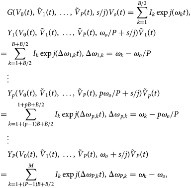
where $\tilde{V}_p\lpar t\rpar$ indicates phasors. In (8), the integer B/2 is the number of spectral lines at each side of the p-th sub-harmonic component, pf o/P, where p = 1, …, P. Thus, the total number of spectral lines is given by M = B/2 + PB. The frequency-domain models of the distributed components must be valid in the whole bandwidth of each harmonic component. For a higher P, the integration time step can, in principle, be increased as PΔt. Note that the equation at each harmonic p is analogous to the one in (2). The phasors $\tilde{V}_p\lpar t\rpar$
 , with the phases ϕp(t) = ϕo,p + Фmix,p(t), will exhibit a slower time variation for a higher P. In the limit situation P = N, the phasors $\tilde{V}_p$
 will be constant in the synchronization band. For P < N, the components $\bar{X}_k\lpar t\rpar$
 will be periodic in the locked steady state, with this time variation being due to the neighboring equally spaced spectral lines.
Unlike the envelope-domain equations (3)–(7), based on a linearization of the admittance function about the free-running solution, (8) will not be numerically resolved. In (3)–(7) the oscillator behaves linearly with respect to the K input sources, with frequencies located about the free-running one. In contrast, in (8) the oscillator will (generally) behave nonlinearly with respect to the input source at a much lower frequency. The input source plus the device nonlinearity must be able to generate a harmonic signal at the oscillation frequency, able to injection lock the oscillation. In principle, the admittance at each harmonic frequency p depends on all the harmonic voltages at the observation node, so the extraction of these admittance functions is virtually impossible. The purpose of equation (8) is to illustrate the various possible ways to partition the spectrum when analyzing the high-order sub-harmonic injection-locked oscillator with the envelope-transient method and their impact on the integration time step.
To obtain the sub-harmonic injection locking, a rectangular signal, at a frequency fo/N, is injected into the high-frequency oscillator, as shown in Fig. 2, case (ii). The rectangular signal contains a high number of harmonic terms of fo/N, which facilitates the sub-harmonic injection locking. Note that this is different from the synthesis method in [Reference Jany, Siligaris, Ferrari and Vincent1–Reference Jany, Siligaris, Ferrari and Vincent3]. In those works, a large multiplication factor is achieved by shaping the input sinusoidal signal (at low frequency), into a square signal. The shaped signal periodically switches on and off a high-frequency oscillator, suitably tuned to maximize the power at the desired harmonic terms. The resulting signal is used to injection lock a second oscillator, which enables the selection of one or another spectral line.
Here a rectangular signal is introduced into the oscillator of Fig. 2. The signal has a frequency 90 MHz, amplitude 1 Vpp, and duty-cycle of 25%. One must note that although the oscillation frequency of this prototype (2.7 GHz) is lower than the one in [Reference Jany, Siligaris, Ferrari and Vincent1–Reference Jany, Siligaris, Ferrari and Vincent3], the frequency ratio is the same N = 30, so the analysis complexity must be similar. The circuit has been analyzed with circuit-level envelope transient, following the criteria in (8), and using an AG at fo, connected to the circuit at the initial time only to initialize the oscillation, as shown in [Reference Cos, Suarez and Sancho20]. Figure 9 presents the spectrum at f out = 30 × 90MHzfor P = 1, 4, 6, which predicts a synchronized behavior. Only the central spectral lines can agree since for P > 1 part of the spectrum corresponds to terms P-1 and P + 1. For P = 1 the integration time step is 0.05 ns, whereas for P = 6 it is 0.3 ns. The analysis has been validated through an independent HB analysis (superimposed). This costly HB analysis has been carried out providing the amplitude and phase of the central spectral line, obtained with envelope transient, to an AG at f out = 30 × 90 MHz. With P = 6, the time variation is more regular, since less spectral lines contribute to this variation at each harmonic term. Thus, the synchronization bands can be determined with higher accuracy.

Fig. 9. Injection locking by a pulsed signal at 90 MHz. Output spectrum at f out = 30 × 90 MHz when considering P = 1, 4, 6. HB results are superimposed.
In this particular case (N = 30), it was possible to perform a HB simulation. Figure 10 presents the solution of the circuit in Fig. 2 when driven with a rectangular waveform of Vpeak = 1 V, frequency fin = 90 MHz and duty cycle 25%. The spectrum in Fig. 10(a) was obtained with default HB. The power of the spectral lines about the oscillation frequency (2.7 GHz) is well below that of the original free-running oscillation (7.75 dBm). Figure 10(b) presents the spectrum obtained with an AG, operating at Nfin, through the optimization of its amplitude V and phase ϕ, in order to fulfill: Y(V,ϕ) = 0. As can be seen, there is a spectral line with a much higher output power, which corresponds to the injection-locked oscillation. If the solution obtained through AG optimization is stored in an ASCII file and using it in default HB as an initial condition, the resulting spectrum is overlapped, which validates the accuracy of the AG-based procedure. By sweeping the phase ϕ and optimizing V and VD in order to fulfill: Y(V,VD) = 0, it was possible to trace the synchronization curve versus VD through AG optimization in HB [Reference Suárez10], which took approximately 3 h. The resulting closed synchronization curve (bounded by the two turning points corresponding to local/global bifurcations) is shown in Fig. 11(a). Experimental points are superimposed. The envelope-domain analysis is computationally more efficient. Figures 11(b) and 11(c) present the analysis of the synchronization band with the averaging method when considering P = 6. Figure 11(b) presents the variation of the average value of P-th harmonic component of the output voltage, 〈ϕ P(t)〉 = ϕ o,P, versus VD. which enables the detection of the locking band. Figure 11(c) presents the result of averaging the amplitude of P-th harmonic component of the output voltage, denoted as 〈V P(t)〉 = V o,P. The envelope-domain integration only provides the upper (stable) section of the synchronization curve. There is an excellent agreement with the HB predictions, though the computation time is four times shorter. Note that the comparison with HB should be performed in terms of the tuning-voltage interval with the locked operation. This is determined by the two turning points of the ellipsoidal curve, in the case of HB simulations, and the slope discontinuity, in the case of envelope-transient simulations. As can be seen, the locked-operation interval is the same as the two simulation methods.

Fig. 10. HB analysis of the circuit in Fig. 2 under a rectangular input signal of Vpeak = 1 V, frequency 90 MHz and duty cycle 25%. (a) Without AG. The oscillation is not excited. (b) With an AG, after fulfilment of the optimization condition Y(V,ϕ) = 0. The injection-locked oscillation is clearly visible. When storing the solution obtained through AG optimization in an ASCII file and using it in default HB as an initial condition, the resulting spectrum is overlapped, which validates the accuracy of the AG-based procedure.

Fig. 11. Locking band at N = 30. (a) Synchronization curve, versus VD, obtained with HB. Experimental points are superimposed. (b) Envelope-domain analysis with P = 6. Evolution of the phase average 〈ϕ P(t)〉 = ϕ o,P versus VD. (c) Evolution of the amplitude average 〈V P(t)〉 = V o,P versus VD.
Note that it was not possible to obtain any HB convergence when changing VD in order to select a different spectral line, for instance, N + 1 and N + 2. This could be easily achieved with the envelope-transient method, as shown in Figs 12(a) to 12(c), where three different spectral lines, corresponding to N = 30, N + 1 and N + 2, are selected by varying VD. Finally, the output of the subsynchronized oscillator has been connected to an analogous voltage-controlled oscillator to increase the frequency selectivity. To initialize the two individual oscillations an AG is connected to each circuit at the initial time only. The simulated spectra are shown in Figs 13(a) and 13(b). The ratio between the selected spectral line and the highest-power neighboring line is in the order of 30 dB. Figure 13(b) presents the experimental results. Similar to Fig. 7, there is a deviation in the tuning voltages, attributed to the device models.

Fig. 12. Oscillator locking to different spectral lines of the input source by tuning VD. (a) Locking to f 1 = 2.7 GHz (N = 30). (b) Locking to f 2 = 2.79 GHz (N + 1). (c) Locking to f 3 = 2.88 GHz (N + 2).

Fig. 13. Increase of the frequency selectivity through the use of a second oscillator. (a) Simulations. (b) Measurements.
Phase noise
The phase-noise analysis of the sub-harmonic injection-locked oscillator at a high order N is challenging. This is because, in most cases, the only way to obtain the steady-state solution is through an envelope-domain analysis using the criteria discussed in the section “Sub-harmonic injection -ocked operation”. Then, one faces the problem of two different time scales, in addition to the harmonic frequencies, kfo/P considered in the Fourier-series representation of the circuit variables. One of the additional time scales is slow because it is associated with the noise perturbations. The other one is faster, and depends on the P value selected in (6), which determines the bandwidth about each spectral line in the Fourier-series representation of the circuit variables. Two cases will be considered here, P = N, for which the harmonic components of the Fourier series considered in (6) take constant values, and P < N for which the harmonic components are time-varying. The case P = N will be addressed by means of a two-tier HB analysis, with the admittance function of the injection-locked oscillator at fo = Nfin constituting the outer tier. This will allow an understanding of the phase-noise response of the high-order sub-harmonic injection-locked oscillator to the noise sources. In the case P < N the key parameters determining the phase-noise response will be identified from envelope-domain simulations through a numerical procedure.
Case P = N
For P = N the sub-harmonic injection-locked oscillator will be described with an outer-tier admittance function Y extracted from HB simulations. This admittance function is similar to the one considered in the section “Oscillator injected by multiple input tones”. However, the circuit is now in injection-locked conditions with respect to the sub-harmonic source, at the high sub-harmonic order N. Thus, the function Y depends on the observation node amplitude V and phase ϕ, since the oscillation frequency is determined by the input source frequency and fulfils fo = Nfin. Thus, the synchronized solution will fulfil the following two-tier equation system:

where $\bar{H}$ represents the HB system that constitutes the inner tier, Vs and ωs are, respectively, the amplitude and phase of the steady-state solution and the vector $\bar{X}^{\prime}$
 contains all the state variables except the voltage at the observation node Ve jϕ and its complex conjugate. The above system can be solved through the optimization of V and ϕ in order to fulfil the goal Y = 0
For the noise analysis, two different contributions will be considered: the noise from the input source and the circuit own noise sources. Regarding the input source, the phase noise will be much larger than the amplitude noise, so the latter will be neglected. On the other hand, the circuit noise will be modeled with an equivalent noise-current generator at the observation node i n(t). The spectral density of this equivalent noise-current source |I N(Ω)|2is fitted with the oscillator in free-running conditions, in order to obtain the same phase-noise spectral density as with the entire set of circuit noise sources. The fitting is carried out in circuit-level HB, using the conversion-matrix approach [Reference Paillot, Nallatamby, Hessane, Quere, Prigent and Rousset30–Reference Nallatamby, Prigent, Sarkissian, Quéré and Obregón32]. The result is shown in Fig. 14. Note that in injection-locked conditions, one can expect the oscillator to follow the phase noise of the input source (usually growing as Ω3 when approaching this carrier) up to a certain (relatively high) offset frequency, above which the impact of flicker noise will usually be negligible. Thus, the fitting can be limited to the effect of the white noise sources.

Fig. 14. Fitting the spectral density of the original free-running oscillator with a single equivalent current source of spectral density |I N(Ω)|2. The fitting is carried out in circuit-level HB, using the conversion-matrix approach.
The phase noise contribution of the input source (with arbitrary waveform) will be obtained from the jitter τ(t) of this source [Reference Kaertner33, Reference Takahashi, Ogawa and Kundert34]. One must take into account that a time translation τ of the input signal gives rise to an identical time translation of the oscillator solution, which does not affect the value the admittance function Y(V s, ϕ s), depending only on the phase shift with respect to the input source. However, the time translation will modify the absolute node phase, which is increased as ϕ + Nωinτ. Thus, the jitter of the input source will give rise to the phase perturbation Nψ(t) = Nω inτ(t) at the oscillation frequency. Because there are also noise contributions coming from the oscillator circuit [modeled with the equivalent source i n(t)], the total phase perturbation of the voltage at the observation node will be Δϕ T(t) = Nω inτ(t) + Δϕ(t)where Δϕ(t) is a small increment with respect to the steady-state phase ϕo due to the noise perturbations. On the other hand, the node amplitude, under the influence of τ(t) and i n(t) becomes V s + ΔV(t).
In the presence of the noise perturbations the outer-tier system at Nωin can be obtained by performing a first-order Taylor series expansion of the total node admittance Y about the particular steady-state synchronized solution, Vs, ϕs, and ωs, which provides:

where s acts like a time differentiator and the subindexes stand for derivatives of Y with respect to the corresponding variables V, ϕ and ω, and I N(t)is the envelope of the current-noise source i n(t) about Nω s. After the time differentiation, one obtains the following equation:

where the subindexes indicate the quantity with respect to which the admittance function is differentiated. The derivatives $Y_V\comma \;Y_\omega \comma \;Y_\phi$ are calculated at the steady-state synchronized solution through finite differences in HB, following the procedure described in [Reference Ramirez, de Cos and Suarez13, Reference Ramirez, Ponton, Sancho and Suarez21].
Next, the complex equation (8) is split into real and imaginary parts and the Fourier transform is applied in the slowly varying time scale of the noise perturbations, with associated frequency Ω. Solving for Δϕ T(Ω) = Δϕ(Ω) + Nψ(Ω) and multiplying by the adjoint, the phase-noise spectral density [Reference Ramirez, Ponton, Sancho and Suarez21] is given by:

where higher-order terms in Ω have been neglected and the complex-number products of the form a × bare real and are defined as: $a \times b = {\mathop{\rm Re}\nolimits} \lpar a\rpar {\mathop{\rm Im}\nolimits} \lpar b\rpar -{\mathop{\rm Re}\nolimits} \lpar b\rpar {\mathop{\rm Im}\nolimits} \lpar a\rpar = \vert a \vert \vert b \vert \sin \lpar \angle b-\angle a\rpar$ . In turn, the angles in the third term are defined as $\alpha _{ab} = \angle b-\angle a$
 . To derive the above expression, it has been taken into account that the real and imaginary parts of the equivalent noise source $\bar{I}_N$
 are uncorrelated and the input noise is uncorrelated with the oscillator noise. Dividing the numerator and denominator by $\vert {Y_{\rm V} \times Y_\phi } \vert ^ 2$
 , one obtains:

which can be rewritten as:

where the following parameters have been introduced:

As gathered from (14), the injection-locked oscillator exhibits a low-pass response with respect to the input phase noise and its own noise sources, with a 3 dB cut-off frequency ω 3dB. As shown in (15), the corner frequency ω3dB will be, in principle, smaller for a higher quality factor of the oscillator (larger $\vert {Y_\omega } \vert$ ) and larger for a higher $\vert {Y_\phi } \vert$
 , implying a higher sensitivity to the input source and thus a larger locking range. Note, however, that the angles α Vϕ, α Vω can be very relevant.
For small offset frequency, the phase noise follows N 2|ψ(Ω)|2, as derived from the jitter τ(t) of the input signal. The effect of the circuit noise sources is determined by $A_p\vert {I_N} \vert ^2/V_s^2$ . If $A_p\vert {I_N} \vert ^2/V_s^2 \gt N^2\vert {\psi \lpar \Omega \rpar } \vert ^2$
 from a certain Ω < Ω3B, before decaying −20 dB/dec.
The predictions of the semi-analytical expression (14) have been compared with a phase-noise analysis of the sub-harmonic injection-locked oscillator at N = 30, performed in HB, with the conversion-matrix approach [Reference Paillot, Nallatamby, Hessane, Quere, Prigent and Rousset30–Reference Nallatamby, Prigent, Sarkissian, Quéré and Obregón32]. The results of this comparison, in the presence of the equivalent white-noise source i n(t), are shown in Fig. 15. The curves providing the phase-noise spectral density obtained with the two methods are overlapped. Remember that the spectral density of the white-noise source |I N|2 was fitted in the standalone free-running oscillator. The corner frequency is f 3 dB ≅ 1.5 MHz.

Fig. 15. Comparison of the results of the semi-analytical expression (14) and the conversion-matrix approach when only white-noise sources are considered. Note that the spectral density of the white-noise source |I N|2 was fitted in the standalone free-running oscillation.
For the prediction of the whole spectrum, the phase noise of the rectangular input source at the fundamental frequency (90 MHz) has been experimentally characterized, using the R&S FSWP8 – Phase Noise Analyzer, and introduced in (14). Figure 16 presents a comparison of the predictions from (14) with the experimental measurement of the oscillator phase at Nfin. Note that there is an excellent agreement since the two curves are nearly superimposed. At the lower offset frequencies, the phase noise is 20log(30) higher than the one at the lower harmonic frequency of the input source, included in the figure. The phase-noise spectrum in free-running conditions is also shown for comparison. The spectrum of the injection-locked oscillator follows the input-noise source up to its corner frequency f 3 dB ≅ 1.5 MHz. Up to this frequency, there is a negligible effect of the circuit own noise sources. At low-frequency offset, there is an improvement of more than 30 dB. To obtain a lower spectral density at higher offset frequencies an input source with lower phase noise should be used.

Fig. 16. Comparison of the predictions from (14) with the experimental measurement of the oscillator phase at Nfin. At the lower offset frequencies, the phase noise is 20log(30) higher than the one at the lower harmonic frequency of the input source, included in the figure. The phase-noise spectrum in free-running conditions is also shown for comparison.
Case P ≤ N
For P < N the quantities $A_p/V_s^2$ and Ω3 dB, will be identified from envelope-domain simulations through a numerical procedure. To obtain the frequency response of the oscillator phase with respect to the equivalent noise source |I N|2, this noise source will be replaced with a deterministic tone at the frequency Ω. Then, a two-tone envelope-domain analysis will be carried out, using the frequency basis (ω 1 = ω o/P, ω 2 = Ω). Then, for each Ω, the phase shift will be calculated from the voltage spectrum at the observation node [Reference Ramirez, Ponton, Sancho and Suarez21], doing:

To obtain the voltage components in the above expression, the time-varying harmonic components resulting from the envelope-domain analysis can be processed to provide:

where the operator 〈 〉 applies an averaging in the period T in = 1/f in and X k,l(t) is the harmonic component corresponding to the frequency kω 1 + lω 2. Note that the time-varying nature of the harmonics X k,l(t) is due to the presence of frequency components at multiples of the injection frequency f in, which are removed by the operator 〈 〉. Sweeping Ω and tracing |Δϕ(Nω in + Ω)|2 versus Ω one obtains a frequency response from which one can identify the two quantities $A_p/V_s^2$ and Ω3 dB. Once these quantities are available, one can obtain the phase-noise spectrum through (17).
Conclusion
A methodology for the analysis of sub-harmonically injection-locked oscillators under a high order N has been presented. This analysis is involved since harmonic-balance will not be applicable in most cases due to the need to fulfil the injection-locked oscillation condition under a high number of harmonic terms. Instead, an envelope-domain analysis has been proposed here. The procedure has been initially derived and tested in the case of an oscillator injected by a number of closely spaced input tones. In these conditions, the oscillator is described with the aid of a semi-analytical formulation, based on the modeling of this oscillator with an outer-tier admittance function extracted from harmonic-balance simulations. The locking bands about each of the input tones, obtained when sweeping a tuning voltage, can be efficiently predicted by averaging the phase of the integrated solution. This procedure has been extended to the more demanding case of a sub-harmonic injection-locked oscillator, simulated through a circuit-level envelope transient. The phase noise of the sub-harmonic injection-locked oscillator has been analyzed with a semi-analytical formulation, based on an admittance model of the oscillator circuit in injection-locked conditions. The effect of the phase noise of an arbitrary periodic input waveform has been derived from its associated timing jitter. The analytical expression for the phase-noise spectral density shows that the injection-locked oscillator exhibits a low-pass response with respect to the noise sources. It initially follows N times the phase noise of the fundamental frequency of the input-source and then follows its own input noise sources. The procedure has been illustrated with a practical FET-based sub-harmonic-injection-locked oscillator at the order N = 30.
Acknowledgements
This work was supported by the Spanish Ministry of Science, Innovation and Universities and the European Regional Development Fund (ERDF/FEDER) under the research project TEC2017-88242-C3-1-R.
 Silvia Hernández was born in the Canary Islands, Spain. She received her M.S. degree in Telecommunication Engineering from the University of Las Palmas de Gran Canaria, Canary Islands, Spain, in 2015. The same year, she entered the Institute for the Technological Development and Innovation in Communications, University of Las Palmas de Gran Canaria, as a research assistant. In 2016, she joined the Communications Engineering Department, University of Cantabria, where she is currently working towards her Ph.D. degree. Her research interests include stability analysis and the study of new methods for the analysis and design of nonlinear microwave circuits.
 Mabel Pontón was born in Santander, Spain. She received the bachelor's degree in telecommunication engineering, master's degree in information technologies and wireless communications systems, and Ph.D. degree from the University of Cantabria, Santander, in 2004, 2008, and 2010, respectively. In 2006, she joined the Communications Engineering Department, University of Cantabria. From 2011 to 2013, she was with the Group of Electronic Design and Applications, Georgia Institute of Technology, Atlanta, GA, USA, as a Post-Doctoral Research Fellow. Her current research interests include the nonlinear analysis and simulation of radiofrequency and microwave circuits, with an emphasis on phase-noise, stability, and bifurcation analysis of complex oscillator topologies.
 Sergio Sancho received the degree in Physics from Basque Country University in 1997. In 1998 he joined the Communications Engineering Department of the University of Cantabria, Spain, where he received the Ph.D. degree in Electronic Engineering in February 2002. At present, he works at the University of Cantabria, as an Associate Professor of its Communications Engineering Department. His research interests include the nonlinear analysis of microwave autonomous circuits and frequency synthesizers, including stochastic and phase-noise analysis.
 Almudena Suárez was born in Santander, Spain. She received the degree in electronic physics and the Ph.D. degree from the University of Cantabria, Santander, Spain, in 1987 and 1992, respectively, and the Ph.D. degree in electronics from the University of Limoges, France, in 1993. At present, she is a Full Professor at the University of Cantabria and a member of its Communications Engineering Department. She has authored the book Analysis and design of autonomous microwave circuits for the publisher IEEE–Wiley and co-authored the book Stability analysis of microwave circuits for the publisher Artech–House. She belongs to the technical committees of the IEEE International Microwave Symposium and European Microwave Conference. She was an IEEE Distinguished Microwave Lecturer for the period 2006–2008. She is an associate editor of the IEEE Microwave Magazine. She is a member of the Board of Directors of EuMA and the Editor in Chief of International Journal of Microwave and Wireless Technologies from Cambridge University Press.


