1. Introduction
Joints that are opening-mode fractures are the most common geological structures in the Earth's crust, and their spacing is important for many applications. Geologically, Naylor & Stephenson (Reference Naylor and Stephenson2010) showed that significant differences in joint spacing, persistence of discontinuities and block size were correlated to mesoscale erosion in Australian and Welsh study sites. Stephenson & Naylor (Reference Stephenson and Naylor2011) demonstrated that the shape and size of boulders, liberated from layers of Blue Lias Limestone in Wales, United Kingdom, could be linked to the thickness of beds and joint spacing. Joint spacing is important in rock mechanics, as demonstrated by Storti et al. (Reference Storti, Balsamo, Cappanera and Tosi2011), who found that its variability is associated with the weakening of bedding in chalk atop of the Krempe salt ridge at Lägerdorf, NW Germany. Joint spacing is also significant in engineering projects. Brown et al. (Reference Brown, DuTeaux, Kruger, Swenson and Yamaguchi1999) found that fluid circulation and production temperature in engineered geothermal reservoirs, particularly the Hot Dry Rock system, depends on the mean effective joint spacing. For the construction of a breakwater to be economical as well as effective, prediction of in situ block sizes from joint spacing data is a vital early design input (Latham, Meulen & Dupray, Reference Latham, Meulen and Dupray2006). In tunnel engineering, there are strong relationships between geological parameters like joint spacing and tunnel boring machine (TBM) performance parameters (Hassanpour, Rostami & Zhao, Reference Hassanpour, Rostami and Zhao2011). Joint spacing often provides basic information in hydrology, oil and gas industries, material engineering and more (Bahat, Rabinovitch & Frid, Reference Bahat, Rabinovitch and Frid2005).
Commonly, joint spacing is examined under conditions of layer-parallel extension under constant layer-normal stress. A good review can be found in Shöpfer et al. (Reference Schöpfer, Arslan, Walsh and Childs2011). It is usually claimed that fracture spacing increases with layer thickness (e.g. Ladeira & Price, Reference Ladeira and Price1981). A consequence of this scaling is sequential infilling: new fractures forming between existing fractures (Bai & Pollard, Reference Bai and Pollard2000 b). Sequential infilling by all shear lag models (Cox, Reference Cox1952; Hobbs, Reference Hobbs1967) favours mid-way fracturing between existing fractures (Ohsawa et al. Reference Ohsawa, Nakyama, Miwa and Hasegawa1978; Schöpfer et al. Reference Schöpfer, Arslan, Walsh and Childs2011). Fracture saturation is assumed to occur when a critical ratio of fracture spacing to thickness is reached (see Section 3.a below). A possible obstacle for joint propagation and hence for saturation is suggested by Bai & Pollard (Reference Bai and Pollard2000 a) to be a layer-parallel compressive normal stress arising between existing joints. A typical outcrop of intensively jointed sedimentary formation with a close-up view of a fractured limestone bed is shown in Figure 1. We use this exposure, by Becker & Gross (Reference Becker and Gross1996), in our joint spacing analysis in Section 3.b below. Jain, Guzina & Voller (Reference Jain, Guzina and Voller2007) calculated the stress profile in a competent layer as a function of the distance from an existing joint. The calculation shows that a one-dimensional approach (similar to that of Cox, Reference Cox1952 and Hobbs, Reference Hobbs1967) is quite sufficient in obtaining a very accurate approximation to the more elaborate 2D procedure (e.g. Bai & Pollard, Reference Bai and Pollard2000 a,b). Jain, Guzina & Voller (Reference Jain, Guzina and Voller2007) included in their method the influence of both the overburden and the possibility of slip between the competent and the adjacent layers.

Figure 1. The studied bed and the definitions of bed boundaries, bed thickness and spacings (adapted from Becker & Gross, Reference Becker and Gross1996).
In this paper we deal with the statistical considerations of the build-up of the joint spacing distribution, which were not treated in Jain, Guzina & Voller (Reference Jain, Guzina and Voller2007). Since we are interested in presenting the basic features of the phenomenon, we use here the simplest ‘shear lag’ result, namely that of Hobbs (Reference Hobbs1967), for the stress profile away from an existing joint. Inclusion of slip and/or overburden or using other stress field models (such as that of Bai & Pollard, Reference Bai and Pollard2000 a,b) can easily be accommodated in our approach by changing Eq. (2) below or by using the appropriate model's numerical results in Eq. (2). The use of just the simple Hobbs (Reference Hobbs1967) model is shown to be adequate to describe field results of joint spacing quite reliably. Furthermore, the overburden effect can sometimes be compensated for by the ‘Secor effect’ (Secor, Reference Secor1965, Reference Secor1969).
We postulate here that the criterion for fracture for the jointed layers is really based only on the level of stress (σ) that they have endured during the elapsed geological time. This is founded on the assumption that the flaw distribution is unvarying across the bed. It is conceivable that such a fracture criterion based on σ alone is the prevailing one for sub-critical (below KIc) extended-time fractures for all brittle materials. This result is shown to be in line with results obtained in experiments on ‘lengthy’ laboratory creep (Yoon, Wiederhorn & Luecke, Reference Yoon, Wiederhorn and Luecke2000). Note that we are dealing only with joints that were formed quasi-statically, not with joints cutting granites, which occasionally are proven to be dynamic (above KIc). It is observed that dynamic joints are relatively abundant in granites whereas quasi-static ones are prevalent in sedimentary rock layers (Bahat, Bankwitz & Bankwitz, Reference Bahat, Bankwitz and Bankwitz2003).
Joint spacing in layered rocks is considered to have originated by two main processes, and possibly by intermediate ones.
The first process envisages the layer denoted by A, as being ‘sandwiched’ by two, ‘upper’ and ‘lower’, neighbouring layers (see Fig. 1), each of which is made of different material to that of A. The neighbouring layers, because of their higher compliance, are usually less jointed than A. But they tend to stretch the latter when they themselves are stretched, thus transferring the stress to it. This process is referred to as the Cox–Hobbs case after the two authors who analysed it (Cox, Reference Cox1952; Hobbs, Reference Hobbs1967). In this process the three layers are treated as perfectly connected (glued) to each other, and the shear stress transferred at the inter-layers is transposed into tensile stress in the middle layer. The Cox–Hobbs model can be divided into two parts. The first part, based on Cox (Reference Cox1952), calculates the stress transfer from the outer layers to A, and the second part treats the process of joint ‘infilling’, i.e. the addition of more and more fractures to the layer, as a function of strain (or stress) increase.
The second process by which a layer is stretched and jointed is when it is completely separated from its neighbouring layers and is itself pulled upon, either by remote tectonic stresses or by pore pressure, or both. This process is called the Pollard–Segall model (Pollard & Segall, Reference Pollard, Segall and Atkinson1987) after the two authors who analysed it.
These two end-member processes of layer fracturing actually appear in nature, as do intermediate modes in which the ‘gluing’ of the layers is less than absolute and friction exists between the A layer and its neighbours, thus transferring to A only part of the stress in them. Jain, Guzina & Voller (Reference Jain, Guzina and Voller2007) calculated a partial transfer of stress by treating the possibility of slip between the layers.
1.a. Basic terms
Shadow: An important physical term related to joint spacing is the shadow zone (Rives et al. Reference Rives, Razack, Petit and Rawnsley1992; Rabinovitch & Bahat, Reference Rabinovitch and Bahat1999). The term shadow zone used in the literature describes a region around an existing joint in which no new joints can occur (e.g. Rives et al. Reference Rives, Razack, Petit and Rawnsley1992), generally also termed an opaque shadow zone. A non-opaque shadow zone would entail the possibility of additional joints appearing in this region but only under very stringent conditions (very high stresses, Rabinovitch & Bahat, Reference Rabinovitch and Bahat1999). Figure 2 depicts (schematically) two joint spacing distributions for an opaque and non-opaque shadow zone, respectively.
Figure 2. Schematic joint spacing distribution under opaque and non-opaque shadow conditions. Each distribution contains zero frequency at zero and a very high spacing and a peak at the most frequent spacing. The opaque shadow distribution includes a zero joint spacing region where no fractures appear.
Saturation: This is another term used to describe the jointing phenomenon. Thus, in relation to opaque shadow, there is a complete saturation in the total number of fractures inside a layer (demonstrated, for example, by the lack of joints in the first part of the joint spacing of the opaque shadow part of Fig. 2); whereas in relation to non-opaque shadow, saturation is only an apparent saturation in which the addition of joints to the layer requires larger and larger amounts of additional strain.
Slow phenomena: We are considering here very slow phenomena, which no laboratory measurements can exactly simulate. The experiments that have the closest similarity to them are those related to creep or fatigue (e.g. creep experiments can last up to ~ 1 year). The durations of both experiment types are of course much smaller than geological ones. Nevertheless, we shall use results of a creep experiment to glean some information about geological jointing.
Flaw distribution: There are several ways in which to describe the flaws in the material, which, under stress, lead to the development of joints. The simplest one is to state the distributions of flaws according to their size and to the angle to the existing stress field. A different method is to directly state the flaw cumulative distribution function according to their strength, namely the probability that (under a specific stress field) a flaw would turn into a joint at or above a specific stress value. Note that for regular engineering experiments this limiting value is connected with the probability that the KI value at the tip of this flaw reaches KIc; while for creep or subcritical experiments, the attainment of a lower value of KI, denoted by KI0 (Wan, Lathabai & Lawn, Reference Wan, Lathabai and Lawn1990), is implied. That is, for the latter experiments a shift of the distribution to lower values of stress is indicated.
2. The model
The model consists of two components, the statistical part and the value of the stress field around an existing joint. The statistical part is similar to the one introduced in Rabinovitch & Bahat (Reference Rabinovitch and Bahat1999) but here, the stress field used is the Cox–Hobbs ‘shear lag’ theory and an analytical solution is obtained. We use here an approximation, strictly applied only to joint densities that are not too large, since no account is taken of the lowering of the inter-joint maximal stress value. On the other hand, since it provides a good approximation to the fracturing processes at short distances from existing fractures, it can probably be used also for large joint densities.
2.a. The statistical part
The statistical part is based on the distinction between two properties. The first, q(x)dx (see Fig. 3), is the probability that a new fracture would occur in between a distance x and a distance x+dx from an existing joint. The second, p(ℓ)dℓ (Figs 2, 4, 5), is the probability that an additional fracture would appear between distances ℓ and ℓ+dℓ from an existing joint and no other fracture has occurred up to distance ℓ. This distinction is analogous to the following two probabilities of coin flipping. The first, q, is analogous to the probability (1/2) of getting heads in the fifth, say, throw of the coin, while the second, p, is analogous to the probability that the outcome of the fifth throw would be heads when all four previous throws were tails. Heads and tails correspond to fracture and no-fracture, respectively. Obviously, p < q. Note that the measured histograms in the literature are proportional to p(ℓ). Our approach is compared to the Weibull distribution, based on the weakest link theory, in Appendix 1.

Figure 3. The assumption that q(x) is proportional to σ. (a) σ(x) according to the Cox–Hobbs model. σ0 – the remote stress. (b) q(x) = γσ(x) (full line) and an opaque shadow q(x) (dashed line).

Figure 4. Division of ℓ into N intervals of length dx each. p(ℓ) measures the probabilities that no fracture has occurred between 0 and ℓ, and that the first new fracturing did take place at ℓ.

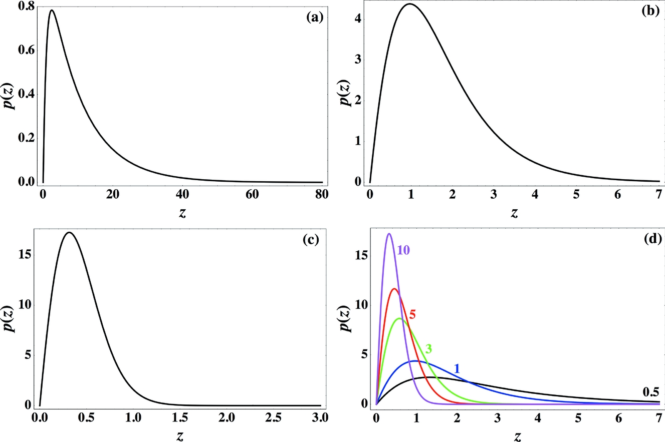
Figure 5. Theoretical spacing distributions, p(z) (arbitrary units), for the Cox–Hobbs case (Eq. 1). Lengths z are measured in dimensions of δ: z = ℓ/δ. (a) For η = 0.1, (b) for η = 1.0, and (c) for η = 10.0. Note that η is proportional to the remote stress in the layer and to δ. (d) For η = 0.5, 1, 3, 5, 10; here distributions are shown on the same scale to emphasize the fast change of the peak with η between 0.5 and 3 and the slow change for η between 5 and 10.
2.b. The stress field part
Regarding the stress field, we concentrate here on the ‘shear lag’ Cox–Hobbs case, which is relevant, for example, to the field observations by Becker & Gross (Reference Becker and Gross1996). As mentioned in Section 1 above, other models, such as that of Bai & Pollard (Reference Bai and Pollard2000 a, b) can be used as well within the framework of the statistical part. In the absence of slip (or debonding) between the layers, the ‘shear lag’ theory predicts that the stress ‘recovery’, σ(x), in the fracturing layer as a function of the distance x away from an existing fracture (Fig. 3), behaves (Hobbs, Reference Hobbs1967, eq. (7)) like:
 \begin{equation}
\sigma (x) = \sigma _0 [1 - \exp \,(- \left| x \right|/\hbox{\idel})]\end{equation}
\begin{equation}
\sigma (x) = \sigma _0 [1 - \exp \,(- \left| x \right|/\hbox{\idel})]\end{equation}
Note that Eq. (1) is an approximation, valid when the number of joints is not too large (see Section 5 below).
All of our results are based on one assumption: the probability of a crack forming at a distance x (q(x), Fig. 3) from an existing fracture in a rock layer is proportional to the tensile stress σ at x. We regard the agreement between measured distributions in the field and the results obtained here (see Section 3 below) to be a good indication of the validity of our assumption. Note that we do not assume any lower value of σ, such as a rock strength, below which no fracture could occur, since we consider the possibility of large enough flaws that could have appeared during the geological times discussed here, and would lead to fracture even at very low stresses.
2.c. The combined model
Thus, let q(x)dx be the probability that an additional fracture appears between x and x + dx (Fig. 3a). We assume that q(x) = γσ(x) where γ is a proportionality constant. This assumption is evidently based on the presumption that the flaw density is unchanged along the bed. Hence we posit (Fig. 3b), by Eq. (1),
 \begin{equation}
q(x) = \gamma \sigma _0 \,[1 - \exp \,(- \left| x \right|/\hbox{\idel})]\end{equation}
\begin{equation}
q(x) = \gamma \sigma _0 \,[1 - \exp \,(- \left| x \right|/\hbox{\idel})]\end{equation}
Now define p(ℓ)dℓ to be the probability that the distance between neighbouring joints would reside exactly in the interval between the distance ℓ and the distance ℓ+dℓ (Rabinovitch & Bahat Reference Rabinovitch and Bahat1999, see also Section 2.a). The probability p(ℓ)dℓ is equal to the product of two terms. First, the probability y(ℓ) that no fracture has occurred between x = 0 and x = ℓ, and second, the probability that it actually did occur between x = ℓ and x = ℓ+dℓ. The second probability is of course q(ℓ)dℓ, while the first one is somewhat more difficult to obtain. Let us divide ℓ into N intervals each of length dx = ℓ/N (Fig. 4). As mentioned, the probability of an additional fracture appearing in dx at a distance x from the origin (where a crack resides) is just q(x)dx. Therefore, the probability that no crack appears in dx is (1 − q(x)dx). Since the probabilities in all intervals are mutually independent the probability that no fracture has appeared in all N intervals is the product, denoted by ∏ N i=1, of the individual ones, namely
 \begin{equation}
y(\ell) = \prod\limits_{i = 1}^N {\,[1 - q(x_i)\,dx]}\end{equation}
\begin{equation}
y(\ell) = \prod\limits_{i = 1}^N {\,[1 - q(x_i)\,dx]}\end{equation}
 \begin{equation}
{\rm ln}\,y(\ell) = \sum\limits_{i = 1}^N {{\rm ln}\,[1 - q(x_i)\,dx]}\end{equation}
\begin{equation}
{\rm ln}\,y(\ell) = \sum\limits_{i = 1}^N {{\rm ln}\,[1 - q(x_i)\,dx]}\end{equation}
Passing to the limit as dx → 0 we get
 \begin{equation}
\mathop {\lim}\limits_{\scriptstyle dx \to 0 \atop
\scriptstyle N \to \infty} \quad {\rm ln}\,y(\ell) = - \int_0^\ell {q(x)\,dx}\end{equation}
\begin{equation}
\mathop {\lim}\limits_{\scriptstyle dx \to 0 \atop
\scriptstyle N \to \infty} \quad {\rm ln}\,y(\ell) = - \int_0^\ell {q(x)\,dx}\end{equation}
 \begin{equation}
\frac{{\lim}}{{\varepsilon \to 0}}\quad {\rm ln}\,\left| {1 - \varepsilon} \right| = - \varepsilon\end{equation}
\begin{equation}
\frac{{\lim}}{{\varepsilon \to 0}}\quad {\rm ln}\,\left| {1 - \varepsilon} \right| = - \varepsilon\end{equation}
 \begin{equation}
p(\ell) = q(\ell)\exp \left\{- \int_0^\ell {q(x)\,dx} \right\} .\end{equation}
\begin{equation}
p(\ell) = q(\ell)\exp \left\{- \int_0^\ell {q(x)\,dx} \right\} .\end{equation}
 \begin{equation}
\int_0^\infty {p(\ell)\,d\ell} & = & \int_0^\infty {\frac{{du(\ell)}}{{d\ell}}} \exp (- {u})\,d\ell \nonumber\\
& = & \int_0^\infty {\exp \,(- {u})\,du = 1}\end{eqnarray}
\begin{equation}
\int_0^\infty {p(\ell)\,d\ell} & = & \int_0^\infty {\frac{{du(\ell)}}{{d\ell}}} \exp (- {u})\,d\ell \nonumber\\
& = & \int_0^\infty {\exp \,(- {u})\,du = 1}\end{eqnarray}
 $q(\ell) = \frac{{du(\ell)}}{{d\ell}}$
and
We establish our proposed relation, q = γσ in two ways. First, we assume this relation to hold, and calculate the exact p(ℓ) that should arise. This procedure is carried out for the Cox–Hobbs case, and the results are compared with the field data of Becker & Gross (Reference Becker and Gross1996). Agreement between the model and the experimental distributions obtained there is quite good. The model also readily explains the ‘closely spaced fractures’ appearing in Becker & Gross (Reference Becker and Gross1996) for which Bai & Pollard (Reference Bai and Pollard2000
b) invoked an additional mechanism (flaw size, length and position distribution, possible pore pressure). The second verification of the q(x) = γσ(x) relation is derived from an extended creep experiment of Yoon et al. (Reference Yoon, Wiederhorn and Luecke2000), which agrees with this relation for low σ values.
$q(\ell) = \frac{{du(\ell)}}{{d\ell}}$
and
We establish our proposed relation, q = γσ in two ways. First, we assume this relation to hold, and calculate the exact p(ℓ) that should arise. This procedure is carried out for the Cox–Hobbs case, and the results are compared with the field data of Becker & Gross (Reference Becker and Gross1996). Agreement between the model and the experimental distributions obtained there is quite good. The model also readily explains the ‘closely spaced fractures’ appearing in Becker & Gross (Reference Becker and Gross1996) for which Bai & Pollard (Reference Bai and Pollard2000
b) invoked an additional mechanism (flaw size, length and position distribution, possible pore pressure). The second verification of the q(x) = γσ(x) relation is derived from an extended creep experiment of Yoon et al. (Reference Yoon, Wiederhorn and Luecke2000), which agrees with this relation for low σ values.
3. Model implications
3.a. General
For the Cox–Hobbs case, we insert in Eq. (7) the form of q(x) of Eq. (2) and obtain:
 \begin{equation}
p(\ell) = ({\rm \eta}/\hbox{\idel})\,[1 - \exp \,(- z)]\exp \,\{- {\rm \eta}\,[z - 1 + e^{- z} ]\}\end{equation}
\begin{equation}
p(\ell) = ({\rm \eta}/\hbox{\idel})\,[1 - \exp \,(- z)]\exp \,\{- {\rm \eta}\,[z - 1 + e^{- z} ]\}\end{equation}
 \begin{eqnarray}
p(\ell) &=& {\rm \gamma}\sigma _0 [1 - \exp (- \ell /\hbox{\idel})]\nonumber\\ &&\times\exp \{- {\rm \gamma}\sigma _0 [\ell - \hbox{\idel} \,(1 - \exp \,(- \ell /\hbox{\idel})]\}\qquad
\end{eqnarray}
\begin{eqnarray}
p(\ell) &=& {\rm \gamma}\sigma _0 [1 - \exp (- \ell /\hbox{\idel})]\nonumber\\ &&\times\exp \{- {\rm \gamma}\sigma _0 [\ell - \hbox{\idel} \,(1 - \exp \,(- \ell /\hbox{\idel})]\}\qquad
\end{eqnarray}
(1) Lengths are always measured in units of δ = (d/2) (E/GN)1/2. The latter has units of length and, in a sense, normalizes bed thicknesses. Normalized spacing z = ℓ/δ can then be compared between different beds.
(2) The proportionality constant, γ(= q/σ), has units of length*(stress)−1 or units of (surface tension)−1. It can probably be deduced from creep experiments (see Section 4 below) if the latter can be seen as applicable to geological processes.
(3) The parameter η = γσ0δ is dimensionless. A crude interpretation of it is that it provides the approximate probability that a second crack would appear within a distance δ of an existing fracture. Higher η values therefore imply higher joint densities.
(4) The parameter γσ0(= η/δ) has dimensions of (length)−1. It measures the probability per unit length that a second crack appears a long distance away from an existing fracture. As such it is a direct measure of joint density.
(5) It is seen that the only genuine length-normalizing coefficient is δ, being the inherent physical variable of the Cox–Hobbs spacing. Nevertheless, regarding the question of the addition of distributions from different layer positions and different lithologies, it is clear (from Fig. 5) that such a procedure is not advisable. For example, an addition of two, even normalized distributions of types 5a and 5c, say, would create a ‘distribution’ having a fictitious double peak.
Eq. (9) can be viewed as the one and only joint spacing distribution, both for low and (not too) high densities of joints. It is thus not a transition between exponential, log normal to normal distributions (Rives et al. Reference Rives, Razack, Petit and Rawnsley1992). The exact distribution, Eq. (9), is shown in Figure 5 for several joint densities. The latter are represented by the parameter η. Note that the shapes of these distributions could easily mislead one to assume that the formerly mentioned transitions do occur.
At this point we derive some features of the distribution (Eq. 9a) and discuss the significance of the only two parameters that appear therein, namely δ and η. First, let us remark that since all lengths are scaled by δ, any measured statistic such as the average or the median should also be proportional to δ. We next discuss the behaviour of the distribution median, its peak and the related interesting question of joint ‘saturation’.
We start with the question of what ‘saturation’ is and what is its origin. Saturation (see Section 1.a) arises by the following two opposing influences. On the one hand, a larger stress results in smaller joint spacing. On the other hand, an opaque shadow prohibits spacing from going to zero, namely there is a certain maximum number of joints in a layer. Experimental results, however, show ‘closely spaced fractures’ (see e.g. Bai & Pollard, Reference Bai and Pollard2000 b). To understand the real solution of this quandary, consider Eq. (9) and Figure 5d. It is seen that the distribution becomes more and more concentrated as η (or σ0) increases. Yet, the positions of the peak and the mean of the distribution only slightly decrease with η, and it seems that they would never become zero. Actually, as σ increases, the additional amount of stress needed for the same incremental decrease in spacing greatly increases. It costs more, in terms of σ, to create a new crack. To calculate the position of the peak of the distribution as a function of η, we equate to zero the derivative of p(ℓ) with respect to ℓ. This yields exp (−z)−η(1−exp (−z))2=0 or, denoting ν = exp (−z) and solving for the quadratic equation, we get
 \begin{equation}
{\nu} = 1 + 1/(2{\rm \eta}) \pm (1/{\rm \eta} + 1/(4{\rm \eta}^2))^{1/2}\end{equation}
\begin{equation}
{\nu} = 1 + 1/(2{\rm \eta}) \pm (1/{\rm \eta} + 1/(4{\rm \eta}^2))^{1/2}\end{equation}
 \begin{equation}
z_{\max} = - {\rm ln}\,[1 + 1/(2{\rm \eta}) - (1/{\rm \eta} + 1/(4{\rm \eta}^2))^{1/2} ]\quad \end{equation}
\begin{equation}
z_{\max} = - {\rm ln}\,[1 + 1/(2{\rm \eta}) - (1/{\rm \eta} + 1/(4{\rm \eta}^2))^{1/2} ]\quad \end{equation}

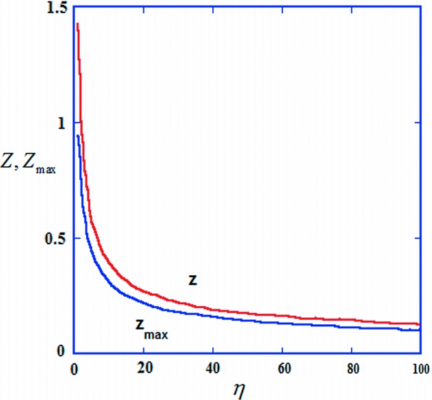
Figure 6. Distribution peaks, Z max, and medians Z (both measured in dimensions of δ) as functions of η. Note the fast change of Z max and Z values for small η values, where new cracks are relatively easy to form for even a small change of stress, and the very slow (logarithmic) change of these values for larger η (effective saturation) where increasing the crack density becomes harder and harder.
The median of the distribution ℓ = δZ can easily be calculated numerically. Results are shown in Figure 6 where Z is shown as a function of η. It is seen that the behaviour of the median is similar to that of the mean, as expected. Since Z = ℓ/δ, which is proportional to ℓ/d, Z is actually proportional to the FSR parameter (Gross, Reference Gross1993) (called by Bai & Pollard (Reference Bai and Pollard2000 a, b) the ‘fracture spacing to layer thickness ratio’). The parameter Z is (within Cox–Hobbs's model) the ‘correct’ normalized fracture spacing ratio. If Z would have been a constant, then the slope of ℓ as a function of d (more accurately as a function of δ) would have been constant, leading to a constant value of the FSI (fracture spacing index; Narr & Suppe, Reference Narr and Suppe1991), which is the slope of the best fit line for points depicting ℓ v. d for layers of different thicknesses. According to Figure 6 this is not so. The median is proportional to δ only as long as η does not change significantly between different layers. This implies that the straight line obtained for FSI measurements from different layers (Narr & Suppe, Reference Narr and Suppe1991) is somewhat fortuitous. For an ‘almost exact’ linear dependence, both σ0 and δ would have to be the same for the different layers, the spread of layer thickness for the different layers should not be too large and should lie in the larger η (‘effective saturation’) region.
This study shows that there are only two parameters that can be obtained by the analysis of spacing distributions, i.e. δ and η (or δ and γσ0). The value of δ can also be calculated by the layer thickness and the elastic properties of the rock; therefore, η becomes the most important measurable parameter. Its value, (a) determines the position of the fracture population of a particular layer with respect to effective saturation, and (b) on comparing different layers, can provide ratios of remote stresses causing fracture in them. It is seen (Figs 5, 6) that spacing distribution depends on the maximum stress that has acted in the rock layer for a significant period of time.
3.b. Comparison with jointing in nature
We now show that the distribution of Eq. (9) is indeed compatible with the histograms of joint spacing measured by Becker & Gross (Reference Becker and Gross1996, fig. 9; see our Fig. 7) of the Turonian Gerofit Formation (Fig. 1), southern Israel. The comparison is itemized here for their section I, and calculated results of all sections are given subsequently.

Figure 7. Joint spacing distributions of the Turonian Gerofit Formation, South Israel (adapted from Becker & Gross, Reference Becker and Gross1996, fig. 9).
3.b.1. Compatibility
The ℓ axis for section I stretches between 0 and 80 cm, in increments of 3 cm. The bars have heights (number of points) as follows 1, 4, 9, 14 . . . (Fig. 7I). Since we would like to treat unit length increments of 1 cm each, each bar should actually appear three times and be of one-third height. The sum of all bin heights is 110. In order that the distribution be normalized (the sum of all bin heights be equal to one) each number should be divided by 3 × 110 = 330. The numbers thus obtained (Fig. 8a) are compared to Eq. (9b) in a ‘least square’ fashion (such as ‘curve fit’ in Matlab). Here, the two parameters sought are γσ0 and δ. Results for all four sections are shown in Figure 8 and the values of γσ0, δ and η = γσ0δ are summarized in Table 1.

Figure 8. Analysis of results of Becker & Gross (Reference Becker and Gross1996) spacing measurements. Sections I–IV are given in (a–d), respectively. * are measurements and full lines are fits (Eq. (9)). Note that spacing (ℓ, measured in centimetres) is not normalized to δ but p(ℓ) is normalized (see text).
Table 1. Physical parameters of joint spacing (based on data from Becker & Gross, Reference Becker and Gross1996)

As seen, the agreement of the data to Eq. (9b) is very good, especially the shapes of the distributions. Note that the existing scatter of points in Figure 8a and 8d, is derived from the relatively small number of measurements in these cases, 110 and 94, respectively, and the spacing range over which these measurements extended was relatively large (0–80 cm), compared with Figure 8b, c, which shows far less scatter because the number of measurements were 237 and 271, respectively, and the spacing range covered only 0 to ~ 40 cm. Moreover, the scatter in Figure 8a, d is very evenly distributed around the computed distribution, rendering it to be of a random error type rather than a cause of doubt in the distribution shape itself.
The values of η obtained for sections I, III and IV are all around 1.5, placing these sections deep inside the ‘unsaturated’ region in Figure 6. The high η value of section II indicates that this section has ‘suffered’ a much higher stress (strain) during its history, bringing it (or at least the IIb part) into the saturated region.
A simple test of the self-consistency of the results can be carried out. Consider, for example, section III. A direct measurement from the histogram yields the median to be ℓ ≈ 11.5 cm, hence, Z = ℓ/δ ≈ 11.5/11.37 = 1.01. From Figure 6 this Z value leads to η ≈ 1.7, which is close to the 1.41 obtained by the least square method.
We would like to stress that the main argument against the saturation models is that in all parts of Figures 7 and 8 there exist several closely spaced fractures, i.e. fractures very close to existing ones, whose spacings are much shorter than the layer thickness, measured (18 cm) or normalized. The present model adequately explains these fractures within its own capacity.
3.b.2. Deviation from compatibility
The parameters γσ0, δ and η of section II are, however, seen to be far off from all the rest. As discussed by Becker & Gross (Reference Becker and Gross1996), this section experienced extreme stress conditions and the data thereof are therefore exceptional. Moreover, these data are composed of several subsections and such a composition is not advisable (see point (5) in Section 3a). Some remarks are in order:
(1) In order to better understand the results of section II, the histogram of subsection IIa was analysed separately in Figure 9 (the histogram of subsection IIb is dubious since, (a) this is the section with the largest spread of σ, and (b) the number of events does not add up to the quoted 120). (2) As seen from Table 1, even section IIa shows already much higher parameters than the other three, suggesting unevenness of layer thickness, stresses and/or elastic parameters.

Figure 9. Section IIa of Becker & Gross (Reference Becker and Gross1996). Symbols as for Figure 8.
4. Creep experiments: a close analogy to geological fracture
We turn now to the experiments on creep (e.g. Poirier, Reference Poirier1985). These experiments are usually conducted at high temperatures and low stresses. Owing to the limited period of measurement, however, stresses are usually not as low as those prevailing in geological layers. In creep experiments the measured quantity is the creep rate, measuring strain rate, r =
 $\dot \varepsilon$
, by a scanning laser technique, i.e. the change in length per unit time divided by the original length. Three stages of creep are usually discerned (primary, secondary and tertiary) by the magnitudes of r.
$\dot \varepsilon$
, by a scanning laser technique, i.e. the change in length per unit time divided by the original length. Three stages of creep are usually discerned (primary, secondary and tertiary) by the magnitudes of r.
But since in geological processes the stresses generally involved in single-layer jointing are assumed to be small (see discussion following Eq. (13) below) we restrict ourselves here to the primary stage. Usually, for creep in ceramics, the dependence of creep rate on stress and temperature is represented by the so-called Norton equation
 \begin{equation}
\frac{{\partial \varepsilon}}{{\partial t}} = \dot \varepsilon = B\,\sigma ^{\rm n} \exp \{- {\rm Q}/{\rm RT}\}\end{equation}
\begin{equation}
\frac{{\partial \varepsilon}}{{\partial t}} = \dot \varepsilon = B\,\sigma ^{\rm n} \exp \{- {\rm Q}/{\rm RT}\}\end{equation}
 \begin{equation}
\dot \varepsilon = {\rm A}\,\sigma \exp \,({\rm \alpha}\sigma)\,\exp \,\{- {\rm Q}/{\rm RT}\} ,\end{equation}
$\dot \varepsilon$
(i.e. for small strains, in the ‘primary’ stage) behaved in a similar way with respect to stress:
$\dot \varepsilon$
was in fact proportional to the stress σ. Note that the obtained behaviour for tension was actually
but for low stresses, exp (ασ) ≈ 1 and
$\dot \varepsilon$
is again proportional only to σ.
\begin{equation}
\dot \varepsilon = {\rm A}\,\sigma \exp \,({\rm \alpha}\sigma)\,\exp \,\{- {\rm Q}/{\rm RT}\} ,\end{equation}
$\dot \varepsilon$
(i.e. for small strains, in the ‘primary’ stage) behaved in a similar way with respect to stress:
$\dot \varepsilon$
was in fact proportional to the stress σ. Note that the obtained behaviour for tension was actually
but for low stresses, exp (ασ) ≈ 1 and
$\dot \varepsilon$
is again proportional only to σ.
To recapitulate, according to Yoon et al. (Reference Yoon, Wiederhorn and Luecke2000), for a brittle material both under tension and under compression the response to creep is that
$\dot \varepsilon$
, the rate of change of strain, is proportional to the stress σ, for small σ values. Since for many layers, fracture processes have continued for very long times, it is conceivable that the stresses present were quite small, otherwise all jointing would have been in the ‘extreme saturation’ state (see Section 3.a above) which is not the case. We therefore assume that the layer creep rate is given by
 \begin{equation}
\dot{\varepsilon} = \alpha \sigma\end{equation}
\begin{equation}
\begin{equation}
\dot{\varepsilon} = \alpha \sigma\end{equation}
 \begin{equation}
\varepsilon = \int_o^T \dot{\varepsilon} dt = a\int_o^T {\sigma (t)} = b\overline \sigma\end{equation}
\begin{equation}
\varepsilon = \int_o^T \dot{\varepsilon} dt = a\int_o^T {\sigma (t)} = b\overline \sigma\end{equation}
 $\overline \sigma$
is the average stress that occurred in the layer.
$\overline \sigma$
is the average stress that occurred in the layer.
This relation should also be true for each segment Δl around the point x. Now, the strain in the vicinity of x, ε(x), can be approximated by
 \begin{equation}
\varepsilon (x) = \Delta N(x)(\Delta /\Delta l)\end{equation}
$\overline \sigma$
(x).
\begin{equation}
\varepsilon (x) = \Delta N(x)(\Delta /\Delta l)\end{equation}
$\overline \sigma$
(x).
This argument is obviously somewhat crude, since we have neglected the changes in σ by the newly added joints. If, however, the density of cracks is not very high, this approximation is reasonable.
5. Discussion
Our results are based on the assumption that the probability, q(x), of a crack to form at a distance x from an existing fracture in a rock layer is proportional to the tensile stress σ at x.
The first indication for the assumption that q(x) is proportional only to σ was acquired from our results in Rabinovitch & Bahat (Reference Rabinovitch and Bahat1999). In that work several possible shadow distributions (see Section 1.b, and paragraph following Eq. (2)) were considered. These were:
 \begin{equation}
q(x) = \left\{{\begin{array}{ll}
{\lambda x^\alpha} & {0 \le x < \mu} \\
{\lambda \left[ {1 \left({2 \mu x} \right)^\alpha} \right]} & {\mu \le x \le 2 \mu} \\
\lambda & {x \ge 2\mu} \\
\end{array}} \right.
\end{equation}
\begin{equation}
q(x) = \left\{{\begin{array}{ll}
{\lambda x^\alpha} & {0 \le x < \mu} \\
{\lambda \left[ {1 \left({2 \mu x} \right)^\alpha} \right]} & {\mu \le x \le 2 \mu} \\
\lambda & {x \ge 2\mu} \\
\end{array}} \right.
\end{equation}
These possibilities of q(x) were applied to several pure experimental distributions (‘pure’ here means that no addition of distributions from different positions was carried out; each distribution originated from a specific layer, which went through the same stress history). The results (Rabinovitch & Bahat, Reference Rabinovitch and Bahat1999) showed that only two types of shadow distributions appeared, one with α = 1 and one with α = 3. Note that q(x) of Eq. (2) here has essentially the same shape as that of Eq. (17) with α = 1. The fact that to all intents only two shadow types were found, reminded us of the two main processes mentioned in the introduction for layer fracturing, namely the Cox–Hobbs process and the Pollard–Segall process. It was shown (Rabinovitch & Bahat, Reference Rabinovitch and Bahat1999) that, in fact, the α = 1 distribution was related to rocks for which the Cox–Hobbs process was the preferred jointing method, while the α = 3 distribution agreed with the Pollard–Segall one. Therefore, we concluded that q(x) was proportional to the stress field σ(x), where x is the distance from an existing crack. This conclusion was drawn since, (a) for the Cox–Hobbs case, for short distances, x ≪ δ, the exponent (Eq. (1)) can be developed in a Taylor series to yield σ(x) ≈ σ0 x/δ, which is proportional to x, i.e. α = 1; (b) for the Pollard–Segall case, σ(x) is given (Pollard & Segall, Reference Pollard, Segall and Atkinson1987) by
 \begin{equation}
\sigma (x) = 8\sigma _0 (x/d)^3 \,[4(x/d)^2 + 1]^{- 3/2}\end{equation}
\begin{equation}
\sigma (x) = 8\sigma _0 (x/d)^3 \,[4(x/d)^2 + 1]^{- 3/2}\end{equation}
Eq. (1) is an approximation, valid when the number of joints is not too large. For dense joints, there is interaction between adjacent joints and the stress between them is given by:
 $\overline{\sigma}(x^\prime ,x) = \sigma \left[1 - \frac{{\rm ch\beta}({\rm x^\prime/2-x})}{{\rm ch}(\frac{\beta x^\prime}{2})} \right],$
where x′ is the distance between the joint pair, and β = 1/δ. In that case this stress never attains the ultimate σ0 value. We do not consider this case here. However, Eq. (1) provides a good approximation for short distances (|x|/ δ < 1), so it constitutes an adequate approximation except for some intermediate inter-fracture distances at high joint densities.
$\overline{\sigma}(x^\prime ,x) = \sigma \left[1 - \frac{{\rm ch\beta}({\rm x^\prime/2-x})}{{\rm ch}(\frac{\beta x^\prime}{2})} \right],$
where x′ is the distance between the joint pair, and β = 1/δ. In that case this stress never attains the ultimate σ0 value. We do not consider this case here. However, Eq. (1) provides a good approximation for short distances (|x|/ δ < 1), so it constitutes an adequate approximation except for some intermediate inter-fracture distances at high joint densities.
6. Conclusion
Several important results have been achieved regarding joint spacing.
(1) The joint spacing distribution is shown to be dependent only on q(x), where q(x)dx is the conditional probability that if a crack exists at x = 0, another crack would appear between x and x+dx away from it.
(2) The joint spacing distribution is exactly calculated from q(x) (Eq. (7)).
(3) Our assumption, that q(x) is proportional exclusively to the stress level σ(x), is verified by comparing the analytical joint spacing distribution calculated under this assumption with field data (Becker & Gross, Reference Becker and Gross1996). An additional support is obtained from creep experimental data.
(4) For the Cox–Hobbs case, a complete joint spacing distribution is obtained, valid both for high joint densities as well as for low ones. Our approach amends their infilling approach and leads to a new understanding of the saturation phenomenon.
(5) Saturation is shown not to be a certain lower level threshold below which joint spacing would never occur. It is rather an infilling process in which joint spacing always decreases when strain (or stress) increases, but, when joint spacing is large, the rate of change of spacing with stress is high, while, when joint spacing becomes lower, the rate of change decreases logarithmically, i.e. it ‘costs’ higher and higher stress increments for the same amount of joint spacing decrease. There is a clear distinction between unsaturated and saturated jointing, although the transition from the first to the second occurs gradually.
(6) The field observations in which very small joint spacings (much smaller than the layer thickness) appear can readily be explained by the present model.
(7) It is shown that the only two parameters governing the joint spacing distribution are δ the normalized bed thickness, and η, which is proportional to the accumulated stress in the layer. Experimental results can yield only values of these two parameters. η can be used to compare stress levels at different layers as well as to locate the position of the joint spacing in the measured layer with respect to saturation (which occurs for η values above ~ 10).
(8) For different functional dependence of q(x), for example for the Pollard–Segall case or for the Cox–Hobbs case with slip and overburden (Jain, Guzina & Voller, Reference Jain, Guzina and Voller2007), the analysis is of course more complicated. But in principle, all that is needed is to replace the stress function in Eq. (2) by the new, more elaborate profile (e.g. that given in eq. (20) of Jain, Guzina & Voller, Reference Jain, Guzina and Voller2007) and continue (this time completely numerically) to derive the relevant p(ℓ).
Acknowledgements
The authors would like to thank Drs Y. Biton and D Braunstein for technical help.
Appendix 1. Comparison with the Weibull distribution
The empirical Weibull distribution (Weibull, Reference Weibull1939, Reference Weibull1951, and see e.g. Lu, Danzer & Fischer, Reference Lu, Danzer and Fischer2002 for a critical review) with two adjustable parameters has been successful in describing many brittle fracturing experimental data. The method is based on the ‘weakest link’ (e.g. Shih, Reference Shih1980) theory and on a specific relation of the fracture probability to the material stress value. We briefly describe the Weibull method and compare it to the present approach.
(A) The weakest link theory for fracturing is given by:
-
(1) For a single link:
Let F(x) be the probability of fracture in the link. The variable x can be, for example, the length of the link or the stress there. Then the probability that no fracture occurs in the link is 1 − F(x).
-
(2) For n links (each of which has the same fracture probability and they are all independent):
The probability of no fracture is [1 − F(x)]n
-
(3) If F(x) = 1-exp[−Φ(x)] (assumption), then the probability of no fracture in one link is 1 − F(x) = exp[−Φ(x)] and for n links exp[−nΦ(x)].
-
(4) The pdf (probability density function) of fracture in a single link is: f(x) = dF/dx = dΦ/dx exp(−Φ), i.e. the fracture probability between x and x+dx is f(x)dx
-
(5) (a) If x is the length of the link, then the probability that there is no fracture between 0 and nx (in the first n links) and there is a fracture between x and x+dx is therefore:
p(n,x)dx = dΦ/dx exp[−nΦ(x)]dx.
(b) If x is the stress σ, then the pdf of a link is f(σ) = dF(σ)/dσ = dΦ/dσ exp[−Φ(σ)].
(B) The specific Weibull distribution assumes F(σ) = 1-exp[−(σ−σth)/σ0]m, where σ is the present material stress, σth is the threshold stress, below which no fracture occurs (and is often taken as 0), σ0 is a normalizing material strength and m is called the Weibull modulus. Thus, in this case, Φ = [(σ−σth)/σ0]m and the pdf is given by item 5(b).
The present approach (see Eq. (7)) can be compared to item 5(a), namely it is also based on a weakest link method. However, the comparison with the exact stress dependence is not straightforward. In the present approach dΦ/dx can be compared with q(x) and nΦ(x) with ∫ℓ 0 q(x)dx (since q(x) can change along x, i.e. not all links are equal). Now, in our case, q(x) = γσ(x), therefore, only for small values of x, q(x) is proportional to x, Φ will be proportional to x 2 or to σ2, and compared with the Weibull distribution this would imply a Weibull modulus m = 2.