


1. Systems, Models and Decisions
Systems can be considered as collections of discrete entities within real or conceptual boundaries that are linked by interrelationships and function as a whole. Most highly developed natural systems exhibit characteristic forms of behaviour in complex processes, such as those in physics and chemistry that range over length scales from galaxies down to molecules, and in biology in the evolution of natural varieties and in the social activities of animals, including humans. Many of the basic concepts of system dynamics come from engineering; and are now being applied to other artificial constructions and even abstract thinking. As natural or artificial systems adapt to external influences the entities change along with the interactions and connections between them. There are important distinctions between such interactions involving the exchange of information and physical or material actions, such as forces or the movement of objects or entities, e.g. agents in social systems.
Using systems concepts is essential in mathematical and computational modelling of many processes, especially in artificially defining regions and functions in real or virtual spaces, systems as sets of entities, or ‘control surfaces’, with naturally or artificially defined interactions, such as models of the formation of societiesReference Epstein and Axtell1 or Conway's ‘Game of Life’.Reference Gardner2
The fundamental idea about dynamical systems (both in reality and models), which has great practical value, is that there are wide classes of quite different systems that behave and evolve in similar ways, either because of their intrinsic properties or because of similar types of influence acting on the systems. This generality of scientific descriptions of systems extends to descriptions by narrative and graphical representations.Reference Foden3 General properties of systems have been discovered in various scientific fields, such as abstract mapping and network representations of human activities (e.g. EulerReference Bondi4); the systems of astronomical bodies governed by Newtonian physics;Reference Poincare5 the statistics of systems of plants and social organizations (e.g. PearsonReference Porter6); and the dynamics and statistics of social groups and nations (e.g. RichardsonReference Sutherland7).
Following Smuts,Reference Smuts8 who explained how the persistence of personality traits can be described as a system and who wrote the first comprehensive, multi-disciplinary review of systems concepts, the broad approach to the study and application of dynamical systems theory grew rapidly.Reference Weaver9–Reference Prigogine and Stengers12 System behaviour is affected by the functioning of component entities, as well as by their grouping, and the geometrical and dynamical connections between them (which may be qualitatively different in models of that system). These aspects of connectivity and topology are particularly critical in biological and chemical systems.Reference Gray and Robinson13
A complex system is composed of many interacting and interdependent entities, with emerging characteristic behaviour that differs significantly from the behaviour of individual components (there are many modern popular treatmentsReference Mitchell14, Reference Johnson15). Most models of complex systems, such as turbulent flows and fluctuations in financial markets, generally have both predictable and unpredictable behaviour. In some systems this may be determined by broader constraints such as a tendency to optimize certain aspects of their behaviour or to evolve into new states.Reference Favre16
The study and applications of system dynamics involves the use of abstract, scientifically based, explicit models and methods of interpreting their results. Therefore, it must be possible to replicate the models and results and to relate them systematically to other models and data analyses of the same system. The assumptions, methods and data should all have to be explicitly stated, although in many useful models they are not precisely or accurately defined. Nevertheless, the scientifically based methodology for the construction and analysis of system models, even when applied to non-quantitative entities, provides people with a tool to understand, explain and address key challenges and problems of our society (e.g. global climate change) and to have a more common method of communication than by the usual language and concepts of history and international diplomacy.
Dynamical models can predict how the system develops, and also how it is affected by changes to the model corresponding to changes in external conditions, such as in models of the global climate.Reference Parry and Carter17 Richardson's dynamic modelsReference Sutherland7 of conflict between nations, not dissimilar to models of predator and prey animal species,Reference Bondi4 showed how changes in the explicit but imprecisely defined assumptions about aggressiveness and submissiveness of nations significantly affected the predictions. Other world system models, especially where there are significant changes in social systems, may need to be altered in real time, as economists and geo-political commentators are suggesting at the present timeReference Bienhocker18.
Decision-makers can use systems modelling (and systems concepts more generally) as a framework for describing and analysing the behaviour of a system in changing conditions, and for changing the system to meet certain criteria. The methods developed for physical and engineering systems (such as ship construction) and analysis of statistical data have been applied to managing or changing organizational systems and these methods have been used to make decisions, i.e. to determine the consequences (or output) of the system being influenced by certain inputs (which may or may not be known with much certainty). In all such input–output systems, which are the focus of this review, the output interacts with some other system or objects or persons. It influences, or feeds back into, the original system. This powerful method, developed for controlling the operations of systems, has been generalized to improve the accuracy of a model. But if the object of the modelling is to help make a decision, say about planning the economy, based on predictions of the model, people react to the published predictions and then may behave differently to the assumptions about their behaviour. This societal feedback makes such predictions more difficult but has to be considered in the decision-making procedure.Reference Bienhocker18 Politicians did not envisage such complications when they first realized that system methods might contribute to public policy.
There have been notable successes in the use of system dynamics in decision-making for operational purposes. An example is in the use of network planning of both business operations and physical networks (including tightly planned rail and electrical supply networks to the loosely planned internet). But there have been occasional widespread failures of large parts of all these networks, caused by human error, natural phenomena or deliberate attacks. There have also been failures in the construction of some very large, but highly connected organizational and ICT systems, which led some governments to a policy decision to construct such systems incrementally in future.
Recent developments in system dynamics applied to biological and organizational systems enabled governments and international agencies to monitor and predict the spread of infectious diseases and decide how this could be controlled.Reference Ferguson, Donnelly and Anderson19 From the modelling descriptions of recent epidemics, public health policies have been established. At the most ambitious level, system dynamics involving most branches of natural and social science and technology is being applied to predict the global and regional climate and environment, and develop policies to mitigate its worst effects, which inevitably involve the social challenge of adapting communities to changing conditions.Reference Parry and Carter17
In these examples, the use of system dynamics is, in itself, not controversial and is generally agreed to be an essential part of making high-level decisions both about operations and about policies where the key entities in the systems are defined, or where the social interactions are highly predictable (e.g. in project management or the military). But where the behaviour of the entities in the systems – whether people or ideas – are much less certain, and can vary depending on the conditions, the assumptions and predictions of models are also uncertain and may be controversial. Although certain models provide insights of these systems in certain circumstances, such as economies close to equilibriumReference Bienhocker18 or concepts of happiness in psychology,Reference Holmes20 they are not generally trusted as a basis for policy making or even for discussion about policies, as with economics. But the language and concepts of system dynamics, especially with ICT advances contributing more relevant data and simulations, provides a way of comparing models, concepts and policies of decision-makers that could lead to clearer public discussion and ultimately to better policies.
2. Complexity of Systems and Models
The types of complexity in behaviour can best be understood through models of the system, which should define and describe the entities and how they interact, depending on the inputs to the system and other external influences. Models are inevitably incomplete and inaccurate, because of scientific limitations and a lack of data, or because they have to be used in real time. Models are constructed and operated differently depending on their application, for example whether for detailed study of a system or for decision-making. Therefore, because models do not correspond exactly to the actual system, some aspects of their behaviour differ from that of the system; indeed in some cases models may be more or less complex than reality (see Figure 1).
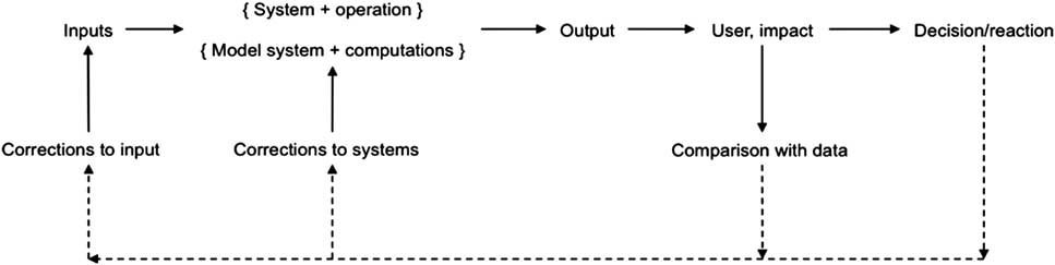
Figure 1 A schematic diagram showing action flow (solid) and information flow (dashed) in actual systems; and also information flow in model systems (which also lead to consequences for users and decision-makers).
Reductionist models are built up from sub-models and data of basic processes, such as scientifically established laws or processes (e.g. climate models). By contrast, empirical ‘statistical’ models are based on past data, which may be specific to the system, because there are no reliable models for the entities in the system (e.g. financial trading or certain types of seasonal forecasting). The disadvantage of purely statistical models is that they rely on past data and cannot reliably be used in situations where external conditions or the entities themselves are changing and evolving. This is the main justification for the use of largely reductionist models for predicting climate change rather than relying on the extrapolation of current trends. Mixed reductionist and statistical models are also common, such as those involving natural and social systems.
Broadly, systems and their models fall into one of five categories (see Table 1). The first, denoted by X 0, being non-complex, comprising defined entities and connections between them. There are simple relations between inputs and outputs, such as in electrical or mechanical systems. The behaviour is often linear but non-linearity is possible. Typically for these systems, resonance is the most influential behaviour. Models of X 0 systems can be applied to describe features of very complex systems. For example, RichardsonReference Sutherland7 proposed a linear set of differential equations to describe the complex features of an arms race between two nations.
Table 1 Categories of complex system behaviour

In the lowest category of systems that can be characterized as being complex – denoted by X 1 – there are typically a few types of well-defined sub-systems that have semi-spontaneous, self-organizing behaviour that depends only weakly on external influences and the previous states or history of the system. An example is the repetitive formation of cloud shapes, or patterns of vibrations of most mechanical systems.Reference Thompson and Bishop21X 1 systems respond to external conditions and inputs in a defined statistical sense, even if their behaviour cannot be predicted exactly. Decisions about risk in such systems have to allow for behaviour to occur unpredictably with very large amplitude, such as ‘rogue’ ocean waves, or sudden price movements (a focus of ‘complexity economists’Reference Bienhocker18).
The second category of complex system, X 2, are multi-type systems with generic differences in their component entities and sub-systems. X 2 systems have to be modelled using a range of sciences and technologies. The behaviour of such systems is less predictable a priori, because the different types of sub-system are open to different, and often unknown, influences. Nevertheless, observations and experience show that these multi-type systems can have patterns of behaviour that are common to other systems with comparable connectivity and interactions between entities (see section 3). There are large gradients over space and time and differing time scales of significant processes. Examples of X 2 systems include models of weather and climate; traffic flow; basic biological systems such as cells; and certain, well-defined, social units.
The third type of characteristic system, X 3, has a higher degree of complexity since the forms of the entities and connections are transformed into some new forms with persisting characteristic behaviour. In other words, such systems are interactive, adaptive and generally chaotic (IAC), since their behaviour depends sensitively on their previous behaviour as well as on input conditions and external influences. This category describes most living systems ranging from simple organismsReference Prigogine and Stengers12 to the entire Earth system.Reference Vernadsky22 Large organizations and governments fall into this category, as they adapt and evolve under external influences and varying inputs to the system. Models of X 3 systems have to account for uncertainty associated with unpredictable feedback from agents and other systems.
Note that some collections of interacting entities cannot be described as systems if their individual and group behaviours have no internal memory, if outputs are uncorrelated to inputs, and if the internal connections and properties of the entities keep changing (e.g. perfectly elastic spheres in a containerReference Hansen23).
As theory and observation show, there are limits to the accuracy of models, notably about prediction and about adaptation, which depend on the structure and nature of the system. Such errors naturally affect the reliability of decisions based on the models and need to be understood by decision-makers, as well as knowing whether such errors can be reduced, and at what cost.
With computers operating faster and accessing ever-greater volumes of data, and with greater capacity and speed of communication, it is technically possible to construct model systems that operate and control ever-larger artificial systems, such as networks of communications, computers or transportation. Similarly, it is possible, in principle, to compute formal models of partially continuous systems with ever-greater numbers of entities and types of sub-system.
Research and experience shows that in the operations of large real systems, sudden and unpredicted events can occur, or the systems can become unstable. For similar reasons, errors in the models can grow unexpectedly. Much research is directed at showing under what conditions such events occur and how, by comparing observations and model behaviour, and correcting the models through the technique of data assimilation, the accuracy, and also understanding, of the models can be greatly improved.
3. Decisions and Connectivity
3.1. Connectivity
Between the sub-systems and entities in complex systems there are connections that are local; for example, between adjacent eddies or organisms, and connections that are non-local and which extend over groups of entities within the system (such as between the atmosphere and ocean, or between groups of species). In systems with characteristic types of behaviour, the nature of these connections, and their complexity, largely determine the main features of behaviour and can explain the different patterns of behaviour in disparate systems. Focusing on connectivity helps understand modelling, designing and deciding about the underlying properties and the common features of real systems and their models – even the frustrating behaviour of transport systems during major disruptions. Connectivity is often the key to decisions taken by managers of organizations and by designers, repairers, and operators of conceptual and physical systems. Heart surgeons and architects have to be topologists as they deal with intersection points in arteries and buildings.Reference Hunt, Abell, Peterka and Woo24, Reference Steadman25
Following Euler, many aspects of connectivity can be described in terms of idealized networks and intersection points, which, like underground maps, are idealized depictions of reality. Typically, a system can be modelled as N distinct and labelled entities or nodes. The strength of the connection between the ith and the jth node is denoted by cij – which can vary between 0 and 1. Following Barrat et al. Reference Barrat, Barthelemy, Pastor-Satorras and Vespignani26,
networks are specified not only by their topology but also by the dynamics of information or traffic flow taking place on the structure. In particular, the heterogeneity in the intensity of connections may be very important in the understanding of social structure.
Graphs may represent one-way or two-way connections, up to a maximum of N(N−1). Thence, an overall measure of connectivity C can be defined as the average of cij,
so that C = 0 in a totally disconnected network and C approaches unity in networks with high connectivity. The local connectivity or ‘clustering’ of the interactions in a system can also be defined objectively in terms of the average value of cij for entities whose distance apart lij is small.
Complex systems, such as large physical systems or organizational systems, may have different connections and/or weightings for information and for action between the entities or nodes. Insight on the functioning of organizational networks can be gained by considering the connectivities in these networks, denoted by CI and CA respectively.
In hierarchical, strongly managed or secretive organizations, the connections may be strong (i.e. cij = 1 or is close to unity) but the number of connections across the organization may be deliberately small (so that CI and CA are of the order 1/N). On the other hand, in creative organizations there should be many connections – which may be relatively weak – to encourage ideas and originality (so that the average value of cij << 1 but C ≈ 1).
Managers of high-risk organizations realize the dangers of having too few connections when key elements of the organization or structure are damaged (see Section 3.2). Avoiding low connectivity between ecologically significant regions is also a critical objective of biodiversity policy.Reference Reza and Abdullah27 On the other hand, in social organizations, pathological behaviour of the whole organization can result from too many strong connections (with high values cij), as is sometimes seen in political groups and companies (where CI ≈ CA ≈ 1); for example, the scandal and system failure of EnronReference Healy and Palepu28 or information overload via the world wide web.
In buildings and structures, the connectivity of action between spaces, CA, varies between a small value (e.g. 1/N for a submarine) and a value close to 1 in the communal design of a typical ranch style or terrace house. Bentham's ideal of the Panopticon29 was for each room in the institution to be visible from a central atrium, but not inter-communicable, i.e. CA = 1/N. The three-dimensional geometry of how the actual spaces are connected is also of great importance for the functioning of buildings.Reference Steadman25 Resilient structures deliberately include some redundancy in their design, i.e. reduction in interconnectivity of actions CA, so that minor failures do not lead to major catastrophes.Reference England, Agarwal and Blockley30 But in some buildings CA is so large that they can collapse following the destruction of a limited part of the structure, as, for instance, the collapse of the Twin Towers in New York.31
Connectivity is also a useful concept for assessing models of complex systems, such as those for interconnected sub-systemsReference Greeves, Pope, Stratton and Martin32 of global climate change, seen in Figure 2. Here processes in one part of the system (e.g. oceans) are directly connected with a limited number of processes, and not directly connected with processes in other parts of the system (e.g. atmosphere-land) because of their different time scale and interfaces between them. The boundaries of the modelling systems have to be defined (as discussed in Section 3.3) – in Figure 2, the input assumptions and decision-making processes based on the global climate predictions are also assumed to be a part of the system. There are 14 (= N) modelling entities, and 32 connections between them, which is only a proportion of the total number of 182 (= N(N − 1)) possible connections, i.e. CA = 0.18, a quite low level of connectivity. This probably ensures a certain level of stability and lack of sensitivity to small changes in the models, but not to large changes, such as when Mitchell introduced aerosol effects.Reference Mitchell, Davis, Ingram and Senior33

Figure 2 The system of climate modelling and monitoring (both images reproduced with permission of the UK Meteorological Office). (a) Elements that have to be considered as variable, or fixed, parameters in weather or climate models depending on the timescale of the calculation (from days to millennia): the climate model has a small level of connectivity CA = 0.18. (b) Time scale of the development of more complex features of climate models, and the data sets used for verification such as those used by UK's MET Office Hadley Centre and the IPCC.
3.2. Breakdowns and Barriers
Design, operational and policy decisions about systems should be based on understanding how interactions between connections and entities behave in the event of possible disruptions. These have particular features where there are coupled networks in the system.
Consider a transport network with N entities, labelled from 1,2,…,N, which may be intersection points or stations (Figure 3). Suppose the matrix cij in Section 3.1 defines the connections between these entities. To estimate the effect of Nb breakages in the network (with just one breakage on each affected connection), it is assumed that the nodes at either end of the broken connections also cease operating. If each node has an average of ![]() connections (
connections (![]() for central London underground nodes), then the total number of connections affected, Nc say, is much greater than the number of breakages. In fact, for central London underground,
for central London underground nodes), then the total number of connections affected, Nc say, is much greater than the number of breakages. In fact, for central London underground,

Figure 3 Coupled train/underground and over-ground transport networks; note the inward flux of people by train FT and the diffusive fluxes FG in the over-ground system.
so that only a few simultaneous deliberate or accidental breakages can quickly affect a high proportion of the central part of a network. Angeloudis and FiskReference Angeloudis and Fisk34 confirmed how the three breakages in London on 7 July 2005, affected the whole central system (by affecting 30 connections according to equation (2) and, therefore, around 50% of the network).
However, infrastructure systems in cities are tightly coupled. The operation of the underground train network is closely linked to a much larger, more diffuse network, namely the ground transportation network, consisting of streets carrying vehicles and walkers. There are parallels with the movement of oil and water through porous rock and through connected cracks in the rock, or indeed with urban networks of fractured water mains.Reference Stuyt35
In a disrupted situation, modelling the concentration of people per unit area in the train system, PT(x,t), and on the ground, PG(x,t), at any time t and location x, can be greatly simplified by using a coupled diffusion process:
![\[--><$$>\eqalign{ \frac{{\partial {{P}_G}}}{{\partial t}}\, = \,{{S}_o}\, + \,{{S}_I}\,{\rm{ - }}\,k({{P}_G}\,{\rm{ - }}\,{{P}_T})\, + \,\nabla ({{D}_G}\nabla {{P}_G}) \\ \frac{{\partial {{P}_T}}}{{\partial t}}\, = \,k({{P}_G}\,{\rm{ - }}\,{{P}_T})\, + \,\nabla ({{D}_T}\nabla {{P}_T}) \\ \eqno<$$><!--\]](https://static.cambridge.org/binary/version/id/urn:cambridge.org:id:binary:20151126110613190-0606:S1062798711000585_eqnU5.gif?pub-status=live)
where SI is an influx of people into the central area and So is an outflow of people from the ground network into offices and building. DT and DG are the ‘diffusivities’ of the coupled networks. These equations describe the transition – from train to ground networks – when there is a breakdown in the train network. People transfer to ground transportation at a rate of the difference between PT(x,t) and PG(x,t).
The equations can approximate the flux (number of people per second per metre) of people on the train and ground networks, denoted by FT and FG respectively. In the outer parts of the city, these fluxes are proportional to the speeds of the train and the ground networks, bringing people into the centre. The fluxes are proportional to, and in opposite directions to, the spatial variation (or ‘gradient’) of the number of people per unit area, and the diffusivities of the networks. There are also fluxes FGT between the networks proportional to PT − PG.
The model shows how, when disruptions occur, travellers transfer from one network to the other. On the morning of the London terrorist attacks on 7 July 2005, when people were moving to the centre, a breakage in the train network meant DT decreased to zero in the centre, so that large concentrations of people rapidly developed near the disruptions and people surged onto the streets (i.e. PT and then FGT and PG increased). These tendencies were accentuated because of the lack of public information. Later the decision-takers controlled the situation by varying all these parameters through physical controls (e.g. road blocks reducing the value of DG) and provision of public communication, which led to people leaving the centre. Improved modelling of the physical and communications systems is essential to minimize risks in urban and other kinds of disaster.Reference White and Haas36, Reference Helbing37
Other types of geophysical hazards, whose importance depends on local circumstances, have to be predicted for many years into the future as urban areas grow in size and populationReference Hunt, Bohnenstengel, Belcher and Timoshkina38 and sea levels rise, raising the risks from tsunamis. In addition, one of the most serious hazards, which may interrupt telecommunications and electrical power for transport and environmental services, is the possibility of severe solar eruptions.
3.3. Systems with Boundaries
The structure and behaviour of most spatial systems and their models are greatly affected by how their boundaries form, move and perhaps break up in certain conditions. In most complex systems the external and internal boundaries are strongly related to the networks of connections joining entities within and on either side of boundaries. In these networks, agents or objects interact as they move between the various entities and spaces. For example, decision-makers have to identify and consider how to deal with internal boundaries that mark differences in functionality and levels of activity, for example disease or economic capacity (as in the ‘sure-start’ social improvement programmes in deprived urban areas in the UK and USReference Smith39, Reference Mujis, Harris, Chapman, Stoll and Russ40).
General models have been developed for the evolution and disruption of external and internal interfaces in systems with different properties or activities, such as those separating layers with different intensities of turbulence in the atmosphere. Modern research into active interfaces that occur within dynamic networks or continua shows that even though interactions between entities may occur, for example with agents moving between them, interfaces can remain sharp and do not necessarily smooth out as in simple diffusive processes. This is because there are counteracting processes, such as attractive forces and defensive instincts within social groups (or a physical system like stars and planets) much like the separation processes seen in Schelling's model of neighbourhood segregation.Reference Schelling41 Similarly, near the edges of crowds or turbulent flows, the people or eddies do not act like simple diffusive elements, because they cannot change direction fast enough (i.e. over a length scale that is short compared with the width of the flowReference Hunt, Eames and Westerweel42). Other examples are in blockages in flooding patternsReference Stelling and Tucker43 and brain networks.Reference Gray and Robinson13 Observers of the initial stages of riots in urban areas have noted how people stay within zones or move around community boundaries rather like fluid flow. To control these events, the connections and interactions between the zones are established, which also help deal with long-term consequences. However, civil and military decision-makers generally assume that with large enough disruptions near the interface or direct influences on local entities, interfaces can be disrupted. The cost of such a disruption is then of interest.
RichardsonReference Richardson44 first showed the power of applying these concepts to social systems in his analysis of the frequencies of conflicts between nations, which he found were correlated positively with the lengths L B of the boundaries B that separated them (recent geo-politics after 1989 seem to confirm this observationReference Sutherland7). Recent research on complex networks of biological systems, which have evolving interfaces that separate different parts of a network, is useful for models of diseased areas in a network, such as tumours.Reference Perfahl, Byrne, Chen, Estrella, Alarcon, Lapin, Gatenby, Gillies, Lloyd, Maini, Reuss and Owen45
4. System Changes and Decision-Making
4.1. Stability of the System
Decisions about a system involve first considering, for certain relevant external conditions, a number of possible future scenarios, which should be based on an understanding of the broad structure of the system and how it operates. Then decisions have to be made in the light of these possible scenarios. The scenarios can be represented schematically as graphs of the changes in the operation, or output, O(t), over time, t, depending on inputs or external influences (Figure 4(a)). In most realistic complex systems – natural, artificial or social – rapid changes occur at critical times, when the system might change to new kinds of persistent and robust scenarios (or ‘stable states’), or to other possible scenarios, which are not robust. A well-known example is how water heated in a saucepan is static until, at a certain level of heating, upward and downward eddy motions are generated (which have various stable forms). At this point the static scenario can no longer be stable.

Figure 4 Stability of system behaviour. (a) Diagram of stable (solid) and unstable (dashed) scenarios of a system; showing how its outputs O(t) or measure of decisions (e.g. carbon emissions associated with energy policy) vary with time t or amplitude of external disturbances A. Decisions follow a pathway of possible strategies following stable scenarios as they change with external interactions. (b) Dynamic system behaviour in relation to the speed of operation and speed of information processing/communication (such as traffic flow/decision making within an organization or an individual).
This kind of general analysis can lead to surprising predictions in new situations (such as Benjamin's analysis of types of swirling flow46). GladwellReference Gladwell47 describes examples of such ‘tipping points’. Some political scientists and historians have used these concepts to conclude that certain of types of rapid change of governmental structure are more stable than others, depending on the distribution of power and information between the top, middle and bottom of the organization – not unlike the heated water pan.
There is an ongoing debateReference Jaeger, Horn and Lux48 in most management, including governments, about how much to explain publicly (and for companies to explain to investors) the scenarios and their consequences that are under consideration. The advantage is that the public (or investors) can more easily understand and accept when decision-makers need to change policy and when new scenarios have to be considered following unforeseen events. Decision-makers are well aware that in complex systems, from weather to politics, the likely future states of the system are usually better predicted than the exact timing and the rapidity with which they will occur (although the latter information is what speculative investors really want).
With new methods of simulating complex organizations, for example by multi-agent models, and ever more comprehensive models of the scientific and technological aspects of the system, both the stable and unstable scenarios can be explored by decision-makers.
The system ‘map’ corresponds approximately to how some governments have been making decisions about energy and sustainability policies. The characteristic ‘states’ determine decisions about different energy sources (e.g. fossil/non fossil, etc.), all of which were feasible over the short term, say at time t 1, but as the consequences of these decisions become apparent for the long term (e.g. climate change and storage of nuclear wastes), and there is feedback from society, at time t 2 decisions in different countries change quite suddenly (e.g. to more non-fossil fuels, and relating energy decisions to those about sustainability). For example, the sharp changes seen in the UK and German government policy since 2003 including anti- and pro-nuclear policies were not driven by technical factors, but more by external political and social considerations.
An important question always is how, as decisions are made about future policies and explanations are given about future scenarios, organizations and individual agents respond and possibly adapt. Multiple consequences can be explored using simulations of the whole system. Agent-based modelling can simulate the effects on individuals and their feedback. Organizations may adapt by altering their external influences through interacting with the external systems that determine these influences, e.g. by plants forming their own ecosystems and by commercial advertising or political lobbying by organizations.
4.2. Dynamics of Change
Decision-makers need to know broadly how their particular system changes as a result of internal fluctuations or external influences. Often, decision-makers rely either on experience or intuition and incidental data. However, as some business and governmental decisions have demonstrated, dynamical systems concepts can provide both specific and general insights into how systems change with time naturally or deliberately, depending on their complexity and the data that are available in different conditions. This approach can indicate whether they are likely to change either smoothly or chaotically and intermittently, and whether the fluctuations are small or large. These tendencies affect how predictably the systems behave during these changes. Consequently, understanding these factors can assist making decisions about when to make decisions.
In well-defined systems with connected entities, changes can occur quite suddenly, even where change occurs repeatedly and with characteristic forms. Mathematical ‘catastrophe theory’Reference Saunders49 categorized the different types of sudden behaviour that can occur, whether abruptly, like a shock wave, or by growing fluctuations, or by a sudden transition into a different pattern, such as an ocean wave curling over and breaking. Applications to events in complex social systems have become possible as a result of many kinds of real-time observations and measurements of human activities and communications, which now are widely available in critical situations, such as dealing with hostages.Reference Zeeman50, 51
Where changes in a system build up with time (but not instantaneously) as a result of changing patterns of interactions between entities, they can be described and even predicted using general concepts, provided some basic data are available. The interactions may involve both physical and material actions on the one hand and information on the other, as they pass through the systems. A familiar example is a system of vehicles on roads driven by humans, with finite response times, influenced by real-time visual and electronic information. When the external influences change slowly and produce effects (e.g. slowing down of the traffic) over a longer time than the response time, each entity in the system can adjust smoothly. Typically, these ‘slow-local’ changes initially affect only some entities in the system before they have wider effects.
‘Slow-local’ changes in a system differ qualitatively from ‘fast-global’ changes that occur suddenly and either much faster than the response or predictability of the system or much faster than the speed at which entities interact. They may affect large parts of the system almost simultaneously, such as rapid natural disasters or stock market crashes. However, as science, technology and practice develop, with ever-faster data gathering and transmission speed, such rapid changes become redefined as ‘dynamic’ changes, as with disaster warning and some financial systems. In ‘slow-local’ systems, the throughputs of action or objects averaged over some characteristic region of the system, denoted by Q (units per second), are made up of ‘movements’ or fluxes of quantities (objects, activity, credit, ideas, etc) travelling through the system at an average speed V which varies markedly with the conditions in the system (Figure 4(b)). The throughput Q and speed V may vary through the system as entities are influenced by the speed c – at which information and action is transmitted through the system via the entities or agents within that system. Where Q varies, V also varies, leading to queues or accumulation of people, traffic, information, etc.
Changes in fluid flows, such as rivers, provide a good example to show how similar behaviour occurs in different liquid and gaseous systems. These concepts have already been used to analyse and control non-fluid systems.Reference Lighthill and Whitham52 In these flows, signal waves move with speed c through the fluid. In general, this differs from the speed of the flow V, which may be affected by the flow where it originates.
Where the flow has a speed V that is less than c, it responds immediately to speed changes elsewhere in the system (e.g. further along a river). This situation is not sensitive to local disturbances and is highly predictable. However when the ratio V/c (the Froude number for liquids or Mach number for gases) exceeds 1, the flow is faster than the speed of the waves or signals from elsewhere and cannot respond to distant signals (e.g. what happens downstream). Hydraulic engineers know – like managers experiencing a lack of timely data – that in this super-critical situation the system responds to extraneous influences in quite a different way to behaviour in sub-critical systems. In super-critical flow, the information is not transmitted fast enough to prevent ‘shocks’ where the throughput Q and the velocity are locally disturbed. In such cases, the position or timing of the sudden jump is very sensitive to disturbance and is often unpredictable.
A well-known example of similar behaviour in a non-fluid system is the variation in the moving patterns of traffic density or ‘stop-start waves’ on highways, which approximately correspond to the compressible flows of gases.Reference Lighthill and Whitham52 As usual, however, similarities have to be considered carefully. Traffic has two forms of flow depending on the same ‘Mach’ ratio of speed of cars, V, to speed at which ‘waves’ travel, c. The speed of waves, c, depends on the density of traffic and driver reaction time (typically c is about 40 km/h in near static conditions). As is well known, there is a slow flow where V/c < 1 and free flowing supercritical traffic where V/c > 1. The latter is an unstable situation – any blockage can soon lead to a ‘shock’ in the density and speed V of the vehicles. To predict in detail the behaviour of these systems with many agents requires computational simulations based on thousands of individual vehicle movements, but a simple wave equation analysis is useful for strategic decisions. The system dynamics is affected by the effective information ‘speed’ c at which agents receive and respond to ‘signals’ (e.g. days to travel from one office in an organization to another or seconds to respond over a car's pausing in traffic).
The patterns of mass movements of people in streets and buildings have many of the same smooth/shock transitions. Systems modelling could be more widely used to avoid overcrowding events.51 There are many operational and social systems where the variation of throughput, Q, has similar characteristic variations depending on the relation between the speed at which the system operates (V) and the speed (c) with which information is considered or at which changes to the system propagates through it. Decision-makers might find this concept useful firstly for considering how organizations work and how they can be more effectively managed (e.g. by changing their characteristic parameters) and secondly for considering how to respond to situations, analogous to roadblocks on roads. Perhaps the answer is that the most effective organizations should operate near the critical value of V/c = 1. But if low risk is required then V/c should be less than 1. Applying this system dynamics approach to organizations, by detailed study with quantification of relevant parameters (V, c, etc) might help regulators and even shareholders assess companies in future.
These ideas are also guiding research into how individuals operate in the modern world where a certain imposed ‘speed’ V is required to deal with their activities (which they can choose to some extent). People's effectiveness, and perhaps even their happiness, are possibly determined by how this (partly self-imposed) speed V relates to an individual's innate speed c of processing information and responding to external influences. Perhaps the greatest contentment and physiological healthReference Holmes20 comes from operating close to the critical ratio, although LayardReference Layard53 implies that happiness comes with less risk, which corresponds to operating with V/c < 1.
This example shows how ‘systems-thinking’ can not only provide a scientifically based framework for decision-making, but also provide revealing concepts that can be communicated in layman's languages, worldwide.
Acknowledgements
We acknowledge the financial support of the Future and Emerging Technologies (FET) programme within the Seventh Framework Programme for Research of the European Commission, under the FET-Open grant agreement GSDP, number 266723. The authors are grateful for many conversations from colleagues in this project. JCRH is also grateful for support from NSF grant 0934592.
Julian Hunt is Emeritus Professor of Climate Modelling in the Department of Earth Sciences and Honorary Professor of Mathematics at University College London. He is a fellow of Trinity College, Cambridge and a visiting professor at the Delft University of Technology and Arizona State University. He is a Fellow of the Royal Society, a member of the UK House of Lords and a former director-general of the UK Meteorological Office. He is a member of the Academia Europaea.
Yulia Timoshkina is an Honorary Research Fellow in the Department of Mathematics at University College London. She is also responsible for developing Clean Energy projects for Gazprom Marketing and Trading. Her previous roles include Policy Advisor for the UK Department of Energy and Climate Change, working on the Smart Metering and Green Deal programmes. Before that she led research projects on climate change strategies and natural resources management at the Centre for Energy Studies of the University of Cambridge. Yulia was born in Uzbekistan, and grew up there before going to study for a degree in Engineering in Moscow from 1997 to 2002. Then she completed her master's and doctorate research within the Engineering department of the University of Cambridge between 2003 and 2008.
Peter Baudains is a researcher at University College London, working across the Department of Mathematics, Department of Security and Crime Science and the Centre for Advanced Spatial Analysis. His research interests are in the development of models and tools for the analysis of complex systems, with applications to global security, conflict and terrorism.
Steven Bishop is Professor of Non-linear Dynamics at University College London. His research interests include complexity science, chaos, bifurcations and phase transitions. He is interested in the application of models to inform policy-makers, a subject of the European coordinated action projects on global system dynamics and policy: GSD (www.globalsystemdynamics.eu) and GSDP (www.gsdp.eu). He is also the coordinator of a new European initiative, FuturICT (www.futurict.eu), which intends to unify the best scientists in Europe to explore social life on earth and everything it relates to.


