2 Main results

In this section, it is identified that the basic system (1.1) for the pandemic modelling possesses a very reach Lie symmetry depending on the parameters $a, \ \gamma, \ d_1$ and $d_2$ and the function k(t). First of all, we note that for the LSC, we need only the restrictions $d_1^2+d_2^2\neq0$ (otherwise, the system in question degenerates into the ODE system, which was solved in [Reference Cherniha and Davydovych11]), $k\neq0$ (otherwise, the system in question seems to be useless for applications) and $b\neq0$ and $\gamma\neq0,-1$ (otherwise, the system in question is linear, hence is also integrable).

First of all, we present a statement about the group of ETs of system (1.1). For this purpose, we apply the technique, which was developed in [Reference Akhatov, Gazizov and Ibragimov3, Reference Ibragimov, Torrisi and Valenti21] (see also Section 2.3 in [Reference Cherniha, Serov and Pliukhin14]).

Theorem 2.1 The group of the continuous ETs’ transforming system (1.1) to that with the same structure, that is,

(2.1) \begin{equation}\begin{array}{l} \overline{u}_{\overline{t}} = \overline{d_1} \Delta \overline{u}+\overline{u}(\overline{a}- \overline{b}\overline{u}^{\overline{\gamma}}), \\[2pt] \overline{v}_{\overline{t}} = \overline{d_2}\Delta \overline{u} +\overline{k}(\overline{t})\overline{u},\end{array}\end{equation}

is the infinite parameter Lie group generated by the transformations:

\begin{align*} \overline{t} &=\beta_1t+\alpha_0, \nonumber\\[2pt] \overline{x} &=\beta_2\left(x\cos \beta_0 +y\sin \beta_0\right)+\alpha_1, \nonumber\end{align*}

(2.2) \begin{align}\nonumber\\[-35pt]\overline{y}&=\beta_2\left(y\cos \beta_0 -x\sin \beta_0\right)+\alpha_2, \nonumber\\[2pt] \overline{u}&=\beta_3u, \ \overline{v}=\beta_4v+f(x,y), \nonumber\\[2pt] \overline{k}&=\frac{\beta_4}{\beta_1\beta_3}\,k, \ \overline{d_1}=\frac{\beta^2_2}{\beta_1}\,d_1, \ \overline{d_2}=\frac{\beta^2_2\beta_4}{\beta_1\beta_3}\,d_2, \ \overline{a}=\frac{a}{\beta_1}, \ \overline{b}=\frac{b}{\beta_1\beta_3^\gamma}, \ \overline{\gamma}=\gamma. \end{align}

Here, $\alpha_i\ (i=0,1,2)$ and $\beta_j \ (j=0,\dots,4)$ are the real group parameters with the restrictions $\beta_1\beta_2\beta_4\neq0, \ \beta_3>0,$ and f(x,y) is an arbitrary smooth function.

Sketch of Proof of Theorem 2.1 is based on the known technique for constructing the group of ETs. It is nothing else but a modification of the classical Lie method. In the case of system (1.1), one should start from the infinitesimal operator:

(2.3) \begin{align}E&=\xi^0(t,x,y,u,v)\partial_t+\xi^1(t,x,y,u,v)\partial_x+\xi^2(t,x,y,u,v)\partial_y+\eta^1(t, x,y,u,v)\partial_u\nonumber\\[3pt] &\quad +\eta^2(t, x,y,u,v)\partial_v+\zeta(t,x,y,u,v,k)\partial_k+\mu^1\partial_{d_1}+\mu^2\partial_{d_2}+\mu^3\partial_{a}+\mu^4\partial_{b}+\mu^5\partial_{\gamma}, \end{align}

being $\xi^0, \ \xi^1, \ \xi^2, \ \eta^1,\ \eta^2 \ $ and $\zeta$ to-be-determined functions, while $\mu^i \ (i=1,\dots,5)$ to-be-determined constants. The operator E involves the additional terms with the coefficients $\mu^i$ and $\zeta$ , because $d_1, \ d_2, \ a, \ b, \ \gamma$ and k(t) should be treated as new variables.

In order to find the operator E, we should apply Lie’s invariance criteria to the system of equations consisting of (1.1) and a set of differential consequences of k(t) w.r.t. the variables t, x, y, u and v. Of course, each consequence is equal to zero, excepting $\frac{\partial k}{\partial t}=k'(t)$ (the latter is not useful because it is identity). As a result, we obtain a multicomponent system consisting of equations from (1.1) and primitive equations like $\frac{\partial k}{\partial x}= 0$ . Applying to this system the Lie’s invariance criteria, that is, the second prolongation of the infinitesimal operator E, for deriving the system of determining equations, the coefficients $\xi^{0},\ \xi^{1},\ \xi^{2},\ \eta^1, \eta^2, \ \zeta$ and $\mu^i \ (i=1,\dots,5)$ were found. They have the form:

(2.4) \begin{equation}\begin{array}{l}\xi^0=C_1t+C_2, \ \xi^1=C_3x+C_4y+C_5, \\[3pt]\xi^2=C_3y-C_4x+C_6, \\[3pt]\eta^1=C_7u, \ \eta^2=C_8v+h(x,y),\ \zeta=\left(C_8-C_1-C_7\right)k, \ \mu^1=\left(2C_3-C_1\right)d_1, \\[3pt] \mu^2=\left(2C_3-C_1+C_8-C_7\right)d_2,\\[3pt] \mu^3=-C_1a,\ \mu^4=-\left(C_1+C_7\gamma\right)b,\ \mu^5=0,\end{array} \end{equation}

where $C_i, \ i=1,\dots,8$ are arbitrary constants and h(x,y) is an arbitrary smooth function. The operator (2.3) with the coefficients (2.4) generates the Lie group (2.2).

The sketch of the proof is now completed.

In order to provide a complete LSC of system (1.1), one should identify the principal algebra of invariance (see definition, for example, in [Reference Cherniha, Serov and Pliukhin14], page 23) from the very beginning. In fact, system (1.1) involves an arbitrary function k and several parameters (some of them can vanish). Thus, it should be considered as a class of systems of PDEs, if one is going to provide a rigorous LSC.

Theorem 2.2 The principal algebra of invariance of system (1.1) is infinite-dimensional Lie algebra generated by the operators:

(2.5) \begin{equation} \partial_x, \ \partial_y, \ y\,\partial_x-x\,\partial_y,\ F(x,y)\,\partial_v,\end{equation}

where F(x,y) is an arbitrary smooth function.

The proof of this statement can be derived in different two ways. The direct approach consists of application of the classical Lie method to the system (1.1), assuming that all parameters are arbitrary. The second way is useful if the group of ETs is known. So, having Theorem 1, we simply calculate when transformations (2.2) transform (1.1) in itself, that is, system (2.1) coincides with (1.1). The result immediately leads to formulae (2.5).

Now we present two main theorems, which completely solve the LSC problem for (1.1). It turns out that there are two essentially different cases, $d_1\neq0$ and $d_1=0$ , leading to absolutely different results.

Theorem 2.4 System (1.1) with $d_1=0$ (then automatically $d_2\neq0$ ) admits the extension of the principal algebra (2.5) only in four cases. In each case, the additional operators have the structure:

(2.6) \begin{align} X&=\xi^0(t,u)\,\partial_t+\xi^1(x,y)\,\partial_x+\xi^2(x,y)\,\partial_y+\eta^1(t,u)\,\partial_u\nonumber\\[3pt] &\quad +\left(G(t,x,y,u)+(\xi^0_t-2\xi^1_x+\eta^1_u)v\right)\partial_v,\end{align}

where the functions $\xi^1$ and $\xi^2$ form an arbitrary solution of the famous Cauchy–Riemann system:

(2.7) \begin{equation} \xi^1_x=\xi^2_y, \ \xi^1_y=-\xi^2_x, \end{equation}

and G is an arbitrary solution of the linear first-order PDE

(2.8) \begin{equation}G_t+u(a- bu^\gamma)G_u=k(t)\left(\eta^1+2u\xi^1_x-u\eta^1_{u}\right)+uk'(t)\xi^0+u^2k(t)\left(a- bu^\gamma\right)\xi^0_u.\end{equation}

In the operator X, the functions $\xi^0$ and $\eta^1$ depending on the parameters $\gamma$ and a have the forms :

1. (1) if $\gamma\neq1$ and $a\neq0$ then

   \begin{equation*}\xi^0=\alpha_1+\frac{\alpha_2e^{at}}{au}\left(a-a\gamma+b\gamma u^\gamma\right)\left(a-bu^\gamma\right)^{-1+\frac{1}{\gamma}}, \ \eta^1=\alpha_2e^{at}\left(a-bu^\gamma\right)^{\frac{1}{\gamma}};\end{equation*}

2. (2) if $\gamma\neq1$ and $a=0$ then

   \begin{equation*}\xi^0=\alpha_1-\gamma\alpha_2t, \ \eta^1=\alpha_2u;\end{equation*}

3. (3) if $\gamma=1$ and $a\neq0$ then

   \begin{eqnarray} \nonumber && \xi^0=\frac{a\,\omega^2F''(\omega)}{u(a-bu)}+\frac{2b\,\omega F'(\omega)}{a-bu}-\frac{2bF(\omega)}{a}, \\[3pt] \nonumber &&\eta^1=a\,\omega^2F''(\omega)+2bu\,\omega F'(\omega),\ \omega=\frac{a-bu}{u}\,e^{at};\end{eqnarray}

4. (4) if $\gamma=1$ and $a=0$ then

   \begin{eqnarray} \nonumber && \xi^0=\frac{F''(\omega)}{2bu^2}-\frac{F'(\omega)}{bu}+\frac{F(\omega)}{b}, \\[3pt] \nonumber &&\eta^1=-\frac{F''(\omega)}{2}+uF'(\omega),\ \omega=\frac{1}{u}-bt.\end{eqnarray}
   Here $\alpha_1$ and $\alpha_2$ are arbitrary parameters, while F is an arbitrary smooth function.

Proofs of Theorems 2.3 and 2.4 are based on the technique which is a combination of the classical Lie method and the group of ETs. This technique is often called the Lie–Ovsiannikov method because L.V. Ovsyannikov was the first person who applied such technique for solving the LSC problem (group classification problem) for a class of the non-linear heat equations [Reference Ovsiannikov30]. Here, we present the proof of Theorems 2.4 because that is more complicated compared with the proof of Theorem 2.3.

Proof of Theorem 2.4.

System (1.1) with $d_1=0, \ d_2\neq0$ can be rewritten as:

(2.9) \begin{equation}\begin{array}{l} u_t = u(a- bu^\gamma), \\[3pt] v_t = \Delta u +k(t)u.\end{array}\end{equation}

using an appropriate ET from (2.2). As usually, we start from the most general form of a Lie symmetry operator:

(2.10) \begin{equation} \begin{array}{l} X=\xi^0(t,x,y,u,v)\,\partial_t+\xi^1(t,x,y,u,v)\,\partial_x+\xi^2(t,x,y,u,v)\,\partial_y\\[3pt] \hskip1.5cm +\eta^1(t,x,y,u,v)\,\partial_u+\eta^2(t,x,y,u,v)\partial_v.\end{array}\end{equation}

In order to find all the Lie symmetry operators of the form (2.10) of system (2.9), one should apply the following invariance criterion :

(2.11) \begin{equation}\begin{array}{l}X_{1}\left(u_t - u(a- bu^\gamma)\right)\Big\vert_{{\mathcal{M}}} =0, \\[3pt] X_{2} \left(v_t-\Delta u -k(t)u\right)\Big\vert_{{\mathcal{M}}} =0,\end{array} \end{equation}

where operators $X_{1}$ and $X_{2}$ are the first and second prolongations of the operator X, and the manifold ${\mathcal{M}}$ is defined by the system of equations:

\begin{eqnarray} \nonumber && u_t = u(a- bu^\gamma), \ v_t = \Delta u +k(t)u, \\[3pt] && \nonumber u_{tt} = \left(a- b(\gamma+1)u^\gamma\right)u_t, \ u_{tx} = \left(a- b(\gamma+1)u^\gamma\right)u_x,\ u_{ty} = \left(a- b(\gamma+1)u^\gamma\right)u_y.\end{eqnarray}

It should be stressed that the manifold ${\mathcal{M}}$ involves not only the equations of the system in question but also the first-order consequences of the first equation of (2.9). These consequences guarantee a complete solving of the LSC problem. Notably, such peculiarity does not occur for scalar PDEs, but one was noted for some systems of PDEs involving equations of different order (see, e.g., the relevant discussion in [Reference Bluman, Cheviakov and Anco6] Section 1.2.5).

Having the correctly defined manifold ${\mathcal{M}}$ , the invariance criterion (2.11) after rather standard calculations leads to the system of determining equations as follows:

(2.12) \begin{eqnarray} && \xi^0_{x}=\xi^0_{y}=\xi^0_{v}=0, \ \xi^1_{t}=\xi^1_{u}=\xi^1_{v}=0, \ \xi^2_{t}=\xi^2_{u}=\xi^2_{v}=0, \end{eqnarray}

(2.13) \begin{eqnarray} && \eta^1_x=\eta^1_y=\eta^1_v=0, \ \eta^2_v=\xi^0_t-2\xi^1_x+\eta^1_u, \end{eqnarray}

(2.14) \begin{eqnarray} && \xi^1_x=\xi^2_y, \ \xi^1_y=-\xi^2_x, \end{eqnarray}

(2.15) \begin{eqnarray} &&\eta^1_{uu}=2\left(a-b\left(1+\gamma\right)u^\gamma\right)\xi^0_u+u\left(a- bu^\gamma\right)\xi^0_{uu},\end{eqnarray}

(2.16) \begin{eqnarray} &&\eta^1_{t}=\left(a-b\left(1+\gamma\right)u^\gamma\right)\,\eta^1+u^2\left(a- bu^\gamma\right)^2\xi^0_u+u\left(a- bu^\gamma\right)\left(\xi^0_t-\eta^1_{u}\right),\end{eqnarray}

(2.17) \begin{eqnarray} && \eta^2_t+u\left(a- bu^\gamma\right)\eta^2_u=k(t)\left(\eta^1+2u\xi^1_x-u\eta^1_{u}\right)\nonumber\\[3pt] && +uk'(t)\xi^0+u^2k(t)\left(a- bu^\gamma\right)\xi^0_u. \end{eqnarray}

Equations (2.12) and (2.13) can be easily integrated; hence, the general form of the infinitesimal operator (2.10) can be specified as (2.6). Now substituting the function:

\begin{equation*}\eta^2=G(t,x,y,u)+\left(\xi^0_t-2\xi^1_x+\eta^1_u\right)v,\end{equation*}

into equation (2.17) and splitting the equation obtained w.r.t. the variable v, we arrive at the linear equation (2.8) for G(t,x,y,u) and the equation:

(2.18) \begin{equation}u\left(a- bu^\gamma\right)\xi^0_{tu}+\xi^0_{tt}+u\left(a- bu^\gamma\right)\eta^1_{uu}+\eta^1_{tu}=0.\end{equation}

Obviously, equations (2.14) coincide with (2.7).

Thus, we need only to solve the overdetermined system of equations (2.15), (2.16) and (2.18) w.r.t. the functions $\xi^0$ and $\eta^1$ . This is a non-trivial task because the function $\xi^0$ depends on the dependent variable u in contrast to the standard situation for the systems of reaction–diffusion equations (see [Reference Cherniha, Davydovych and Muzyka12, Reference Cherniha and King13] and the papers cited therein). Differentiating equation (2.15) w.r.t. t, taking the second-order consequence of equation (2.16) w.r.t. u and making the relevant calculations, we were able to derive the simple relation:

(2.19) \begin{equation} \xi^0_{t}=\frac{\left(1-\gamma\right)\eta^1-u\eta^1_u}{u}.\end{equation}

Substituting the derivatives $\xi^0_{tu}$ and $\xi^0_{tt}$ derived from (2.19) into equation (2.18), one arrives at the classification equation:

\begin{equation*}(1-\gamma)\Big(u(a-bu^\gamma)\eta^1_{u}-u^2(a- bu^\gamma)^2\xi^0_u+(a\gamma-a+bu^\gamma)\eta^1\Big)=0.\end{equation*}

Thus, the following two cases must be examined separately : $\gamma\neq1$ and $\gamma=1.$

In the case $\gamma\neq1$ , one immediately obtains

(2.20) \begin{equation} \eta^1_{u}=u\left(a- bu^\gamma\right)\xi^0_u+\frac{\left(a-a\gamma-bu^\gamma\right)\eta^1}{u\left(a-bu^\gamma\right)}.\end{equation}

Differentiating equation (2.20) w.r.t. the variable u and substituting the expression obtained for $\eta^1_{uu}$ into equation (2.15), one arrives at the equation:

(2.21) \begin{equation} \xi^0_{u}=\frac{a\left(\gamma-1\right)\eta^1}{u^2\left(a-bu^\gamma\right)^2}.\end{equation}

Equations (2.20) and (2.21) can be easily integrated. The general solutions are

(2.22) \begin{equation}\xi^0=g(t)+\frac{f(t)}{au}\left(a-a\gamma+b\gamma u^\gamma\right)\left(a-bu^\gamma\right)^{-1+\frac{1}{\gamma}}, \ \eta^1=\left(a-bu^\gamma\right)^{\frac{1}{\gamma}}f(t),\end{equation}

if $a\neq0$ and

(2.23) \begin{equation}\xi^0=g(t), \ \eta^1=f(t)u, \end{equation}

if $a=0$ . Here, f(t) and g(t) are arbitrary smooth functions at the moment. In order to find the functions f(t) and g(t), one needs to substitute (2.22) and (2.23) into equation (2.16). As a result, cases ${(1)}$ and ${(2)}$ of Theorem 2.4 were identified.

In the case $\gamma=1$ , equations (2.15), (2.16) and (2.19) take the forms:

(2.24) \begin{equation}\begin{array}{l} \xi^0_t=-\eta^1_{u}, \\ \xi^0_{tu}+u(a- bu)\xi^0_{uu}+2(a-2bu)\xi^0_u=0,\\ \eta^1_{t}+2u(a- bu)\eta^1_{u}=(a-2bu)\,\eta^1+u^2(a-bu)^2\xi^0_u,\end{array}\end{equation}

while equation (2.18) is satisfied identically.

Now, one can isolate $\xi^0_u$ from the third equation of (2.24) :

(2.25) \begin{equation}\xi^0_u=\frac{\eta^1_{t}}{u^2(a-bu)^2}+\frac{2\eta^1_{u}}{u(a-bu)}+\frac{(2bu-a)\eta^1}{u^2(a-bu)^2}.\end{equation}

Substituting (2.25) into the second equation of (2.24) and the equation $\xi^0_{tu}+\eta^1_{uu}=0$ (i.e., the differential consequence of the first equation of (2.24) w.r.t. the variable u), we arrive at the equations:

(2.26) \begin{equation}\eta^1_{tu}+u(a-bu)\eta^1_{uu}+(a-2bu)\eta^1_u+2b\eta^1=0,\end{equation}

and

(2.27) \begin{equation}\eta^1_{tt}+2u(a-bu)\eta^1_{tu}+u^2(a-bu)^2\eta^1_{uu}+(2bu-a)\eta^1_t=0,\end{equation}

respectively.

It turns out that equation (2.27) is reduced to the ODEs w.r.t. the time variable:

\begin{equation*}\eta_{tt}+\left(a-\dfrac{2a\omega}{\omega+be^{at}}\right)\eta_{t}=0,\end{equation*}

and

\begin{equation*}(\omega+bt)\eta_{tt}+2b\,\eta_{t}=0,\end{equation*}

by the transformation:

\begin{equation*}\eta^1(t,u)=\eta(t,\omega), \ \omega=\left\{\begin{array}{l} \dfrac{a-bu}{u}\,e^{at}, \ a\neq0, \\ \dfrac{1}{u}-bt, \ a=0,\end{array} \right.\end{equation*}

in the cases $a\neq0$ and $a=0$ , respectively.

Integrating the above ODEs, we easily derive the general solution, that is, the function:

\begin{equation*}\eta^1=uH_1(\omega)+H_2(\omega), \ \omega=\left\{\begin{array}{l} \dfrac{a-bu}{u}\,e^{at}, \ a\neq0, \\ \dfrac{1}{u}-bt, \ a=0,\end{array} \right.\end{equation*}

where $H_1$ and $H_2$ are arbitrary smooth functions at the moment. Substituting the above function into (2.26), we arrive at the restriction:

\begin{equation*}H_2=\left\{\begin{array}{l} \dfrac{a}{2b}\left(\omega H_1'-H_1\right), \ a\neq0, \\ -\dfrac{H_1'}{2}, \ a=0.\end{array} \right.\end{equation*}

Thus, using notations $H_1=2b\omega F'$ (in the case $a\neq0$ ) and $H_1=F'$ (in the case $a=0$ ), one finds the function $\xi^0$ from the first equation of system (2.24)

\begin{equation*}\xi^0=\left\{\begin{array}{l}\dfrac{a\,\omega^2F''(\omega)}{u(a-bu)}+\dfrac{2b\,\omega F'(\omega)}{a-bu}-\dfrac{2bF(\omega)}{a}+g(u), \ a\neq0, \\ \dfrac{F''(\omega)}{2bu^2}-\dfrac{F'(\omega)}{bu}+\dfrac{F(\omega)}{b}+g(u), \ a=0,\end{array} \right.\end{equation*}

where g(u) is to-be-determined function.

Substituting the functions $\xi^0$ and $\eta^1$ into equation (2.25), we obtain $g(u)=const$ . As a result, cases ${(3)}$ and ${(4)}$ of Theorem 2.4 are derived.

At the final stage, the functions, $\xi^0$ and $\eta^1$ , should be inserted into (2.8). The equation obtained is an integrable first-order PDE and its general solution is easily constructed in an explicit form provided that the function k(t) is given. Thus, all the coefficients of operator (2.6) are identified.

The proof is now complete.

Let us present examples of highly non-trivial Lie symmetries in cases ${(3)}$ and ${(4)}$ (see Theorem 2.4). Setting $F(\omega)=\omega^3$ , one can specify the functions $\xi^0$ and $\eta^1$ as follows:

\begin{equation*} \xi^0=\frac{2}{au^{4}}\left(3a^2+2abu+b^2u^2\right)(a-bu)^2e^{3at}, \ \eta^1=\frac{6}{ u^{3}}(a+bu)(a-bu)^3e^{3at},\end{equation*}

and

\begin{equation*} \xi^0=\frac{1}{bu^3}-b^2t^3,\ \eta^1=3bt\left(btu-1\right),\end{equation*}

in cases ${(3)}$ and ${(4)}$ , respectively.

Now one should use the functions $\xi^0$ and $\eta^1$ for finding the function G from equation (2.8). In order to avoid cumbersome formulae, we additionally take the particular solution $\xi^1=y, \ \xi^2=-x$ of the Cauchy–Riemann system (2.7) and fix the function k(t) : $k(t)=e^{-3at}$ (case ${3)}$ ) and $k(t)=t^{-2}$ (case ${4)}$ ). As a result, one arrives at the Lie symmetry operators:

(2.28) \begin{align} X&= \frac{2}{au^{4}}\,\big(3a^2+2abu+b^2u^2\big)(a-bu)^2e^{3at}\partial_t+\frac{6}{ u^{3}}(a+bu)(a-bu)^3e^{3at}\partial_u \nonumber\\[3pt] &\quad +y\partial_x-x\partial_y +\Big(6b^3\ln u+\frac{3}{u^3}(a-bu)(2a^2-abu+b^2u^2)+H\left(x,y,\frac{a-bu}{u}\,e^{at}\right)\Big)\partial_v,\end{align}

and

(2.29) \begin{equation}\begin{array}{l} X=\left(\frac{1}{bu^3}-b^2t^3\right)\partial_t+y\partial_x-x\partial_y+3bt\left(btu-1\right)\partial_u\\[3pt]\qquad +\Big(-2b\ln (tu)+\frac{1-btu}{bt^2u^2}+H\left(x,y,\frac{1}{u}-bt\right)\Big)\partial_v\end{array},\end{equation}

in cases $\textit{(3)}$ and $\textit{(4)}$ , respectively. Here H is an arbitrary smooth function.

3 Exact solutions and their interpretation

Theorems 2.3 and 2.4 allow us to reduce the basic system (1.1) to that of lower dimensionality. In fact, using the Lie symmetry operators (or their linear combinations) listed in Theorems 2.3 and 2.4, one can reduce (1.1) to the corresponding $(1+1)$ -dimensional system and the latter to an ODE system. Here, we examine two cases in order to show that those lead to useful exact solutions.

First of all, one may simplify the non-linear system (1.1) using the ETs (2.2) with the correctly specified parameters:

\begin{eqnarray} \nonumber && \overline{t} =at,\ \overline{x}=\sqrt{\frac{a}{d_1}}\, x, \ \overline{y}=\sqrt{\frac{a}{d_1}}\, y,\\[3pt] \nonumber &&\overline{u}=\left(\frac{b}{a}\right)^{1/\gamma}u, \ \overline{v}=\left(\frac{b}{a}\right)^{1/\gamma}v,\end{eqnarray}

to the form:

(3.1) \begin{equation}\begin{array}{l} u_t = \Delta u+u(1- u^\gamma), \\[3pt] v_t = D \Delta u +\frac{1}{a}\,k\left(\frac{t}{a}\right)u, \ D=\frac{d_2}{d_1}. \end{array}\end{equation}

Here and in what follows, we preserve the old notations for all the variables.

Example 3.1. Let us apply the operator $\partial_y$ from the principal algebra (2.5) for reduction of the basic system (3.1). Obviously, this operator produces the trivial ansatz $u=u(t,x), \ v=v(t,x)$ , so that we arrive at the system:

(3.2) \begin{equation}\begin{array}{l} u_t = u_{xx}+u(1- u^\gamma), \\[3pt] v_t = D u_{xx} +\frac{1}{a}\,k\left(\frac{t}{a}\right)u, \ D=\frac{d_2}{d_1}. \end{array}\end{equation}

This system is nothing else but the initial system under the assumption that the distribution of the infected persons is one-dimensional in space (i.e., the diffusion w.r.t. the axis y is very small). In this case, the distribution of the total number of deaths will be also one-dimensional.

Making the further plausible assumption $d_1 \gg d_2$ , that is, the space diffusion of the infected persons leads mostly to increasing the total number of COVID-19 cases and not so much to new deaths, we may put $D=0$ . Following our previous paper [Reference Cherniha and Davydovych11], we specify the function $k(t)=k_0 e^{-\alpha t}$ (hereafter, $k_0>0, \ \alpha>0$ ). Thus, system (3.2) takes the form:

(3.3) \begin{equation}\begin{array}{l} u_t = u_{xx}+u\left(1- u^\gamma\right), \\[3pt] v_t = \frac{k_0}{a}\exp\left(-\frac{\alpha t}{a}\right)u. \end{array}\end{equation}

Using Theorem 2.3 (see case 4) therein), one notes that system (3.3) admits the Lie symmetry $\partial_t-\frac{\alpha }{a}\,v\partial_v$ . So, taking the linear combination of this operator and the operator $\partial_x$ :

\begin{equation*}X = c\partial_x + \partial_t-\frac{\alpha }{a}\,v\partial_v, \ c \in \mathbb{R},\end{equation*}

we obtain the ansatz:

(3.4) \begin{equation}u=\phi(\omega),\ v=\exp\left(-\frac{\alpha t}{a}\right)\psi(\omega), \ \omega=x-ct.\end{equation}

Substituting (3.4) into (3.3), one arrives at the ODE system:

(3.5) \begin{equation}\begin{array}{l} \phi''+ c\phi'+ \phi\left(1- \phi^\gamma\right)=0, \\[3pt] c\psi'+ \frac{\alpha}{a}\psi =-\frac{k_0}{a}\phi. \end{array}\end{equation}

The first equation in (3.5) is the known second-order ODE, which arises in many applications (e.g., for studying the Fisher equation and its natural generalisations [Reference Murray27]). The general solution of this ODE can be presented only in parametric form (see, e.g., [Reference Polyanin and Zaitsev32]), which is not useful for further analysis. However, an exact solution in the explicit form can be constructed for the correctly specified parameter $c=\frac{\gamma+4}{\sqrt{2(\gamma+2)}}$ . To the best of our knowledge, this parameter and the relevant solution were established in [Reference Abdelkader1] for the first time (see more references in [Reference Gilding and Kersner20]). As a result, we obtain the travelling front solution of the first equation in system (3.3):

(3.6) \begin{equation}u(t,x) =\left(1+ A\exp \left(\frac{\gamma}{\sqrt{2(\gamma+2)}}\,\omega\right)\right)^{-2/\gamma}, \ \omega=\pm\, x-\frac{\gamma+4}{\sqrt{2(\gamma+2)}}\,t, \ A>0.\end{equation}

Notably, (3.6) with $A<0$ is still a solution; however, one possesses a singularity. It should be also noted that the basic system (1.1) and its particular cases derived above are invariant under the discrete transformation $x \to -x$ ; therefore, we may put $\omega= x-\frac{\gamma+4}{\sqrt{2(\gamma+2)}}\,t$ in what follows.

Having the function u in the explicit form (3.6), one easily derives the function v from the second equation of system (3.3):

(3.7) \begin{equation}v(t,x) =\frac{k_0}{a}\int \exp\left(-\frac{\alpha t}{a}\right)\left(1+ A\exp \left(\frac{\gamma}{\sqrt{2(\gamma+2)}}\,\omega\right)\right)^{-2/\gamma}dt + g(x),\end{equation}

where g(x) is an arbitrary smooth function. The integral in the right-hand side of (3.7) cannot be expressed in the terms of elementary functions for arbitrary parameters $a, \ \alpha$ and $\gamma$ ; therefore, we study below a particular case.

In order to avoid cumbersome formulae, let us set $\gamma=1$ in system (3.3). In this case, the above exact solution takes the form:

(3.8) \begin{equation}\begin{array}{l} u(t,x) =\left(1+ A\exp \left(\frac{1}{\sqrt{6}}\,\omega\right)\right)^{-2}, \ \omega=x-\frac{5}{\sqrt{6}}\,t, \\v(t,x) =\frac{k_0}{a}\int \exp\left(-\frac{\alpha t}{a}\right)\left(1+ A\exp \left(\frac{1}{\sqrt{6}}\,\omega\right)\right)^{-2}dt + g(x).\end{array}\end{equation}

The integral in the right-hand side of (3.8) can be expressed in the terms of elementary functions for several values of the parameter $\frac{\alpha }{a}$ . Taking $\frac{\alpha }{a}=\frac{5}{6}$ , for example, we obtain

(3.9) \begin{equation}\begin{array}{l} u(t,x) =\left(1+ A\exp \left(\frac{1}{\sqrt{6}}\,\omega\right)\right)^{-2}, \ \omega=x-\frac{5}{\sqrt{6}}\,t, \\v(t,x) =g(x) -\frac{6k_0}{5a}\exp\left(-\frac{x}{\sqrt 6}\right)\left(A+ \exp \left(-\frac{1}{\sqrt{6}}\,\omega\right)\right)^{-1}.\end{array}\end{equation}

Now we turn to a possible interpretation of solution (3.9). First of all, the functions u and v should be non-negative for any $t>0$ and $x \in \mathbb{I}$ (here $\mathbb{I} \subset \mathbb{R}$ ) because they represent the densities. Obviously, the functions u is always positive. It is easily seen that each function g(x) satisfying the inequality:

\begin{equation*} g(x) \geq \frac{6k_0}{5a}\exp\left(-\frac{x}{\sqrt 6}\right)\left(1+ A\exp \left(-\frac{x}{\sqrt{6}}\right)\right)^{-1}, \end{equation*}

guarantees also non-negativity of v. In particular, one may take the function:

(3.10) \begin{equation} g(x) = \frac{6k_0}{5a}\exp\left(-\frac{x}{\sqrt 6}\right)\left(1+ A\exp \left(-\frac{x}{\sqrt{6}}\right)\right)^{-1},\end{equation}

which guarantees that the zero density of the deaths in the initial time $t=0$ , that is, $v(0,x)=0$ . The initial profile for the density of the COVID-19 cases is

\begin{equation*} u(0,x) =\left(1+ A\exp \left(\frac{x}{\sqrt{6}}\right)\right)^{-2}. \end{equation*}

Examining the space interval $\mathbb{I}=[x_1,x_2], \ x_1<x_2$ , we can calculate the total number of COVID-19 cases and deaths on this interval as follows:

(3.11) \begin{equation}\begin{array}{l} U(t)=\int_{x_1}^{x_2} u(t,x)dx, \\[3pt] V(t)=\int_{x_1}^{x_2} v(t,x)dx.\end{array}\end{equation}

So, substituting solution (3.9) into (3.11), we arrive at the formulae:

(3.12) \begin{equation}\begin{array}{l} U(t)=(x_2-x_1) - \sqrt{6}\Big[\Big(1+ A\exp \Big(\frac{x_1-\frac{5}{\sqrt{6}}\,t}{\sqrt{6}}\Big)\Big)^{-1}-\Big(1+ A\exp \Big(\frac{x_2-\frac{5}{\sqrt{6}}\,t}{\sqrt{6}}\Big)\Big)^{-1}\\[3pt]\hskip2cm +\ln\Big(1+ A\exp \Big(\frac{x_2-\frac{5}{\sqrt{6}}\,t}{\sqrt{6}}\Big)\Big)- \ln\Big(1+ A\exp \Big(\frac{x_1-\frac{5}{\sqrt{6}}\,t}{\sqrt{6}}\Big)\Big)\Big], \\[3pt] V(t)= \int_{x_1}^{x_2} g(x)dx - \frac{6\sqrt{6}\,k_0}{5a}e^{-\frac{5}{6}\,t}\Big[ \ln\Big(1+ A\exp \Big(\frac{\frac{5}{\sqrt{6}}\,t-x_1}{\sqrt{6}}\Big)\Big)-\ln\Big(1+ A\exp \Big(\frac{\frac{5}{\sqrt{6}}\,t-x_2}{\sqrt{6}}\Big)\Big].\end{array}\end{equation}

Obviously, the functions U(t) and V(t) are increasing and bounded, because

\begin{equation*} (U,V) \to \Big((x_2-x_1), \int_{x_1}^{x_2} g(x)dx \Big) \ as \ t \to +\infty. \end{equation*}

Moreover, taking the appropriate function g(x), we can guarantee that

\begin{equation*} U(0)=U_0\geq 0, \ V(0)=V_0\geq 0.\end{equation*}

Thus, one may claim that the exact solution (3.9) possesses all necessary properties for the description of the distribution of the COVID-19 cases and the deaths from this virus in time-space (under 1D approximation).

Examples of the exact solution (3.9) with the specified parameters and the corresponding functions (3.12) are presented in Figures 1 and 2. Notably, the parameters a and $k_0$ were taken approximately the same as in [Reference Cherniha and Davydovych11]. It follows from Figure 1 that the spread of the COVID-19 cases in space has the form of a travelling wave and this coincides (at least qualitatively) with the real situation in many countries. In Ukraine, for example, the COVID-19 pandemic started in the western part and then spread to the central and eastern parts of Ukraine (the major exception was only the capital Kyiv, in which the total number of COVID-19 cases was high from the very beginning). The distribution of deaths in space has more complicated behaviour (see the right plot in Figure 1). On the other hand, it is easily seen from Figures 1 and 2 that $v(t,x)\ll u(t,x)$ what is in agreement with the measured data in many countries [5]. Notably, the behaviour of the function v(t,x) can be essentially changed by the appropriate choice of the function g(x).

Figure 1. Solution (3.9) and (3.10) of the nonlinear system (3.3) with $\gamma=1$ . The function u(t,x) (left surface) describes the density of the COVID-19 cases, while the function v(t,x) (right surface) describes the density of deaths. The parameters are $k_0=0.01$ , $a=0.3$ and $A=1$ .

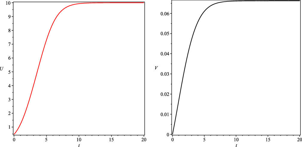
Figure 2. The functions (3.12) with (3.10). The function U(t) (left curve) shows the time evolution of the total number of COVID-19 cases on the space interval [0,Reference Cherniha and Davydovych10], while the function V(t) (right curve) shows the time evolution of total deaths. The parameters $k_0, \ a$ and A are the same as in Figure 1.

Example 3.2. Let us apply the operator $y\partial_x-x\,\partial_y$ from the principal algebra (2.5) for the reduction of the basic system (3.1). Obviously, this operator produces the well-known ansatz $u=u(t,r)$ , $v=v(t,r)$ and $r^2=x^2+y^2$ , that is, we examine the radially symmetric case. In this case, we arrive at the system:

\begin{eqnarray} \nonumber && u_t = \frac{1}{r}\left(ru_{r}\right)_r+u\left(1- u^\gamma\right), \\ \nonumber &&v_t = D \frac{1}{r}\left(ru_{r}\right)_r +\frac{1}{a}\,k\left(\frac{t}{a}\right)u, \ D=\frac{d_2}{d_1}. \end{eqnarray}

Making the same assumptions $k(t)=k_0 e^{-\alpha t}$ and $d_1 \gg d_2$ , that is, $D=0$ , as in Example 3.1, we obtain the system:

(3.13) \begin{equation}\begin{array}{l} u_t = \frac{1}{r}\left(ru_{r}\right)_r+u\left(1- u^\gamma\right), \\v_t = \frac{k_0}{a}\exp\left(-\frac{\alpha t}{a}\right)u. \end{array}\end{equation}

We have proved that system (3.13) again admits the Lie symmetry $\partial_t-\frac{\alpha }{a}v\partial_v$ (however, the operator of the space translation $\partial_r$ is absent in this case). So, using this symmetry, one obtains the ansatz:

(3.14) \begin{equation}u=\phi(r),\ v=\exp\left(-\frac{\alpha t}{a}\right)\psi(r), \ r=\sqrt{x^2+y^2}.\end{equation}

Substituting (3.14) into (3.13), one arrives at the system:

\begin{eqnarray} \nonumber && \phi''+ \frac{1}{r}\phi'+ \phi(1- \phi^\gamma)=0, \\[3pt] \nonumber &&- \frac{\alpha}{a}\psi =\frac{k_0}{a}\phi. \end{eqnarray}

Now one realises that the restriction $\alpha<0$ should take place because the function v means the density. So, the density of deaths increases to infinity as $t \to \infty$ . It means that the exponential growing of the function v is rather unrealistic because one obtains the total extinction of the population in question for a finite time. Thus, one should solve numerically the non-linear system (3.13) in order to get a realistic solution. Notably, numerical solutions of the Fisher-type equation from (3.13) can be found, for example, in [Reference Jordan and Puri22].