


INTRODUCTION
There is a growing consensus among scientists and the general public that the climate is changing, and that this trend is likely to have serious impacts not only on natural ecosystems, but also on human well-being (IPCC [Intergovernmental Panel on Climate Change] 2007a, b; EEA [European Environment Agency] 2004; Reid et al. Reference Reid, Mooney, Cropper, Capistrano, Carpenter, Chopra, Dasgupta, Dietz, Duraiappah, Hassan, Kasperson, Leemans, May, McMichael, Pingali, Samper, Scholes, Watson, Zakri, Shidong, Ash, Bennett, Kumar, Lee, Raudsepp-Hearne, Simons, Thonell and Zurek2005). Over the past 100 years, the mean global surface temperature has risen by about 0.7°C, exceeding the natural variation over the past 1000 years (IPCC 2007a). Evidence of climate change impacts are also accumulating, as evinced by reductions in the size of glaciers, upward shifts in tree lines and increases in the length of the growing season (IPCC 2007b). Furthermore, phenological changes and range shifts have been observed in many taxa (IPCC 2007b).
Anticipating future trends in climate can help governments adapt to potential impacts and implement relevant policy measures. The IPCC has developed a range of alternative emissions scenarios, based on different socioeconomic development pathways for the 21st century (Nakicenovic et al. Reference Nakicenovic, Alcamo, Davis, de Vries, Fenhann, Gaffin, Gregory, Grübler, Jung, Kram, Rovere, Michaelis, Mori, Morita, Pepper, Pitcher, Price, Riahi, Roehrl, Rogner, Sankovski, Schlesinger, Shukla, Smith, Swart, van Rooyen, Victor and Dadi2000). There is broad agreement between the general circulation models (GCMs), which were run for the emissions scenarios, that global mean global surface temperature is likely to rise between 2.0 and 4.5°C by the end of the century (IPCC 2007a). There is however considerable spatial variation in the projected changes. In addition, there is disagreement between the GCMs in relation to regional climate patterns and projected changes in precipitation (Ruosteenoja et al. Reference Ruosteenoja, Carter, Jylhä and Tuomenvirta2003). In order to account for this uncertainty, the IPCC recommends the usage of climate data from multiple GCMs in all climate change impact assessments.
Impact models applied to gridded spatial datasets, containing simulated climate variables for future time periods (for example see Hulme et al. Reference Hulme, Conway, Jones, Jiang, Barrow and Turney1995; Mitchell et al. Reference Mitchell, Carter, Jones, Hulme and New2004), have been used to further assess potential climate change impacts at global or continental scales. Examples are the global impact assessment model IMAGE (IMAGE Team 2001), the Lund Potsdam Jena dynamic global vegetation model LPJ-DGVM (Sitch et al. Reference Sitch, Smith, Prentice, Arneth, Bondeau, Cramer, Kaplan, Levis, Lucht, Sykes, Thonicke and Venevsky2003), and species distribution models (for example Thuiller et al. Reference Thuiller, Lavorel, Araújo, Sykes and Prentice2005). Because these modelling exercises generally cover large areas, involve many datasets and have to be performed for multiple scenarios and GCMs, the complexity of the interactions which can be incorporated is necessarily limited. Complex interactions are simplified, or approximated, and regional heterogeneity in pattern and process is ignored. In addition, these models require considerable technical expertise for their application. Nevertheless, analysis with such ecosystem models is very important for translating abstract changes in the climate variables into specific potential impacts that are more directly interpretable and relevant in both public debate and the policy arena.
This paper presents an alternative translation of a high-resolution gridded climate change dataset for Europe (Mitchell et al. Reference Mitchell, Carter, Jones, Hulme and New2004). Instead of determining climate response surfaces for specific species (Thuiller et al. Reference Thuiller, Lavorel, Araújo, Sykes and Prentice2005), biomes (IMAGE Team 2001), plant functional types (Sitch et al. Reference Sitch, Smith, Prentice, Arneth, Bondeau, Cramer, Kaplan, Levis, Lucht, Sykes, Thonicke and Venevsky2003) or forest growth (Sabaté et al. Reference Sabaté, Gracia and Sánchez2002), we determined climate functions for the 84 strata of the Environmental Stratification of Europe (EnS) (Metzger et al. Reference Metzger and Schröter2005a). The EnS was constructed by statistical clustering of mainly climate environmental variables into relatively homogeneous regions (for example distinct regions such as the British uplands, the Hungarian plains, the Po valley and numerous mountain regions, as well as statistically defined classes in regions with gradual environmental gradients). By fitting climate functions to the strata, a dataset has been constructed that illustrates how principal European environments are likely to shift under alternative climate change scenarios, in a similar way to earlier work on shifting biomes (see Tchebakova et al. Reference Tchebakova, Monserud, Leemans and Golovanov1993; Leemans et al. Reference Leemans, Cramer, van Minnen, Melillo and Breymeyer1996). However, the EnS distinguishes more classes than biome classifications (which only differentiate about eight classes in Europe), and it also partitions climate variation and the strata have strong correlations with wider environmental parameters across Europe, such as growing season, soil properties, species distributions (Metzger et al. Reference Metzger, Bunce, Jongman, Mücher and Watkins2005a) and habitats (Bunce et al. Reference Bunce, Metzger, Jongman, Brandt, De Blust, Elena-Rossello, Groom, Halada, Hofer, Howard, Kovar, Mücher, Padoa-Schioppa, Palinckx, Palo, Perez-Soba, Ramos, Roche, Skånes and Wrbka2008). The new dataset is therefore suitable for more detailed assessments at more regional scales, as we demonstrate for four sample regions.
While the EnS strata are generic compared to modelling exercises conducted for a specific issue (such as biodiversity, forestry and carbon sequestration), they provide a convenient summary of projected European climate shifts. Under current climate conditions, the EnS strata show significant correlations with a range of ecological factors. While these links may change in the future (Prentice et al. Reference Prentice, Cramer, Harrison, Leemans, Monserud and Solomon1992), the climate envelopes associated with the EnS strata provide useful units for determining potential changes in ecological resources (similar to ecological niche modelling; see Thuiller et al. Reference Thuiller, Lavorel, Araújo, Sykes and Prentice2005). The shifting strata have been applied to assess agricultural yield shifts under climate change (Ewert et al. Reference Ewert, Rounsevell, Reginster, Metzger and Leemans2005, Reference Ewert, Rounsevell, Reginster, Metzger, Leemans, Brouwer and McCarl2006) and vegetation change in a biodiversity assessment (Verboom et al. Reference Verboom, Alkemade, Klijn, Metzger and Reijnen2007). Furthermore, by combining the shifting strata with ancillary data, more complex analyses are possible, as demonstrated in this paper for four sample regions. In this way, the shifts in the distribution of strata can be used in the development of regional land-use change scenarios and to assess combined impacts of climate and land-use change on species dispersal (see del Barrio et al. Reference Del Barrio, Harrison, Berry, Butt, Sanjuan, Pearson and Dawson2006), as proposed by Opdam and Wascher (Reference Opdam and Wascher2004).
Because the EnS dataset of shifting environments is public, European environmental scientists have access to a convenient climate change dataset based on state-of-the-art emissions scenarios and multiple GCMs.
METHODS
We performed all GIS operations using ArcGIS version 8.2 (ESRI [Environmental Systems Research Incorporated] 2002) and statistical operations in SPSS version 11 (SPSS [Statistical Package for the Social Sciences] 2001) (Fig. 1).

Figure 1 Flow chart summarizing the development of the database of shifting European environmental strata and applications.
Datasets
Environmental stratification of Europe (EnS)
Stratification into relatively homogeneous regions is important for strategic random sampling of ecological resources, the selection of sites for representative studies across the continent and the provision of strata for modelling exercises (Metzger et al. Reference Metzger, Leemans and Schröter2005a). The EnS was created using tried-and-tested statistical procedures so that the strata are unambiguously determined and, as far as possible, independent of personal bias.
The EnS covers a ‘greater European window’ (11°W–32°E, 34°N–72°N), extending into northern Africa. This wider extent was needed to permit the statistical clustering to distinguish environments that have their main distribution outside the European continent. Furthermore, under future climate change, African environments are projected to expand into Europe (see Harrison et al. Reference Harrison, Berry, Butt and New2006), making it important to identify such environments.
Twenty of the most relevant available environmental variables were selected, based mainly on those identified by statistical screening (Bunce et al. Reference Bunce, Watkins and Gillespie1996c). These were (1) climate variables from the Climatic Research Unit (CRU) TS1.2 dataset (Mitchell et al. Reference Mitchell, Carter, Jones, Hulme and New2004), (2) elevation data from the United States Geological Survey HYDRO1k digital terrain model, and (3) indicators for oceanicity and northing. Data were analysed at 1-km2 resolution. Principal component analysis (PCA) was then used to compress 88% of the variation into three dimensions, which were subsequently clustered using an ISODATA clustering routine. The classification procedure is described in detail elsewhere (Metzger et al. 2005a).
The EnS consists of 84 strata, aggregated into 13 environmental zones (EnZs). These were constructed using arbitrary divisions of the mean first principal component score of the strata, with the exception of Mediterranean mountains, which were separated on altitude. Here we cover only 12 EnZs, as Anatolia (Turkey) is not covered in the current analysis. Within each EnZ, the EnS strata have been given systematic names based on a three-letter abbreviation of the EnZ to which the stratum belongs and an ordered number based on the mean first principal component score of the PCA. For example, the EnS stratum with the highest mean principal component score within the Mediterranean South EnZ is named MDS1 (Mediterranean South one). A detailed map of the EnS is provided as supplementary material to Metzger et al. (2005a).
Nine EnS strata occur in Africa, with four strata (MDS5–8) having their main distribution there. The most extreme stratum found in Europe (MDS7) was the hot and xeric environment around the Cabo de Gata in south-eastern Spain. MDS8 was restricted completely to the northern Sahara in Algeria and Tunisia.
Kappa analysis of aggregations of the strata shows they compare well with other European classifications (Metzger et al. 2005a, b). The EnS shows strong statistical correlations with other European environmental datasets (for example for soil and species distributions; Metzger et al. 2005a). The individual strata have been described using data from available environmental datasets.
High resolution grids of monthly climate
The TYN SC1.0 dataset consists of monthly climate information based on outputs from transient coupled atmosphere-ocean GCM simulations (Mitchell et al. Reference Mitchell, Carter, Jones, Hulme and New2004). The dataset has a spatial resolution of 10 arcmin longitude-latitude (for Europe approximately 16 km × 16 km), and contains mean monthly values for five climate variables from 2001–2100. A similar dataset of observed values (referred to as CRU TS1.2) covers 1901–2000 (New et al. Reference New, Lister, Hulme and Maken2002). The dataset variables are temperature, diurnal temperature range, precipitation, cloud cover and vapour pressure. We calculated four 30-year time slices for the climate datasets, as means of the variables, for the periods 1961–1990, 1991–2020, 2021–2050 and 2051–2080.
In order to provide as full a representation of the uncertainties in projections of regional climate change as possible, climate change scenarios were developed for four alternative greenhouse gas emissions scenarios and four GCMs. The emissions scenarios are based on the four narratives (A1, A2, B1 and B2) of the IPCC special report on emissions scenarios (SRES; Nakicenovic et al. Reference Nakicenovic, Alcamo, Davis, de Vries, Fenhann, Gaffin, Gregory, Grübler, Jung, Kram, Rovere, Michaelis, Mori, Morita, Pepper, Pitcher, Price, Riahi, Roehrl, Rogner, Sankovski, Schlesinger, Shukla, Smith, Swart, van Rooyen, Victor and Dadi2000). Each narrative is characterized by consistent driving forces of greenhouse gas emissions, including demographic change, economic development and technological development. To incorporate the range of potential changes that may occur for a given region and emissions scenario it has been recommended that the results from a number of GCM experiments are used (Viner Reference Viner2002). The four GCMs used in this study (discussed in detail in IPCC 2001) were HadCM3, CSIRO2, NCAR PCM and CGCM2. The 16 climate change scenarios resulting from the combination of the four GCMs and the four emissions scenarios cover 93% of the range of uncertainty for global warming in the 21st century published by the IPCC (Nakicenovic et al. Reference Nakicenovic, Alcamo, Davis, de Vries, Fenhann, Gaffin, Gregory, Grübler, Jung, Kram, Rovere, Michaelis, Mori, Morita, Pepper, Pitcher, Price, Riahi, Roehrl, Rogner, Sankovski, Schlesinger, Shukla, Smith, Swart, van Rooyen, Victor and Dadi2000).
Shifting environments
The original GIS file of the EnS (spatial resolution 1 km, equal area projection; Metzger et al. 2005a) was resampled to the 10 arcmin grid of the climate dataset (Mitchell et al. Reference Mitchell, Carter, Jones, Hulme and New2004), using the nearest neighbour resampling algorithm. Each grid cell of the 10 arcmin longitude-latitude EnS dataset was subsequently coupled to mean monthly values for the 1961–1990 average of four climate variables from the CRU TS1.2 dataset, namely temperature, diurnal temperature range, precipitation and cloud cover. Values for latitude and oceanicity (defined as the July–January temperature range divided by the sine of the latitude) were classification variables in the EnS and therefore also linked to each grid cell. By including latitude, differences in day-length and radiation were incorporated. Oceanicity expresses the buffering influence of the ocean, resulting in cooler summers, milder winters and a lower degree of interseasonal variability. The resulting attribute table consists of 31 143 rows (one for each grid cell), 48 climate attributes from the TYN SC1.0 dataset, latitude, the oceanicity index and an identifier for the EnS stratum to which each grid cell belongs.
SPSS was used to calculate Fisher's discriminant functions (Fisher Reference Fisher1936; McLachlan Reference McLachlan1992) for each EnS stratum. Given a set of interrelated variables, discriminant analysis determines linear combinations of those variables that best separate a set of distinct groups or classes. Fisher's linear discrimination rule finds a linear combination of the variables and determines the coefficients so that the ratio of the difference of the means of the linear combinations in the groups to its variance is maximized (Bunce et al. Reference Bunce, Watkins and Gillespie1996c).
The equality of group means was tested using one-way ANOVA for each variable in order to assess whether all 50 predictors (i.e. the monthly climate variables, latitude and oceanicity) could potentially contribute to the discriminant analysis. We also calculated Wilks’ lambda (a multivariate test statistic where lower values indicate that the variable is more effective at discriminating between groups) for each variable.
Fisher's linear discriminant functions were exported from SPSS and used in ArcGIS to determine the future distribution of the 84 strata from the monthly climate variables. Separate maps were created for the three time slices (2020, 2050 and 2080) for each emissions scenario and four GCMs (namely HadCM3, CSIRO2, NCAR PCM and CGCM2). The shift from the baseline environment was determined for the 2080 time slice in order to summarize the projected environmental shift for each grid cell. These shifts were summarised for each EnZ, indicating the direction of the shift, the area which had shifted to a different EnZ and the relative change in area of the EnZs. Student's t-test was used to analyse agreement in the shifts across GCMs and emissions scenarios.
The discriminant functions allocate an EnS stratum for each combination of climate conditions, effectively smoothing the original strata (Bunce et al. Reference Bunce, Watkins, Brignall, Orr and Jongman1996a). The 1969–1990 baseline strata of the EnS were compared with the strata allocation determined by the discriminant functions to test how accurately they reproduced the original classification. To test whether the shifted EnS strata did represent the climate change projected by the climate dataset, mean values of the climate variables were calculated for each EnS stratum under baseline conditions. For the future time slices, these values were used to project climate change as determined by the shifting EnS strata. For each EnZ, regional summaries of these projections were compared with regional summaries from the TYN SC1.0 climate dataset by linear regression through the origin and for seasonal averages of the climate variables. We also created box plots for the differences between the projected climate variables as expressed by the shifting EnS strata and the TYN SC1.0 dataset.
Sample regions
Whilst traditional modelling approaches (such as ecological niche modelling) provide specific information for a given entity (for example a species), the shifting strata provide more generic summaries of environmental shifts, which can be combined with ancillary data and expert knowledge to explore the potential impacts of climate change (Bunce et al. Reference Bunce, Watkins and Gillespie1996b). Such information supports the development of adaptation or conservation measures for environmental sectors or services important to the area, such as forestry, agriculture and the diversity and abundance of characteristic habitats and species. We selected four contrasting sample regions, namely southern Sweden, the southern Carpathian Mountains, the north-western Iberian Peninsula and south-western England and Wales (Fig. 2). We will primarily concentrate on the Swedish region, while the other regions illustrate contrasting impacts projected across Europe (see Supplementary material at http://www.ncl.ac.uk/icef/EC_Supplement.htm). The sample region in southern Sweden is mainly situated within the Nemoral EnZ, which includes Europe's northern limits for agriculture and deciduous tree species. Approximately 40% of the area is used as arable land, mainly for cereals (barley, oats, and wheat) as well as forage production (Eurostat NewCronos, URL http://epp.eurostat.ec.europa.eu). The remaining area is mostly covered by predominantly coniferous forest, with some beech (Fagus sylvatica) and oak (Quercus spp) forests in the south. Birch (Betula spp) is present throughout the region. Natural vegetation is determined by human induced agricultural and forest landscapes. Under the climate change scenarios, the region is projected to become warmer and wetter.

Figure 2 Map of Europe showing the location of the four sample regions. (A) southern Sweden, (B) the southern Carpathian Mountains, (C) the north-western Iberian Peninsula and (D) south-western England and Wales.
For the sample regions, we produced maps of the EnS strata for baseline conditions and the 2080 time slice, for one emissions scenario and two GCMs, and seasonal maps of change in mean maximum temperature (in °C) and mean precipitation (in % change) to assist in the interpretation of the shifting strata. For the Swedish region, we produced maps for four GCMs, in order to show how variability between GCM projections was translated into the EnS strata. Finally, for each sample region we produced maps, and for Sweden a table, used to interpret potential impacts (for example on nature conservation). We collected data on growing season and wheat productivity (Ewert et al. Reference Ewert, Rounsevell, Reginster, Metzger and Leemans2005), agricultural land use (Eurostat NewCronos, URL http://epp.eurostat.ec.europa.eu), and maps of the distribution of Fagus sylvatica and Quercus ilex s.l. (Köble & Seufert Reference Köble and Seufert2001), potential natural vegetation (Bohn et al. Reference Bohn, Gollub and Hettwer2000) and principal land cover types (Mücher et al. Reference Mücher, Champeaux, Steinnocher, Griguolo, Wester, Heunks, Winiwater, Kressler, Goutorbe, ten Brink, van Katwijk, Furberg, Perdigao and Nieuwenhuis2001).
In most regions of Europe, there is a strong coincidence between land use, climate, geomorphology, soil and market demand (Metzger et al. 2005a). Shifting climate strata and some basic ancillary information can be used as a first indication of the potential impacts of climate change. More detailed regional assessments can be developed by combining further ancillary datasets on geomorphology and soils, as well as socioeconomic scenarios describing alternative changes in demand (see Rounsevell et al. Reference Rounsevell, Reginster, Araújo, Carter, Dendoncker, Ewert, House, Kankaanpää, Leemans, Metzger, Schmit, Smith and Tuck2006).
RESULTS
Shifting European environments
One-way ANOVA was significant for all variables and Wilks’ lambda varied between the variables. The oceanicity indicator had the highest value (0.337), indicating the lowest discriminating power. The temperature variables and latitude had the lowest values (0.023–0.086). Values for precipitation (0.140–0.230) and cloud cover (0.047–0.174) were greater.
The discriminant functions allocated 75% of the grid cells to the same strata as the original dataset, resulting in minor differences to the published distribution patterns (Metzger et al. 2005a); the centre of gravity remained the same. Individual strata varied from 38% to 98%. In seven cases, < 50% of the grid cells were allocated correctly. Because the variation was continuous and divisions were arbitrary, misplaced grid cells occurred most frequently around the boundaries of strata, especially where environmental gradients occurred over large distances (for example in Central Europe). Misplaced grid cells were assigned to relatively similar EnS strata (with an adjacent EnS number, indicating a similar position on the first principal component; Metzger et al. 2005a; see Supplementary material at http://www.ncl.ac.uk/icef/EC_Supplement.htm, Table S1). The problematic strata often had a wide geographical spread, for example stratum CON2 covers foothills in the Alps, Central Europe and the Balkans, while MDM5 covers the southern foothills of the Pyrenees, the Massif Central and the Apennines.
The regression analysis was significant in all cases (four variables, four emissions scenarios, four GCMs; R2 > 0.95). Nevertheless, box plots for the difference between the variables projected by the shifting EnS and the climate dataset showed that, for most regions, temperature change projected by the GCMs was about 2°C greater than that predicted by the shifting EnS (Fig. 3). Precipitation and cloud cover predictions by the shifting EnS closely resembled the climate dataset (Fig. 3).

Figure 3 Box plots for each environmental zone, showing the difference between four climate variables, as projected by the TYN SC1.0 climate dataset and values associated with the EnS strata. Box plots depict the smallest observation, lower quantile, median, upper quantile and largest observation.
Time series maps showed how environments expanded, contracted, shifted or remain stable (Fig. 4), for example strata that had their main baseline distribution in northern-Africa shifted into Europe, for two time slices and two different GCMs (Fig. 5). Projected shifts between EnZs are summarized within the multivariate environmental space, determined by the first two principal components of the PCA used to construct the EnS (see Metzger et al. 2005a; Fig. 6). When the maps for the different GCMs and scenarios are seen as independent observations of the future environment of Europe, all changes in extent are significant, except for Alpine North and Atlantic North (Table 1).
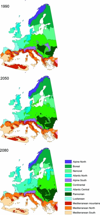
Figure 4 Shifting environmental zones in Europe assuming one climate change scenario (CGCM2 general circulation model; A2 emissions scenario) (Nakicenovic et al. Reference Nakicenovic, Alcamo, Davis, de Vries, Fenhann, Gaffin, Gregory, Grübler, Jung, Kram, Rovere, Michaelis, Mori, Morita, Pepper, Pitcher, Price, Riahi, Roehrl, Rogner, Sankovski, Schlesinger, Shukla, Smith, Swart, van Rooyen, Victor and Dadi2000; IPCC 2001).

Figure 5 Shifts in the four southernmost strata (MDS5–8, main distribution currently in northern-Africa) assuming the A1 emissions scenario (Nakicenovic et al. Reference Nakicenovic, Alcamo, Davis, de Vries, Fenhann, Gaffin, Gregory, Grübler, Jung, Kram, Rovere, Michaelis, Mori, Morita, Pepper, Pitcher, Price, Riahi, Roehrl, Rogner, Sankovski, Schlesinger, Shukla, Smith, Swart, van Rooyen, Victor and Dadi2000) and two general circulation models, namely the relatively modest NCAR PCM and the more extreme HadCM3 (IPCC 2001).

Figure 6 Shifting environmental zones, summarized across sixteen climate change scenarios, plotted in the environmental space of the classification variables of the environmental stratification of Europe. Arrows indicate the directions of projected shifts and the size of the shifting area (km2). Percentages refer to the change in extent of the environmental zones in 2080 compared to the 1990 baseline. Excepting ALN and ATN, changes are significant.
Table 1 Comparison to baseline conditions, summarized across sixteen climate change scenarios (four GCMs and four emissions scenarios). SE = standard error, 95% ll = lower limit, 95% ul = upper limit, T-test = Student's t-test, **significant at 1% level.

Southern environments shifted northwards (Fig. 6), confirming the concerns of the majority of climate change scientists. The drier and warmer Mediterranean South zone expanded northwards into the Mediterranean North environment indicating a potential expansion of desert habitats, and an increased risk of forest fires and drought. Lusitanian environments became drier and shifted into Mediterranean North, threatening endemic species and increasing the risk of droughts. Mediterranean Mountains and Alpine South environments decreased dramatically, becoming warmer Mediterranean North and Continental environments, respectively. Such a shift would have major implications for mountain plant species and ski tourism. The Continental zone underwent complex changes. In the centre it expanded into the Alpine and Carpathian mountain ranges. By contrast, in the east it shifted into the drier Pannonian, but in the west to the wetter Atlantic Central zone. Individual impacts are difficult to predict, but isolated habitats, such as low mountains and small nature reserves, are likely to change. Agriculture would also have to adapt to changing conditions. The Atlantic Central zone expanded northwards into Atlantic North, as well as into the Continental zone. Whilst the Atlantic environment is relatively stable compared to other regions, isolated habitats are likely to experience change. Agricultural productivity may increase under higher temperatures, although pests and diseases may also expand. In northern Europe, the GCMs made contradictory projections. As a result, changes for Atlantic North and Alpine North were not significant (Table 1; Fig. 4). Nevertheless there is agreement that Nemoral environments shift northward, and Boreal environments decrease in extent. Deciduous trees may be able to grow at more northern latitudes and higher altitudes. Forest structure could also significantly change. Permafrost will decrease in the north and associated habitats are highly threatened.
The sample region in southern Sweden
There was considerable variation in regional patterns between the four GCMs, especially for precipitation (Fig. 7). There was a general northward shift in the EnS strata. Changes in precipitation patterns will result in a strong expansion of Atlantic environments, which varied from a minor northwards shift of ATN5, the most northerly Atlantic stratum (HadCM3), to the arrival of Atlantic Central strata currently found in France (CGCM2). CSIRO2 projected a southward expansion of BOR8. This appeared to be caused by a strong increase in spring precipitation, characteristic of BOR8.

Figure 7 Shifting environments and climate change in the Swedish sample region and the current distribution of Fagus sylvatica (Köble & Seufert Reference Köble and Seufert2001).
The projected environmental shifts would have favourable consequences for plant growth, leading to an expanded growing season, higher temperature sums and higher productivity (Table 2). As a result, the region would become increasingly suitable for more temperate crops. More importantly, yields of currently grown crops are likely to increase significantly (Ewert et al. Reference Ewert, Rounsevell, Reginster, Metzger and Leemans2005). Similar increases in productivity would also occur for tree species, which would be favourable for forestry. Deciduous tree species (for example Fagus sylvatica, which has its northern limits in stratum NEM6; Fig. 7) could also expand northwards. While natural migration is likely to be slow, forest management could influence distribution patterns by creating spaces for regeneration. Climate change is also likely to influence biodiversity, for example through the expansion of weed species with southern distributions (such as Picris echioides). Nevertheless, management effects, both in agriculture and forestry, are likely to be more widespread than effects of climate change.
Table 2 Mean statistics for growing season, grain yield (Ewert et al. Reference Ewert, Rounsevell, Reginster, Metzger and Leemans2005), relative proportion of cereal crops (Eurostat NewCronos) and the relative area of two types of potential natural vegetation (Bohn et al. Reference Bohn, Gollub and Hettwer2000) for the ten strata projected to occur in the Swedish sample region (see Supplementary material at http://www.ncl.ac.uk/icef/EC_Supplement.htm for key to strata). – = no data available.

Examples of regional impacts in three other sample regions (the Carpathian mountains, the north-western Iberian Peninsula, and south-west England and Wales) are discussed online (see Supplementary material at http://www.ncl.ac.uk/icef/EC_Supplement.htm).
DISCUSSION
We aimed to construct an appropriate dataset for the analysis of shifting European environments under climate change. The utility of the final dataset depends on the definition of European environments and the quality of the climate change dataset. Both datasets used in this study were considered to be the most suitable of their kind at the present time.
The EnS forms the most detailed quantitative classification of the European environment currently available (Metzger et al. 2005a; Jongman et al. Reference Jongman, Bunce, Metzger, Mücher, Howard and Mateus2006). Despite the fact that climate variables were used to construct the EnS instead of bioclimate variables, the EnS strata show high correlations with both the annual temperature sum (R2 = 0.95) and the growing season (R2 = 0.83) (Metzger et al. 2005a), indicating that strata are strongly correlated with ecological parameters used in ecological niche modelling (see Thuiller et al. Reference Thuiller, Lavorel, Araújo, Sykes and Prentice2005). The choice of variables will have some influence on the class boundaries, but statistical environmental classifications will have much in common and decisions between them are arbitrary (Bunce et al. Reference Bunce, Carey, Elena-Rosello, Orr, Watkins and Fuller2002).
The TYN SC1.0 climate change dataset (Mitchell et al. Reference Mitchell, Carter, Jones, Hulme and New2004) has the highest spatial resolution of the gridded datasets available for Europe at this time and had been used in a range of state-of-the-art global change impact studies (for example Schröter et al. Reference Schröter, Cramer, Leemans, Prentice, Araújo, Arnell, Bondeau, Bugmann, Carter, Garcia, de la Vega-Leinert, Erhard, Ewert, Glendining, House, Kankaanpää, Klein, Lavorel, Lindner, Metzger, Meyer, Mitchell, Reginster, Rounsevell, Sabaté, Sitch, Smith, Smith, Smith, Sykes, Thonicke, Thuiller, Tuck, Zaehle and Zierl2005; Thuiller et al. Reference Thuiller, Lavorel, Araújo, Sykes and Prentice2005). A further advantage is that TYN SC1.0 data are available for four socioeconomic emissions scenarios and four GCMs, giving the maximum representation of uncertainties in regional climate change (see Fig. 7). Communication of the results from impacts assessments to the policy community is difficult and as yet there appears to be no suitable framework available to incorporate the sources of uncertainty, besides taking into account alternative development pathways and multiple GCMs (Viner Reference Viner2002).
The southern limit used in the present analysis, 34°N, was restricted by both the EnS and climate change dataset. Harrison et al. (Reference Harrison, Berry, Butt and New2006) used a coarser 0.5° climate dataset to train their ecological niche model for more southern climate conditions, using a southern limit of 15°N. Such an approach would be difficult to implement in the present methodology because it would entail constructing new environmental strata for the African domain. Despite the more modest southern limit, the results illustrate that even for the more extreme HadCM3-A1 scenario these African strata do not dominate the Iberian Peninsula (Fig. 5), suggesting that the EnS covers the climate conditions projected for Europe until 2080. The EnS acknowledges the environmental heterogeneity of the Mediterranean region, which is defined by 30 EnS strata (Fig. 5).
Discriminant analysis is an appropriate multivariate approach for assigning climate functions to previously determined strata (Bunce et al. Reference Bunce, Barr, Clarke, Howard and Lane1996b). Whilst the variation in Wilks’ lambda indicated differences in discrimating power between groups of variables (i.e. temperature being the most discriminating, followed by cloud cover and precipitation), the group means were significant for all variables, indicating that they also contribute to the function. Therefore, all variables were included in the discriminant analysis. Because misplaced grid cells occur mainly in strata which are relatively similar in climate properties, the implications for the interpretation of the results are limited.
One assumption in the current approach of shifting environments is that, while environments can shift, the relative climate profiles of the environments remain unchanged. The box plots (Fig. 3) show that this is not the case for temperature. In 2080, EnS strata are about 2°C warmer than under baseline conditions and the model is not sensitive to such small changes in temperature compared to more stable precipitation and cloud cover regimes. This is important in regions where environments do not shift, such as the British sample area (see Supplementary material at http://www.ncl.ac.uk/icef/EC_Supplement.htm). While at a European scale potential impacts in such regions are likely to be relatively minor, higher temperatures are significant at regional scales. For example, in Britain butterfly species have recently migrated northwards (Hill et al. Reference Hill, Thomas and Huntley1999) and larger numbers of migrating butterflies, including species considered as pests, are expected (Sparks et al. Reference Sparks, Roy and Dennis2005). A synthesis of UK research related to climate change and biodiversity conservation is available from www.ukcip.org.uk.
The analyses presented refer to environmental shifts, but are based on climate change scenarios only. As such, they could be misinterpreted. Whilst at a European scale environment is largely determined by climate (Metzger et al. 2005a), other important elements are independent, such as conurbations. Those that have a strong relationship with climate (for example potential natural vegetation and plant productivity) may be expected to change under projected shifts, but the independent elements are likely to be stable (for example many soils and urban structures). It is important to combine insights in climate shifts with ancillary information when assessing potential impacts for a specific region or issue. In the Swedish sample region (Fig. 7) there was a strong coincidence between land use and soil type. The acidic soils associated with the Scandinavian shield are dominated by forest cover, which limits the potential expansion of agriculture. Furthermore, agricultural expansion is unlikely when at a European scale agricultural land may be taken out of production, as suggested by alternative land-use change scenarios (Rounsevell et al. Reference Rounsevell, Reginster, Araújo, Carter, Dendoncker, Ewert, House, Kankaanpää, Leemans, Metzger, Schmit, Smith and Tuck2006). Regional soil conditions, land-use dynamics, competition and vegetation succession for colonizing deciduous species must all be considered; it is thus unlikely that deciduous tree species will be able to expand as rapidly as the shifting EnS strata indicate. The main conclusion for this sample region is therefore that climate change may exert a positive influence on agricultural and forestry production. However, from a European perspective, climate change is not likely to cause major shifts in land use or habitats in the region.
While the environmental shifts (Fig. 4) provided a condensed summary of projected shifts between EnZs, the 84 shifting EnS strata can be used as a statistical model to determine potential changes in ecological resources. EnS strata can be combined with agricultural statistics to make simple estimates of yield changes resulting from climate change (Ewert et al. Reference Ewert, Rounsevell, Reginster, Metzger and Leemans2005, Reference Ewert, Rounsevell, Reginster, Metzger, Leemans, Brouwer and McCarl2006). Similarly, the shifting strata have been used to determine changes in potential vegetation structure (Verboom et al. Reference Verboom, Alkemade, Klijn, Metzger and Reijnen2007). The dataset can also be used to assess changes in species distribution, especially for taxa at the edge of their range and where pools of more southern species are available for expansion. In this respect, islands such as Great Britain could be protected from rapid invasion of new species. While such models are less sophisticated than those constructed for one specific aim, they do provide clear information about projected climate shifts, including variability between climate change projections from multiple GCMs. When considerable uncertainty exists as to how the climate system will change, further investment in more complex modelling may not improve results.
Perhaps the most useful application of the shifting EnS strata is the option to combine insights into climate change with ancillary datasets and expert knowledge, thus linking landscape and biogeographical scales (Fig. 6; Supplementary material at http://www.ncl.ac.uk/icef/EC_Supplement.htm). In our examples, the ancillary data was limited to relatively few European datasets. When available, detailed regional datasets (for example for soil, species distribution and land use), field observations and local knowledge can be used to make more detailed assessments. Standard GIS operations can then be used to make regional scenarios, useful for evaluating regional or national physical planning and nature conservation. Such analyses can be extended to more complex modelling of meta-population behaviour and habitat change (Opdam & Wascher Reference Opdam and Wascher2004). Local effects of climate change on species distribution can be explored by integrating different models in a scale-dependant hierarchical framework, linking bioclimate niche models to land use and species dispersal models (Del Barrio et al. 2006). Similar approaches could be developed by linking shifting strata with dispersal models (Verboom et al. Reference Verboom, Alkemade, Klijn, Metzger and Reijnen2007). Such regional studies could be of interest to regional or national governments or non-governmental organizations (Del Barrio et al. 2006). Alternatively, by selecting representative sites across Europe, impacts on European habitats could be evaluated, or sample regions could be linked to socioeconomic scenarios describing different changes in demand (see Rounsevell et al. Reference Rounsevell, Reginster, Araújo, Carter, Dendoncker, Ewert, House, Kankaanpää, Leemans, Metzger, Schmit, Smith and Tuck2006). Consistent detailed global change scenarios could also be developed for selected regions across Europe.
CONCLUSIONS
The shifting EnS strata provide a convenient summary of the climate change scenarios. Monthly values for multiple parameters are summarized in classes with similar climate profiles. The results show that the dataset of shifting environmental strata conveniently summarizes contemporary knowledge about climate change in Europe. As such, it can be applied in simple modelling exercises, or in combination with ancillary data, to hypothesize potential change in ecological resources. The approach has the potential to facilitate a series of innovative approaches.
ACKNOWLEDGEMENTS
This work was carried out as part of the vulnerability assessment of the EU-funded Fifth Framework project ATEAM (Advanced Terrestrial Ecosystem Assessment and Modelling, Project No. EVK2-2000-00075). BSIK KvR project A-12 funded by Dutch Ministry for Agriculture, Nature and Food Security supported additional work. We especially thank the anonymous reviewers, whose constructive comments greatly improved the quality of the manuscript.


