


INTRODUCTION
The implementation of a mechanism for reducing carbon emissions from deforestation and forest degradation in developing countries (REDD) can constitute a competitive and cost-effective alternative to mitigate climate change and bring numerous benefits for environmental conservation (Kindermann et al. Reference Kindermann, Obersteiner and Sohngen2008; Ebeling & Yasué Reference Ebeling and Yasué2008; Venter et al. Reference Venter, Laurance, Iwamura, Wilson, Fuller and Possingham2009; Sangermano et al. Reference Sangermano, Toledano and Eastman2012). The estimation of reference emissions levels is one of the most challenging issues for REDD in developing countries (Verchot & Petkova Reference Verchot and Petkova2010; Scheyvens Reference Scheyvens2010; Sloan & Pelletier Reference Sloan and Pelletier2012). Reference emissions levels refer to the amount of emissions from deforestation against which any country's verified reduction will be credited (Busch et al. Reference Busch, Godoy, Turner and Harvey2011).
The United Nations Framework Convention on Climate Change (UNFCCC 2009) requests that countries should establish reference levels ‘transparently taking into account historic data, and adjust [them] for national circumstances’. This decision allows great flexibility on the approaches used for setting reference levels, which might be based on either historical or projected deforestation rates (Griscom et al. Reference Griscom, Shoch, Stanley, Cortez and Virgilio2009; Verbist et al. Reference Verbist, Vangoidsenhoven, Dewulf and Muys2011; Scheyvens Reference Scheyvens2010). Although reference emissions levels should consider historic data, decisions have not been made about the approaches countries should take to build reference levels (Verchot & Petkova Reference Verchot and Petkova2010; Cerbu et al. Reference Cerbu, Swallow and Thompson2011). The development of methods to integrate historic data with information about drivers of deforestation for building scenarios can improve the estimation of reference emissions levels and is a key research area for supporting the implementation of a REDD programme (Verchot & Petkova Reference Verchot and Petkova2010; GOFC-GOLD [Global Observation of Forest and Land Cover Dynamics] 2010; Corbera et al. Reference Corbera, Estrada and Brown2010; Alexandrov Reference Alexandrov2011).
The use of land change models to set reference emissions levels allows the incorporation of a variety of driving factors to predict deforestation, thus models can project scenarios of deforestation and carbon emissions based on possible changes of input variables as a consequence of changes in national circumstances and not just historic trends (Soares-Filho et al. Reference Soares-Filho, Nepstad, Curran, Cerqueira, Garcia, Ramos, Voll, McDonald, Lefebvre and Schlesinger2006; Parker & Mitchel Reference Parker and Mitchell2009; Umemiya et al. Reference Umemiya, Amano and Wilamart2010). This is particularly important for countries with historically low deforestation rates and a high proportion of forests remaining, which might be left out from any possibility of obtaining carbon credits if reference emissions levels are set based on only historic deforestation data (daFonseca et al. Reference da Fonseca, Rodriguez, Midgley, Busch, Hannah and Mittermeier2007; Cerbu et al. Reference Cerbu, Swallow and Thompson2011). Umemiya et al. (Reference Umemiya, Amano and Wilamart2010) found modelling land changes to be superior to using only historic data to develop REDD national reference levels since modelling can better reflect the national circumstances related to deforestation and the effect of policy efforts to reduce deforestation. Land change modelling has also proved useful in estimating REDD carbon benefits in project-level studies (Harris et al. Reference Harris, Petrova, Stolle and Brown2008; GOFC-GOLD 2010; Kim Reference Kim2010) and is recommended as best practice for the implementation of REDD projects by well-established international methodological standards (Estrada Reference Estrada2011).
Land change modelling has typically been used to predict future carbon emissions from deforestation by projecting how much and where deforestation will happen and then estimating emissions based on the carbon values assigned to the areas where deforestation is predicted (de Jong et al. Reference De Jong, Hellier, Castillo-Santiago and Tipper2005; Soares-Filho et al. Reference Soares-Filho, Nepstad, Curran, Cerqueira, Garcia, Ramos, Voll, McDonald, Lefebvre and Schlesinger2006; Brown et al. Reference Brown, Hall, Andrasko, Ruiz, Marzoli and Guerrero2007; Harris et al. Reference Harris, Petrova, Stolle and Brown2008). In these applications, land change modellers face the need to evaluate the accuracy of their models. Accuracy for land change models has been traditionally assessed based on the ability of a model to predict deforestation in terms of quantity (how much area will be deforested) and allocation (where deforestation will occur) (Pontius et al. Reference Pontius, Boersma, Castella, Clarke, de Nijs, Dietzel, Duan, Fotsing, Goldstein, Kok, Koomen, Lippitt, McConnell, Mohd Sood, Pijanowski, Pithadia, Sweeney, Trung, Veldkamp and Verburg2008a). However, if the purpose of using land change models is to estimate carbon emissions, then it makes more sense to evaluate a model based on its ability to estimate carbon emissions. This evaluation depends not only on the accuracy of the model to predict quantity and allocation of deforestation, but also on the information available about carbon, expressed similarly in terms of quantity (how much carbon is in the landscape) and allocation (how it is distributed in space) (Table 1).
Table 1 Components of uncertainty used to predict carbon emissions from deforestation.
In this paper, we analyse the influence of quantity and allocation of both carbon stocks and future deforestation on the prediction of carbon emissions from deforestation. For this purpose, we first introduce our conceptual framework by illustrating the analytical space where quantity and allocation come into play when predicting carbon emissions, and the degree to which the variation of each component influences the relative role of the others in the estimation of carbon emissions. Then we apply these concepts to a real case, based on published information about carbon mapping and deforestation modelling in the Brazilian Amazon. This paper does not intend to analyse all factors affecting uncertainty in the prediction of carbon emissions from deforestation. We argue that if the influence of factors can be quantified, then those factors can be expressed in the input carbon and land change maps as data ranges or predicted scenarios. Our method analyses available maps to express those data ranges or prediction scenarios in terms of quantity and allocation, and then evaluates their influence in the prediction of carbon emissions from deforestation. Our work, although potentially applicable, does not consider carbon removals or other REDD activities than deforestation.
Quantity and allocation of carbon and deforestation
To illustrate our conceptual framework, we assume that modellers have two maps. The first map shows the carbon density in every pixel in the study area at an initial year, typically expressed in Mg ha−1. The second map shows the pixels where deforestation is predicted cumulatively every year since the initial year of prediction. The information contained in both the carbon and the deforestation maps can be described in terms of quantity and allocation. From the carbon map, the sum of the carbon stocks in all pixels in the study area is the carbon quantity (CQ). Carbon allocation (CA) concerns the carbon density assigned to each pixel in the landscape. From the deforestation map, deforestation quantity (DQ) is the total cumulative proportion of the initial forest cover that a model predicts to be deforested at a specific year. Deforestation allocation (DA) refers to the spatial distribution of pixels where deforestation is predicted. Both CQ and DQ are non-spatial components of uncertainty since they can be represented numerically, regardless of how carbon or deforestation are distributed spatially. CA and DA are spatial components because they are best represented as a map.
To facilitate the description of our conceptual framework, we assume that once deforestation is predicted in a particular pixel, all carbon in that pixel is emitted. This is not the case in reality (Fearnside Reference Fearnside2000; Houghton Reference Houghton2005; Ramankutty et al. Reference Ramankutty, Gibbs, Achard, DeFries, Foley and Houghton2007). However, carbon emissions are usually predicted proportional or equal to the carbon density in pixels where deforestation is modelled (Soares-Filho et al. Reference Soares-Filho, Nepstad, Curran, Cerqueira, Garcia, Ramos, Voll, McDonald, Lefebvre and Schlesinger2006; Brown et al. Reference Brown, Hall, Andrasko, Ruiz, Marzoli and Guerrero2007; Castillo-Santiago et al. Reference Castillo-Santiago, Hellier, Tipper and De Jong2007; Harris et al. Reference Harris, Petrova, Stolle and Brown2008). Pontius et al. (Reference Pontius, Thontteh and Chen2008b) and Pontius and Millones (Reference Pontius and Millones2011) introduced the concepts of quantity and allocation, and demonstrated their value for comparing both continuous and categorical maps.
Carbon predicting space
The maximum amount of emissions that can be predicted for a given quantity of deforestation occurs when deforestation is allocated systematically in the pixels with the highest carbon values in the carbon map. Conversely, the minimum amount of emissions that can be predicted happens when deforestation is allocated in the pixels with the lowest carbon values. We refer to these two cases as the maximum and minimum emission scenarios (MaxE and MinE, respectively). The mean scenario (MeanE) corresponds to a case where carbon emissions are estimated as the mean carbon density in the study area multiplied by the total quantity of deforestation. Under the mean scenario, only information about quantity is considered. The mean scenario implicitly assumes a uniform distribution of carbon in the landscape, in which case MaxE and MinE would both be equal to MeanE.
Cumulative carbon emissions under the maximum, minimum and mean scenarios graphically resemble the shape of a leaf when deforestation quantity ranges from 0 to 100% (Fig. 1a). The upper and lower borders of the leaf represent the maximum and minimum emission scenarios for a given quantity of deforestation. The area bounded by these two scenarios is defined as the carbon predicting space, since any prediction of carbon emissions must fall on or between these two dashed boundaries. The central vein of the leaf is the mean scenario. The carbon map alone determines the predicting space, namely the edges and stem of the leaf. Larger spatial variation in the carbon map produces a wider leaf, while a more uniform spatial distribution produces a narrower leaf.

Figure 1 Components of uncertainty on the prediction of carbon emissions from deforestation. The horizontal axis is the quantity of cumulative deforestation (DQ) expressed as a percentage of initial forest cover. The vertical axis is the predicted carbon emissions expressed in units of mass of carbon. CQ is the total amount of carbon in the initial landscape represented by a particular carbon map. (a) Graphical representation of the maximum (MaxE), minimum (MinE), and mean (MeanE) scenarios and the carbon predicting space. (b) Influence of each component of carbon emissions. The influence of CQ (denoted by CQI) is measured as the total amount of carbon in the landscape and is independent of DQ. The influence of CA (denoted by CAI) is the difference between the maximum and minimum scenarios at a particular value of DQ. The influence of DQ (denoted by DQI) is measured as the carbon emissions under the mean scenario at a particular value of DQ. The influence of DA (denoted by DAI) is the modelled emissions minus the mean emissions at a particular value of DQ.
Influence of quantity and allocation of carbon and deforestation on predicted carbon emissions
We examine the relative influence of DQ, DA, CQ and CA on the prediction of carbon emissions and identify the maximum and minimum carbon emissions that can be predicted theoretically based on variations of these four components. We use the notation DQ, DA, CQ and DA to refer to concepts and we refer to their influence on carbon emissions by appending the letter I at the end of each two-letter abbreviation (for example DQI).
The influence of DQ on carbon emissions, DQI, corresponds to the estimation of carbon emissions using information about quantity only, namely the emissions calculated under the mean scenario for a particular value of DQ: DQI = DQ × CQ. This approach assumes that, in absence of spatial information about deforestation, carbon emissions are estimated by multiplying the total amount of deforestation by the mean carbon values in the study area, as has been suggested elsewhere (Gibbs et al. Reference Gibbs, Brown, Niles and Foley2007; Olander et al. Reference Olander, Gibbs, Steininger, Swenson and Murray2008). When quantity of deforestation is zero, emissions are zero. No other components of uncertainty influence the result since there is no deforestation to allocate. When quantity of deforestation is equal to 100%, then all the area is deforested, so carbon emissions depend uniquely on and are equal to the total quantity of carbon in the carbon map (CQ). At this extreme, allocation of carbon and deforestation are irrelevant because deforestation occurs in the entire area and the amount of predicted emissions is the same regardless of how carbon is allocated.
The influence of DA on carbon emissions, DAI, is visually represented by any curve that falls inside the carbon predicting space (Fig. 1b), where the curve is produced by a particular run of a model that predicts deforestation. DAI measures the effect of using spatial information about projected deforestation on predicting carbon emissions compared to not using spatial information at all, and therefore is measured as the emissions predicted by the modelled scenario minus the emissions represented by the mean scenario at any particular value of DQ (Fig. 1b). The magnitude of DAI depends on how the model allocates deforestation. If deforestation is allocated systematically in the pixels with the highest carbon values, then DAI is at its maximum possible value for a specific value of DQ and is positive. Similarly, if deforestation is allocated systematically in the pixels with the lowest carbon values, then DAI is at its minimum possible value for a specific value of DQ and is negative. If deforestation is allocated randomly, then carbon emissions will tend to be near the values obtained under the mean scenario, in which case DAI is near zero.
The influence of CQ on carbon emission, CQI, is represented in the leaf graph as the emissions when deforestation quantity is equal to 100% (Fig. 1b). Therefore CQI is measured as the total amount of carbon in the study area, thus CQI equals CQ. When CQ is zero, none of the other components of uncertainty matter in the estimation of carbon emissions. No carbon means that emissions are always zero, regardless of how much or where deforestation is predicted. As quantity of carbon is higher, the slope of the stem is steeper; meaning the marginal increment of emissions by an increase in one unit of quantity of deforestation tends to be higher since CQ determines the slope of the stem of the leaf. (Fig. 2a).

Figure 2 Illustration of the theoretical influence of carbon quantity and allocation on the prediction of carbon emissions from deforestation. CQmax in the vertical axis in (a) expresses the total amount of carbon represented by the map with the highest quantity of carbon among a particular set of carbon maps. Axes in (b) and (c) are as given in Figure 1.
The influence of CA on carbon emissions, CAI, is measured as the distance between MaxE and MinE at any value of DQ (Fig. 1b). Larger differences between MaxE and MinE imply greater values for CAI. The absolute maximum range of values that CAI can adopt is illustrated by two extreme possibilities in which carbon distribution can be represented in the landscape. The one extreme is when the amount of carbon in each pixel is the same, meaning a uniform distribution of carbon. In this case, deforestation allocation is unimportant since carbon emissions correspond to the mean scenario regardless of where deforestation is simulated (Fig. 2b). The other extreme is when all carbon is allocated in one pixel. In this case the leaf becomes nearly a rectangle (Fig. 2c). In the maximum scenario, the sequence of predicted deforestation is allocated first to the pixel that holds all carbon, emitting it immediately. In the minimum scenario, the sequence of predicted deforestation is allocated last to the pixel that holds all carbon; therefore all emissions occur when the last pixel is deforested. Under these circumstances, deforestation allocation has the most influence on carbon emissions since carbon emissions will be predicted only when deforestation is allocated in the pixel that holds all the carbon.
The previous analysis illustrates the relative influence of each component on carbon emissions at the extremes of the theoretical range of values that each component can adopt, however it does not represent the manner in which land change models and carbon maps interact in actual applications. We applied the concepts elaborated above to the particular case of the Brazilian Amazon.
METHODS
Quantity and spatial allocation of carbon (CQ and CA)
We calculated the influence of quantity and spatial allocation of carbon on the estimation of carbon emissions from deforestation using five of the seven carbon maps reported by Houghton et al. (Reference Houghton, Lawrence, Hackler and Brown2001) and the biomass map by Saatchi et al. (Reference Saatchi, Houghton, Dos Santos-Alvalá, Soares and Yu2007) (Fig. 3). All the carbon maps reported by Houghton have been used to compare different estimates and spatial distributions of forest carbon in the Brazilian Amazon (Houghton et al. Reference Houghton, Lawrence, Hackler and Brown2001). We did not consider the map of Potter (Reference Potter1999) since it was unavailable, or the map of Olson et al. (Reference Olson, Watts and Allison1983) since it assigned a zero carbon density to large extensions that appeared as forest before 2000 (INPE [Instituto Nacional de Pesquisas Espaciais] 2009). Other carbon maps developed for the Amazon (Malhi et al. Reference Malhi, Wood, Baker, Wright, Phillips, Cochrane, Meir, Chave, Almeida, Arroyo, Higuchi, Killeen, Laurance, Laurance, Lewis, Monteagudo, Neill, Nuñez, Nigel, Pitman, Quesada, Salomao, Natalino, Silva, Torres Lezama, Terborgh, Vàsquez MartÍnez and Vinceti2006; Nogueira et al. Reference Nogueira, Fearnside, Nelson, Barbosa and Keizer2008) were not used here since they were not accessible. It is not our purpose to do an exhaustive analysis of the different carbon products published in the literature, but rather to use some examples to illustrate how the components of uncertainty influence the prediction of carbon emissions from deforestation.

Figure 3 Carbon input maps expressing carbon density as total carbon in vegetation (Mg ha−1). See Table 2 for a full description of maps. Carbon densities are represented in categories to facilitate visualization. The category labelled as ‘Excluded’ in the key corresponds to areas not considered in the analysis (as described in Methods).
We used six carbon maps in the analysis (Table 2). The Brown map (Houghton et al. Reference Houghton, Lawrence, Hackler and Brown2001) was created by modelling the relationship between biomass and environmental variables. Biomass information for calibration was obtained by applying expansion factors to stemwood volume data acquired from field measurements. The Houghton et al. (Reference Houghton, Lawrence, Hackler and Brown2001) map was based on the spatial interpolation of biomass data from 44 plots obtained from the literature. The Brown and Lugo (Reference Brown and Lugo1992) and Fearnside (Reference Fearnside1997) maps were produced by assigning the average biomass of the volume plots used for the Brown map to different forest classes. Fearnside's aboveground biomass estimates were 60% higher than Brown and Lugo's estimates because Fearnside accounted for other biomass components. The DeFries et al. (Reference DeFries, Hansen, Townshend, Janetos and Loveland2000) map was constructed by calibrating satellite-based tree cover data with biomass from the same 44 sites used in the Houghton map. The Saatchi et al. (Reference Saatchi, Houghton, Dos Santos-Alvalá, Soares and Yu2007) map was developed by classifying pixels in different biomass categories based on the calibration of biomass data from more than 500 plot measurements with forest structural parameters and environmental variables obtained from both active and passive remote sensing data. All maps except the DeFries et al. and Saatchi et al. maps represent potential biomass, meaning the expected biomass in each pixel assuming it is occupied by primary undisturbed forests. Conversely, the DeFries et al. and Saatchi et al. maps represent observed biomass because they used satellite data as inputs for biomass calibration (Houghton et al. Reference Houghton, Lawrence, Hackler and Brown2001; Saatchi et al. Reference Saatchi, Houghton, Dos Santos-Alvalá, Soares and Yu2007).
Table 2 Description of the carbon maps used in the analysis (modified from Houghton et al. Reference Houghton, Lawrence, Hackler and Brown2001).

The Saatchi et al. (Reference Saatchi, Houghton, Dos Santos-Alvalá, Soares and Yu2007) map provided information about aboveground live biomass while Houghton et al. (Reference Houghton, Lawrence, Hackler and Brown2001) reported values on carbon in vegetation (Table 2). We multiplied the Saatchi et al. map by 1.3 to account for dead and belowground biomass, following the approach of Houghton et al. (Reference Houghton, Lawrence, Hackler and Brown2001). We subsequently multiplied the resulting map by 0.5 to convert biomass to carbon. We performed these calculations on the Saatchi et al. map to ensure that all our maps expressed carbon in the same manner. The Saatchi et al. map assigned to each pixel a class that was described as a range of biomass values. Therefore, for our analysis, we included two biomass maps, Saatchi Low and Saatchi High, corresponding to the lower and upper limit of the biomass ranges, respectively, as defined by Saatchi et al. (Reference Saatchi, Houghton, Dos Santos-Alvalá, Soares and Yu2007). We calculated scenarios for only the pixels that had biomass information in all maps. Any pixels without biomass information in any single map were discarded in all maps in order to establish a single definition of the study area.
Variation among carbon maps used here are mainly related to the representation of potential versus observed carbon. Secondary forests are not represented in the maps by Brown and Houghton (Houghton et al. Reference Houghton, Lawrence, Hackler and Brown2001) because they used biomass calibration data from mature and primary forests only. Data used for calibrating the Brown and Lugo and Fearnside maps might have included some secondary forests, but because they were built using average data for different forest types, spatial variations in biomass due to the presence of secondary forests were not explicitly represented. Conversely, the DeFries et al. and Saatchi et al. maps explicitly represented secondary and degraded forests since they used remote sensing data for calibration. The DeFries et al. map might not appropriately represent variations in biomass in areas with high or low percentage of tree cover since it incorporated data from optical satellites only (Houghton et al. Reference Houghton, Lawrence, Hackler and Brown2001). Sources of possible error in the Saatchi et al. maps are mainly associated with the use of discrete classes to represent biomass (Saatchi et al. Reference Saatchi, Houghton, Dos Santos-Alvalá, Soares and Yu2007). Other sources of error associated with the use of remote sensing for biomass mapping include the overlap of the spectral characteristics of pixels in different biomass categories and inconsistencies between vegetation characteristics and map resolution (Saatchi et al. Reference Saatchi, Houghton, Dos Santos-Alvalá, Soares and Yu2007). In addition, biomass interpolation in the Brown and Lugo and Houghton maps (Table 2) might introduce additional errors, because interpolation implicitly assumes that biomass gradients between interpolated plots are not affected by variations in forest degradation or the existence of secondary forests. Errors associated with the use of field biomass data for calibration might be due to tree measurements, the selection of allometric models and the size of the measured plots (Chave et al. Reference Chave, Condit, Aguilar, Hernandez, Lao and Perez2004).
Quantity and spatial allocation of deforestation (DQ and DA)
In order to identify the carbon emissions space for each carbon map, we simulated quantities of deforestation, representing 0%, 20%, 40%, 60%, 80% and 100% of the study area under the minimum, mean and maximum scenarios described before. These scenarios were compared with a fourth one called the modelled scenario, which corresponded to the carbon emissions that are predicted based on the outputs of an actual land change model. The modelled scenario serves to illustrate the influence of DQ and DA on carbon emissions under plausible ranges. For this, we used the deforestation in the study area between 2002 and 2050 projected by Soares-Filho et al. (Reference Soares-Filho, Nepstad, Curran, Cerqueira, Garcia, Ramos, Voll, McDonald, Lefebvre and Schlesinger2006) (Fig. 4). Deforestation by Soares-Filho et al. was predicted spatially based on the probability of a pixel to be deforested given the influence of input variables on the allocation of deforestation. The effect of future road expansion on deforestation was included using ‘a road constructor model’. Deforestation quantities used here were predicted on a business-as-usual scenario based on historic deforestation rates. For the modelled scenario, we represented annual cumulative emissions during the modelled period using the DQ associated with each year. Predicted carbon emissions from deforestation for all scenarios are expressed in Pg C (1Pg = 109 t = 1015 g).

Figure 4 Projected deforestation for 2010, 2020, 2030, 2040 and 2050 by Soares-Filho et al. (Reference Soares-Filho, Nepstad, Curran, Cerqueira, Garcia, Ramos, Voll, McDonald, Lefebvre and Schlesinger2006), starting in 2002. The category labelled as ‘No deforestation’ corresponds to either areas excluded from the analysis, areas that were non-forest in the initial year, or areas simulated as forest persistence during 2002–2050. (See Table 2 for a full description of maps).
RESULTS
The influence of carbon quantity fluctuates between 38.4 (Saatchi Low) and 64.6 Pg C (Fearnside). DeFries has the second largest CQI (51.9 Pg C), followed by Saatchi High (47.1 Pg C). Most maps have CQI fluctuating between 38.4 Pg C (Saatchi Low) and 40.7 Pg C (Houghton) (Fig. 5).

Figure 5 Carbon emissions predicted under the mean, minimum and maximum scenarios when deforestation fluctuates between 0 and 100% of the study areas for the seven carbon maps used in the analysis (see Table 2 for a full description of maps.). The vertical axis for all seven plots is predicted emissions (Pg of carbon); the horizontal axis for all seven plots is deforested quantity (% of initial forest area).
The narrow predicting space in carbon emissions denotes the relatively low influence of CA on carbon emissions in most maps (Figs 5 and 6). The Saatchi High and Low maps represent the largest influence of CA on emissions (Fig. 6), with a maximum CAI equal to 12.1 Pg C and 11.7 Pg C, respectively, which is attained when DQ = 50%. The smallest CAI occurs in Brown (1.7 Pg C) followed by Houghton (3.0 Pg C).

Figure 6 Influence of carbon allocation (CAI) on the prediction of carbon emissions from deforestation based on the carbon input maps (see Table 2 for a full description of maps). CAI is measured as the difference between the maximum and minimum scenarios.
The influence of DQ on carbon emissions follows a trend similar to CQI, since DQI is proportional to CQI. The largest DQI occurs in 2050, which is the end of the prediction interval. At this point, DQ constitutes 48% of the study area, so DQI at the year 2050 is 0.48 × CQI. Among the various maps, DQI in 2050 is largest in the Fearnside map with 30.9 Pg C, followed by DeFries (24.9 Pg C). Saatchi High has an intermediate value (22.6 Pg C) (Fig. 7). The other maps represent a relatively low and very similar DQI on carbon emissions, fluctuating between 18.4 Pg C (Saatchi Low) and 19.5 Pg C (Houghton).
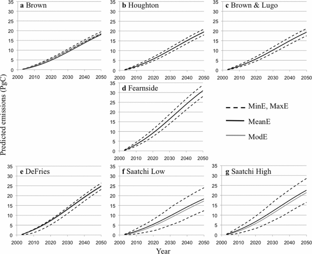
Figure 7 Carbon emissions predicted under the mean (MeanE), minimum (MinE) maximum (MaxE), and modelled (ModE) scenarios for the seven carbon maps used in the analysis (see Table 2 for a full description of maps). Vertical axis is predicted emissions (Pg of carbon) at the year represented in the horizontal axis for all seven plots. Deforestation quantity and allocation are based on the deforestation predicted by Soares-Filho et al. (Reference Soares-Filho, Nepstad, Curran, Cerqueira, Garcia, Ramos, Voll, McDonald, Lefebvre and Schlesinger2006) between 2002 and 2050.
With the exception of the Saatchi maps, DAI is marginal in most maps, to the point where the modelled and mean scenarios are visually indiscernible (Fig. 7a–e). Most DAI values are negative (Fig. 8), meaning that the simulation model of Soares-Filho et al. (Reference Soares-Filho, Nepstad, Curran, Cerqueira, Garcia, Ramos, Voll, McDonald, Lefebvre and Schlesinger2006) allocated the predicted deforestation at places that have a lower carbon density than the average in the study area. The Saatchi maps showed DAI of approximately –1.2 Pg C at their minimum, reached at year 2043 (Fig. 8). For the other maps, the minimum DAI fluctuated between –0.1 Pg C (Houghton and Brown & Lugo) and –0.3 Pg C (DeFries).

Figure 8 Influence of deforestation allocation (DAI) on the prediction of carbon emissions from deforestation based on the input carbon maps (see Table 2 for a full description of maps). DAI is calculated as carbon emissions in the modelled scenario minus the mean scenario. Negative values occur when carbon emissions in the modelled scenario are less than in the mean scenario.
We analysed the relative influence of deforestation allocation on carbon emissions among the different carbon maps (Fig. 8). For instance, DAI was similar for both the Brown and Fearnside maps until around 2020. After 2040, the DAI based on the Brown map was similar to that of the DeFries map (Fig. 8). Similarly, the Fearnside map and Brown and Lugo map become more alike after approximately 2038. DAI = 0 for the Houghton map at approximately 2025 and was trivial for the Brown and Lugo and Fearnside maps after approximately 2040. A zero DAI indicates that emissions predicted using only average carbon values are identical to emissions predicted using the projected allocation of deforestation predicted by a land change model.
DISCUSSION
Influence of quantity and allocation on the prediction of carbon emissions from deforestation
Variation in carbon quantity among carbon maps was the component with the largest influence on carbon emissions from deforestation. A larger quantity of total carbon stored in a study area represented by a particular map, implies larger predicted carbon emissions given an increase in deforestation quantity because DQI = CQ × DQ. The influence of carbon allocation on predicted emissions depends on the proportion of a study area projected as deforestation, being the largest when DQ is equal to 50% and zero when DQ is equal to 0% or 100% (Fig. 6). Carbon allocation can also be potentially influenced by CQ, since the total amount of carbon represented in a landscape determines the maximum amount of carbon that can potentially be assigned to a pixel (Fig. 2c). However, we did not find a direct relationship between CQ and CA.
The way the other three components control the influence of deforestation allocation on the prediction of carbon emissions is not conspicuous. The narrower the carbon predicting space, the more limited the range of values that DAI can adopt (Fig. 1). Based on this logic, carbon allocation might be expected to influence DAI. This seems to be the case with the Saatchi maps, which represent the largest CAI and DAI (Figs 5 and 6). Yet, the results with other carbon maps are not conclusive in this respect. Higher variability in carbon allocation does not necessarily mean a larger DAI (Figs 6 and 8), because the allocation of deforestation is not necessarily determined by the variability in carbon allocation but by the performance of the land change model.
The role of deforestation allocation on carbon emissions can be better understood by further evaluating the degree to which spatial clustering or dispersion of deforestation influences the estimation of carbon emissions. Deforestation frequently tends to occur near already deforested areas (Kirby et al. Reference Kirby, Laurance, Albernaz, Schroth, Fearnside, Bergen, Venticinque and da Costa2006). Therefore, it is possible that a land change model will not predict the exact allocation of deforestation accurately but will predict deforestation in the vicinity where carbon values will likely be similar to areas where actual deforestation occurs. Techniques such as spatial point pattern analysis (Baddeley & Turner Reference Baddeley and Turner2005) can be useful to assess the influence of patterns of deforestation allocation on the prediction of carbon emissions.
The narrow predicting space in most carbon maps (Fig. 5) denotes a low influence of carbon allocation on the prediction of carbon emissions from deforestation (see Fig. 7a–e, where the modelled scenario is nearly indistinguishable from the mean scenario, except for Saatchi maps). A larger variability in carbon allocation makes the prediction of carbon emissions more sensitive to the way deforestation is allocated. The Saatchi maps have a wider spatial variation in carbon (Figs 5 and 6) and therefore are the only ones where allocation might play a considerable role in the prediction of carbon emissions. This higher spatial variation in the Saatchi map is likely due to the representation of observed rather than potential carbon and the incorporation of additional data such as radar. The representation of observed carbon includes areas covered by secondary or degraded forests, which usually have lower carbon than the potential mature forests represented by most of the other maps. Representing lower carbon in secondary and degraded forests translates into greater spatial carbon heterogeneity compared to representing carbon in the potential vegetation. Similarly, the use of radar data improves accuracy in biomass mapping, especially in areas with low biomass densities (Gibbs et al. Reference Gibbs, Brown, Niles and Foley2007; Sanchez-Azofeifa et al. Reference Sanchez-Azofeifa, Castro-Esau, Kurz and Joyce2009), translating into greater spatial variability represented in the carbon maps.
Since carbon emissions are modelled as a function of deforestation area and carbon density, components associated with quantity should play the most relevant role in carbon emissions. However, carbon density can vary spatially and the amount of emissions depends also on the allocation of deforestation. Our results indicate the influence of allocation depends on the characteristics of the data and the procedures used for carbon mapping and the allocation of deforestation with respect to carbon. Recent advances in carbon mapping reveal important variations in carbon allocation in tropical forests that were not previously identified (Asner et al. Reference Asner, Powell, Mascaro, Knapp, Clark, Jacobson, Kennedy-Bowdoin, Balaji, Paez-Acosta, Victoria, Secada, Valqui and Highes2010). Progress in this direction will likely increase the relevance of incorporating spatial information about carbon and deforestation on the prediction of carbon emissions.
Other components influencing the prediction of carbon emissions from deforestation
We assumed that all carbon contained in a pixel was released once deforestation was predicted. However, the story may differ when predicting net rather than potential carbon emissions. A complete estimation of net carbon emissions should consider information on not only deforestation rates and carbon stocks, but also such factors as land cover dynamics following deforestation, the mode of clearing, fate of cleared carbon, historical land cover changes, and the response of soil carbon to deforestation (Houghton Reference Houghton2005; Ramankutty et al. Reference Ramankutty, Gibbs, Achard, DeFries, Foley and Houghton2007). Considering all these elements, the prediction of the spatial allocation of deforestation may play a more important role in the estimation of the timing and amount of emissions than this paper portrays, since this involves the prediction of not only allocation of deforestation, but also land conversion processes and land cover trajectories before and after clearing.
Potential applications of the method for REDD and for predicting other environmental changes
One of the main obstacles to using land change modelling to establish reference levels operationally is that it requires additional information and technical expertise, not available for all developing countries interested in REDD (Parker & Mitchell Reference Parker and Mitchell2009; GOFC-GOLD 2010). The results of this paper are specifically appropriate in assessing the potential uncertainty of developing reference levels based on the application of different tiers, meaning levels of data requirements or analytical complexity for predicting reference carbon emissions, analogous to the approach recommended by IPCC to estimate emissions or removals of greenhouse gases (Penman et al. Reference Penman, Gytarsky, Hiraishil, Irving, Krug, Eggleston, Buendia, Miwa, Ngara and Tanabe2006; Huettner et al. Reference Huettner, Leemans, Kok and Ebeling2009). Carbon stocks could be represented based on (1) default values for large geographic units (GOFC-GOLD 2010), (2) the compilation of plot data for more localized areas (for example Castillo-Santiago et al. Reference Castillo-Santiago, Hellier, Tipper and De Jong2007), or (3) through carbon mapping (Gibbs et al. Reference Gibbs, Brown, Niles and Foley2007; Olander et al. Reference Olander, Gibbs, Steininger, Swenson and Murray2008). Similarly, deforestation could be predicted by (1) considering average data on historic deforestation rates in a non spatially explicit fashion, (2) applying econometric models to predict deforestation for aggregated geographic units (for example Chomitz & Thomas Reference Chomitz and Thomas2003) or (3) through spatially explicit land change modelling (see for example Soares-Filho et al. Reference Soares-Filho, Nepstad, Curran, Cerqueira, Garcia, Ramos, Voll, McDonald, Lefebvre and Schlesinger2006).
Developing tiers for predicting emissions from deforestation would provide a useful means for countries to adjust their estimation of reference emissions levels to national circumstances, considering their data availability or technical capacity. Countries therefore could comply with the mandate by UNFCCC on establishing reference emissions levels without exclusion of any country because of data constraints or technical limitations. Countries could also opt for different tiers considering the costs associated with their implementation versus the potential benefits they could obtain from REDD, bearing in mind the uncertainty in the estimation of reference emissions levels associated with each tier. For project developers, this approach could help to bound the uncertainty of carbon emissions to areas susceptible to high deforestation (Harris et al. Reference Harris, Petrova, Stolle and Brown2008) or to improve their perceived accuracy in land change modelling by predicting the proportion of deforestation in aggregated areas with similar carbon densities.
Our approach could help to evaluate the influence of quantity and allocation on the prediction of other environmental changes. Our method may be applied to any quantitative changes that can be represented spatially and whose value is a function of deforestation or other type of spatial disturbance. The method can be used to evaluate the influence of climate change scenarios on the viability of plant populations (Miles et al. Reference Miles, Grainger and Phillips2004) and/or fauna turnover (Peterson Reference Peterson, Ortega-Huerta, Bartley, Sanchez-Cordero, Soberon and Buddemeier2002), or to analyse the sensitivity of predicted nitrogen retention and deposition on the quantity and spatial distribution of climate, forest types and anthropogenic land changes (Pan et al. Reference Pan, Hom, Birdsey and McCullough2004; Fedorko et al. Reference Fedorko, Pontius, Aldrich, Claessens, Hopkinson and Wolheim2005).
CONCLUSIONS
The prediction of carbon emissions from deforestation should consider the interacting effects of quantity and allocation in deforestation and carbon maps. We examined case studies where the components associated with quantity of existing carbon and quantity of future deforestation are more influential than the spatial allocation of those quantities.
This paper offers a novel approach to assessing the influence of spatial and non-spatial components of uncertainty associated with carbon mapping and land change modelling on the prediction of carbon emissions from deforestation. Our method is particularly suitable for the establishment of reference emission levels for REDD or other carbon mitigation projects based on different tiers (levels) of data input, and may also be applied to predict other environmental changes affected by spatial disturbances.
ACKNOWLEDGEMENTS
Victor Hugo Gutierrez-Velez was supported by a Clark University fellowship in Geographic Information Sciences for Development and Environment, and received financial support from NSF award number 0909475 and COLCIENCIAS while writing this paper. Drs Richard Houghton, Sandra Brown and Joe Hackler provided some of the carbon maps used in the analysis. We thank Allison Hayes-Conroy, Douglas Morton, Carlos Sierra and Marcia Macedo for providing valuable insights that helped improve the paper. We are also grateful to the editors and reviewers for their helpful comments. Clark Labs facilitated this work by creating and making available the GIS software Idrisi®.


