


1. Introduction
Climate change is likely to have a wide range of impacts in both developed and developing countries. In the fifth assessment report by the IPCC (Intergovernmental Panel on Climate Change), the international community has accepted the main mechanisms relating emissions and atmospheric CO2 concentration to the rise in global mean temperature. With a growing consensus that the global warming is happening and it is mainly due to anthropogenic emissions of greenhouse gases (GHGs), the international community has agreed on the need for joint action to limit GHG emissions. However, current international cooperation has not been effective (Finus and Pintassilgo, Reference Finus and Pintassilgo2013). One important problem is free riding, given that climate stability is a global public good (see, e.g., Hoel, Reference Hoel1993; Wirl, Reference Wirl1996). Unless there is binding international law which forces countries to participate in an agreement to reduce GHG emissions, each country can choose to stay outside the agreement and enjoy (almost) the same benefits of reduced GHGs emissions as if it participated in the agreement, while it doesn't bear any of the costs of reducing emissions (Hoel, Reference Hoel1993).
In addition to the free-riding problem, it has been argued that the huge uncertainties surrounding climate change can be one of the reasons for the lack of cooperation (see, e.g., Kolstad, Reference Kolstad2007; Barrett and Dannenberg, Reference Barrett and Dannenberg2012; Finus and Pintassilgo, Reference Finus and Pintassilgo2013). Due to these uncertainties, it is almost impossible to know the exact effects of one more unit of GHG emissions today on global temperature, and thus damage, in the future. This could make individual countries hesitant about investing in emission abatement and cooperating with other countries. For instance, uncertainty was one of the arguments used by former US President George W. Bush for his decision to pull the US out of the Kyoto Protocol. As quoted by Kolstad (Reference Kolstad2007), President Bush wrote in a letter to senators: ‘I oppose the Kyoto Protocol … we must be very careful not to take actions that could harm consumers. This is especially true given the incomplete state of scientific knowledge.’ (See also Finus and Pintassilgo, Reference Finus and Pintassilgo2013).
If climate uncertainty could reshape the abatement strategies of individual countries, this might also have an effect on their expected welfare. However, these effects might be different depending on whether the countries cooperate with each other. This implies that uncertainty could have an impact on the potential welfare gains from cooperation for individual countries, thereby affecting the incentives for cooperation among countries. Therefore, it is important to investigate whether this would be true in a normative perspective and to see in precisely what way dealing with uncertainty could reshape climate policies and change the incentives for international cooperation on climate change.
In this paper, we extend the deterministic dynamic game for international pollution control in Dockner and Long (Reference Dockner and Long1993) to study the welfare gain from international cooperation under climate uncertainty. We analytically compare the cooperative and non-cooperative solutions of the game with the aim of answering the following questions. How does uncertainty about global warming affect the net welfare of individual countries in the respective non-cooperative and cooperative cases? How does climate uncertainty affect the benefits (welfare gains) from international cooperation (and thus the side payments among countries)? By focusing on players’ payoffs under uncertainty, we show that the expected payoffs of players decrease as climate uncertainty becomes greater, whether or not they cooperate. However, the expected welfare gain from international cooperation is larger with greater climate uncertainty, implying that it is more important to cooperate when facing greater uncertainty. At the same time, however, more transfers will be needed to ensure stable cooperation among asymmetric players.
There are numerous studies on climate uncertainty and its effect on climate policy design. Some authors investigated the optimal timing to slow global warming under uncertainties (see, for instance, Conrad, Reference Conrad1997; Pindyck, Reference Pindyck2000; Pindyck, Reference Pindyck2002; Bahn et al., Reference Bahn, Haurie and Malhamé2008), the value of learning for climate change uncertainties (e.g., Peck and Teisberg, Reference Peck and Teisberg1993; Kolstad, Reference Kolstad1996; Kelly and Kolstad, Reference Kelly and Kolstad1999), the optimal choice of policy instruments to mitigate climate change in the presence of uncertainty (e.g., Pizer, Reference Pizer1999, Reference Pizer2002; Hoel and Karp, Reference Hoel and Karp2001, Reference Hoel and Karp2002), and the strategic interactions between producers of fossil fuels and a taxing government concerned about consumers’ welfare under climate uncertainty (e.g., Wirl, Reference Wirl2007). Moreover, literature on the effect of uncertainty (and learning) on international cooperation has emerged recently (for instance, Kolstad, Reference Kolstad2007; Kolstad and Ulph, Reference Kolstad and Ulph2008, Reference Kolstad and Ulph2011; Barrett and Dannenberg, Reference Barrett and Dannenberg2012; Karp, Reference Karp2012; Finus and Pintassilgo, Reference Finus and Pintassilgo2013). Notably, Harstad (Reference Harstad2016) investigates the harmful (short-term) climate agreements and optimal (long-term) agreement taking into account uncertainty. Battaglini and Harstad (Reference Battaglini and Harstad2016) studies the participation and duration of international environmental agreements in a dynamic game in which countries pollute and invest in green technologies when the contract is incomplete. Bréchet et al. (Reference Bréchet, Thénié, Zeimes and Zuber2012) numerically examines the benefits of international climate cooperation under uncertainty through a stochastic integrated assessment model, finding that uncertainty generates additional benefit from cooperation, namely risk reduction.
The closest papers to ours are those by (Xepapadeas, Reference Xepapadeas1998, Reference Xepapadeas, Hahn and Ulph2012) and Wirl (Reference Wirl2008). Like us, they analyze non-cooperative versus cooperative solutions. Their focus, however, is different. Xepapadeas (Reference Xepapadeas1998) studies optimal policy adoption rules of emission abatement for cooperative and non-cooperative solutions under uncertainty about global warming damages, while Wirl (Reference Wirl2008) focuses on how uncertainty affects pollution control strategies in cooperative and non-cooperative solutions for both irreversible emissions and reversible emissions. Finally, Xepapadeas, (Reference Xepapadeas, Hahn and Ulph2012) focuses on the cost of ambiguity and robustness in international pollution control when the regulator has concerns regarding possible misspecification of the natural system that is used to model pollution dynamics. Moreover, by limiting their analysis to players who are symmetric in terms of benefits and damages, these studies ignore the heterogeneity among players in terms of optimal emission strategies and total payoffs and thus the analysis on welfare transfers between players is omitted (see, e.g., Wirl, Reference Wirl2008; Xepapadeas, Reference Xepapadeas, Hahn and Ulph2012). We analyze the results for both the case of symmetric players and the case of asymmetric players, and investigate the side payments that are needed to ensure stability of the cooperation.
The contribution of this paper is as follows. First, we use a stochastic dynamic game with climate uncertainty and analyze the effect of climate uncertainty on the players’ payoffs rather than on the effect on emissions strategies only and this allows us to further examine the effect of uncertainty on the benefits of international cooperation. Second, we analytically and numerically investigate the effect of uncertainty taking into account the asymmetry of players (countries) whereas most of the extended transboundary pollution control models for incorporating uncertainty in the literature assume the symmetry of players (see, e.g., Wirl, Reference Wirl2008; Xepapadeas, Reference Xepapadeas, Hahn and Ulph2012). Last but not least, we also investigate the possible transfers among players to ensure cooperation and how they would change with climate uncertainty.
The paper is organized as follows. Section 2 presents the stochastic dynamic game. Section 3 presents the non-cooperative and cooperative solutions of the game. The effects of climate uncertainty under the cases of symmetric players and asymmetric players are analyzed in sections 4 and 5, respectively. Section 6 provides some numerical illustrations. Finally, section 7 concludes the paper. Some proofs are relegated to an online appendix.
2. The model
The deterministic part of the game is based on the international pollutant control model developed by Dockner and Long (Reference Dockner and Long1993). As in that paper, we assume that there are two countries (indexed by i=1, 2) and a single consumption good in the world. The production of the consumption good in country i results in CO2 emissions E i:
 $$Y_{i} = F_{i}(E_{i}),$$
where Y i is the output in country i. Both countries’ emissions contribute to global warming. The future temperature (measured in °C above the pre-industrial average) is stochastic due to the uncertainty of the climate system.Footnote 1 Following the specification for climate uncertainty in Wirl (Reference Wirl2007), the global mean temperature is assumed to follow the Ito process:
 $$dT(t)=[E_{1}(t)+E_{2}(t)]dt + \sigma T(t)dz,T(0) = T_{0}\geq0,$$
where E i(t) is measured in units that lead to an expected increase of global average temperature by 1°C. It can be seen from (1) that the expected temperature will be determined by the accumulation of CO2 emissions in the atmosphere and that the stochastic part of the temperature is a geometric Brownian motion (σ>0 is the relative standard error and z is a standard Wiener process).Footnote 2 As in Wirl (Reference Wirl2007), the parameter σ can be considered a measurement of the degree of (relative) uncertainty. A larger σ would imply a greater degree of uncertainty.
Country i enjoys utility/benefit U i(Y i) from consumption but suffers damage from global warming D i(T). As in Dockner and Long (Reference Dockner and Long1993) and its follow-ups, U i(·) and D i(·) have quadratic forms (which are prevailing in the literature, see, e.g., Wirl, Reference Wirl2008; Xepapadeas, Reference Xepapadeas, Hahn and Ulph2012) such that country i gets the normalized utility from consumption  $U_{i}(F_{i}(E_{i}(t))) = a_{i}E_{i}(t) - {[E_{i}(t)]^{2}}/{2}$ and faces the damage of global warming
  $D_{i}(T(t)) = {\varepsilon_{i}}/{2}[T(t)]^{2}$, where a i and εi are positive constants. The net benefit/utility for country i is therefore:
 $$B_{i}(E_{i}(t),T(t)) = a_{i}E_{i}(t) - {1 \over 2}[E_{i}(t)]^{2} - {\varepsilon_{i} \over 2}[T(t)]^{2}.$$
Without loss of generality, we set a 1=a, and a 2=φa; ε1=ε, and ε2=γε. Note that if φ=1 and γ=1, the two countries have symmetric benefits and damages.
Without cooperation between the two countries, country i will choose CO2 emissions E i to maximize its discounted stream of net benefits from consumption:
 $${\open E}\int_{0}^{\infty}e^{-rt} \left\{a_{i}E_{i}(t) - {1 \over 2} [E_{i}(t)]^{2}- {\varepsilon_{i} \over 2}[T(t)]^{2}\right\}dt,$$
subject to the global temperature dynamics (1). r is the discount rate, which is assumed to be the same for both countries. The expectation sign  ${\open E}(\cdot)$ appears due to the uncertainty of global warming implied in (1). Therefore, we have a stochastic dynamic game in which the dynamics of global mean temperature involve uncertainty. As in Wirl (Reference Wirl2007), it is further assumed that σ2<r, which will ensure that the net present value of expected damage remains finite. As we shall see in section 3 below, the solution concept used for the game would be Markov-perfect Nash equilibrium.
With cooperation between countries, the two countries will jointly maximize the joint net benefit stream (by choosing the CO2 emissions in the two countries: E 1 and E 2) which is the sum of each country's net benefit:Footnote 3
 $${\open E}\int_{0}^{\infty}e^{-rt}\left\{ a[E_{1}(t)+\varphi E_{2}(t)]- {1 \over 2}[ [E_{1}(t)]^{2}+[E_{2}(t)^{2}]] - {\varepsilon(1+\gamma) \over 2}[T(t)]^{2}\right\} dt,$$
subject to the global temperature dynamics (1). The solution of the cooperative game can be considered as a first-best outcome where the countries are able to achieve an agreement for emission control. Therefore, one can get some insights into the benefits (welfare gains) from international cooperation for individual countries by comparing their payoffs under cooperative strategies with those under non-cooperative strategies. As can be noted in the model setup, we do not impose non-negativity (or irreversibility) constraints on the control variables, implying that emissions are assumed to be reversible. That is, active but costly reduction of the stock of emissions (cleanup) is assumed to be feasible.Footnote 4 As argued by Xepapadeas (Reference Xepapadeas, Hahn and Ulph2012), though there are many cases in pollution control where a more realistic assumption would be to impose the non-negativity constraint, the irreversibility can be considered as a consequence of the policymaker's inability to reduce the stock of pollution, and without the non-negativity constraint low emissions just have no option value since cleanup is possible. Therefore, we follow Xepapadeas (Reference Xepapadeas, Hahn and Ulph2012) and do not consider the emission irreversibility in this paper.Footnote 5
3. Non-cooperative and cooperative solutions
In this section, we derive the solution of the game for the non-cooperative and cooperative case, respectively. Compared with an open-loop Nash equilibrium, a Markov-perfect Nash equilibrium is more informative because it provides a subgame perfect equilibrium that is dynamically consistent. Therefore, we assume that players are playing Markovian strategies rather than open-loop strategies. Markovian strategies imply that each player will choose an emission strategy at time t based on the state of the system (i.e., temperature T) at that time.
3.1 Non-cooperative case
Define the value function for player i when the players do not cooperate as V i (T). Then, the Markovian strategies of player 1 and player 2, E 1 (T) and E 2 (T), need to satisfy the following Hamilton-Jacobi-Bellman (HJB) equations:
 $$rV_{1}(T) = \max\limits_{E_{1}}\left\{ aE_{1}- {1\over 2} [E_{1}]^{2}- {\varepsilon \over 2}T^{2}+[E_{1}+E_{2}(T)]\cdot V_{1}^{\prime}(T)+\left({1 \over 2}\sigma^{2}T^{2}\right)V_{1}^{\prime \prime}(T)\right\}$$
 $$rV_{2}(T) = \max\limits_{E_{2}} \left\{a\varphi E_{2}\,{-}\, {1\over 2}[E_{2}]^{2}\,{-}\,{\gamma\varepsilon \over 2}T^{2}\,{+}\,[E_{1}(T)\,{+}\,E_{2}] \cdot V_{1}^{\prime}(T)\,{+}\left({1 \over 2}\sigma^{2}T^{2}\right) V_{2}^{\prime \prime}(T)\right\},$$
where  $V_{i}^{\prime}\,(T)$ and
  $V_{i}^{\prime\prime}\,(T)$ are the first- and second-order derivatives of the value function V i(T) with respect to the state variable, i.e., global temperature T. The second derivatives of the value functions appear due to the stochastic nature of the problem (Dockner et al., Reference Dockner2000).
From the first-order conditions for the maximization of the right-hand side of HJB equations (4a) and (4b), one can find the optimal emission strategy for the two players as:
 $$E_{1}(T) = a + V_{1}^{\prime}(T)$$
 $$E_{2}(T) = a \varphi + V_{2}^{\prime}(T).$$
Equations (5a) and (5b) state that players’ optimal emission strategy would depend on the instantaneous marginal benefits of more emissions and also the marginal intertemporal effect. Plugging (5a) and (5b) into the HJB equations (4a) and (4b), and after some straightforward calculations, one can obtain:
 $$rV_{1}(T) = {1 \over 2}[a + V_{1}^{\prime}(T)]^{2}- {\varepsilon \over 2} T^{2}+[a\varphi + V_{2}^{\prime}(T)]\cdot V_{1}^{\prime}(T)+\left({1 \over 2} \sigma^{2}T^{2}\right)V_{1}^{\prime\prime}(T)$$
 $$rV_{2}(T) = {1 \over 2}[\varphi a+V_{2}^{\prime}(T)]^{2}- {\gamma \varepsilon \over 2} T^{2} + [a+V_{1}^{\prime}(T)]\cdot V_{2}^{\prime}(T) + \left({1 \over 2}\sigma^{2}T^{2} \right) V_{2}^{\prime\prime}(T).$$
Due to the linear-quadratic structure of the game, we know the value function is quadratic:
 $$V_{i}(T) = \kappa_{i} + \mu_{i}T + {1 \over 2} \eta_{i}T^{2},i = 1,2,$$
where κi, μi, ηi are the coefficients to be determined. Substituting (7) into (6a) and (6b), we have:
 $$\eqalign{r\left[\kappa_{1} + \mu_{1}T + {1 \over 2} \eta_{1}T^{2}\right] &= {1 \over 2}[a+\mu_{1} + \eta_{1}T]^{2} \cr &\quad +[\varphi a + \mu_{2} + \eta_{2}T][\mu_{1} + \eta_{1}T] - {\varepsilon \over 2}T^{2} + {\sigma^{2}T^{2} \over 2}\eta_{1}}$$
 $$\eqalign{r\left[\kappa_{2}+\mu_{2}T + {1 \over 2}\eta_{2}T^{2}\right] &= {1 \over 2}[\varphi a + \mu_{2} \cr &\quad+\eta_{2}T]^{2}+[a+\mu_{1}+\eta_{1}T][\mu_{2}+\eta_{2}T]-{\gamma\varepsilon \over 2}T^{2} + {\sigma^{2}T^{2} \over 2}\eta_{2}.}$$
Equating the coefficients of 1, T and T 2 on both sides of (8a) and (8b) leads to the following system of equations:
 $${1 \over 2}r\eta_{1} = {1 \over 2}[\eta_{1}]^{2}+\eta_{1}\eta_{2} - {\varepsilon \over 2} + {\sigma^{2} \over 2}\eta_{1}$$
 $$r\mu_{1} = [a + \mu_{1}] \eta_{1} + \eta_{2}\mu_{1} + \eta_{1} [\varphi a + \mu_{2}]$$
 $$r\kappa_{1} = {1 \over 2}[a + \mu_{1}]^{2} + [\varphi a + \mu_{2}]\mu_{1}$$
 $${1 \over 2} r \eta_{2} = {1 \over 2} [\eta_{2}]^{2} + \eta_{1}\eta_{2} - {\gamma\varepsilon \over 2} + {\sigma^{2} \over 2}\eta_{2}$$
 $$r\mu_{2} = [\varphi a+\mu_{2}]\eta_{2}+\eta_{1}\mu_{2}+\eta_{2}[a+\mu_{1}]$$
 $$r\kappa_{2} = {1 \over 2}[\varphi a+\mu_{2}]^{2}+[a+\mu_{1}]\mu_{2}.$$
By solving the system of equations (9a)–(9f), one can determine the coefficients for the value function V i(T), i=1, 2. However, it should be emphasized that the general case (with arbitrary values of φ and γ) does not allow for explicitly analytical solutions of (9a)–(9f). Therefore, our analysis will concentrate on some cases where analytical results are possible, as we shall see in sections 4 and 5 below.
3.2 Cooperative case
As mentioned above, in the cooperative case, the two countries will jointly choose E 1 and E 2 to maximize (3), subject to the global temperature dynamics (1). If we define the value function in this case as W(T), the following HJB equation can be obtained:
 $$\eqalign{rW(T) &= \max\limits_{E_{1},E_{2}}\{a[E_{1} + \varphi E_{2}] - {1 \over 2}[(E_{1})^{2}+(E_{2})^{2}]- {(1+\gamma)\varepsilon \over 2}T^{2}\cr &\quad+[E_{1} + E_{2}]\cdot W^{\prime}(T) + {1 \over 2}\sigma^{2}T^{2}W^{\prime\prime} (T) \}.}$$
The first-order conditions for the maximization of the right-hand side yield:
 $$E_{1}(T) = a + W^{\prime}(T)$$
 $$E_{2}(T) = a \varphi + W^{\prime}(T).$$
Similarly to the non-cooperative case (equations (5a) and (5b)), it can be seen from equations (11a)–(11b) that the players’ optimal emission strategy in the cooperative case also depends on both the instantaneous marginal benefits of emissions and the marginal intertemporal effect. Plugging (11a)–(11b) into the HJB equation (10), after some calculations we have:
 $$\eqalign{rW(T) &= \left[W^{\prime}(T)+ {a(1+\varphi) \over 2}\right]^{2}\cr &\quad+ {a^{2}(1-\varphi)^{2} \over 4}- {\varepsilon(1+\gamma) \over 2}T^{2} + \left({1 \over 2}\sigma^{2} T^{2}\right)W^{\prime\prime}(T).}$$
Again, we know the value function is in a quadratic form:
 $$W(T) = \zeta + \psi T + {1 \over 2} \xi T^{2},$$
where ζ, ψ, and ξ are the coefficients to determine. Plugging (13) into (12), we have:
 $$\eqalign{r[\zeta + \psi T + {1 \over 2}\xi T^{2}] &= [\psi + \xi T]^{2} + a(1 + \varphi)[\psi + \xi T]\cr &\quad+ {a^{2}(1+\varphi^{2}) \over 2} - {\varepsilon(1+\gamma) \over 2}T^{2} + {1 \over 2}\sigma^{2}T^{2}\xi.}$$
Equating the coefficients on both sides, one can get the following system of equations:
 $${1 \over 2}r \xi = \xi^{2} - {\varepsilon(1 + \gamma) \over 2} + {\xi \sigma^{2} \over 2}$$
 $$r\psi = 2 \psi \xi + a(1 + \varphi)\xi$$
 $$r\zeta = \psi^{2} + a(1 + \varphi) \psi + {a^{2}(1+\varphi^{2}) \over 2},$$
from which one can obtain:
 $$\xi = {(r-\sigma^{2})-\sqrt{(r-\sigma^{2})^{2}+8\varepsilon(1+\gamma)} \over 4}$$
 $$\psi = {a(1+\varphi) \xi \over r - 2\xi} = \displaystyle{1 \over 2}\left[\displaystyle{ar(1 + \varphi) \over (r-2\xi)} - a(1 + \varphi) \right]$$
 $$\zeta = \displaystyle{1 \over r} \left[\psi + \displaystyle{a(1 + \varphi) \over 2}\right]^{2} + \displaystyle{a^{2} (1-\varphi)^{2} \over 4r}.$$
We have thereby determined the coefficients for the value function W(T). While the effect of uncertainty σ will be investigated later on, the effect of some other parameter can also be seen from (16a)–(16c). For instance, it is straightforward to find that the sign of  ${\partial \xi \over \partial \gamma}$ is negative, which implies that (together with equations (11a) and (11b)) the optimal emissions will decrease with temperature more dramatically when the damage from climate change for country 2 becomes higher (i.e., a larger γ), which is consistent with the expectation.
4. The case of symmetric players
In this section, we investigate the game described above under the assumption that the two countries are symmetric in benefits from emissions and damages from global warming, i.e., φ=1 and γ=1.
4.1 Expected payoffs
Due to the symmetry of the two countries, both countries will achieve the same payoff in the equilibrium, which implies that the value function in the non-cooperative solution would be identical for both countries, i.e., V 1(T)=V 2(T)=V(T), implying that the coefficients of the value functions V 1(T) and V 2(T) satisfy κ1=κ2=κ, μ1=μ2=μ, and η1=η2=η. Therefore, the symmetry of the two countries would imply that (9a)–(9f) can be degenerated as:
 $$\displaystyle{1 \over 2}r \eta = \displaystyle{1 \over 2}[\eta]^{2} + [\eta]^{2} - \displaystyle{\varepsilon \over 2} + \displaystyle{\sigma^{2} \over 2}\eta$$
 $$r\mu = [a + \mu]\eta + \eta \mu + \eta [a + \mu]$$
 $$r\kappa = \displaystyle{1 \over 2} [a + \mu]^{2} + [a + \mu]\mu.$$
 By solving this system of equations, one can determine the coefficients for the value function V(T), as in the first column of table 1.Footnote 6 Given the initial temperature T 0, the (expected) payoff for each country in the non-cooperative case will be  $V^{NC}(T_{0}) = V(T_{0}) = \kappa + \mu T_{0} + {1 \over 2} \eta [T_0]^{2}$.
Table 1. Coefficients for value functions in the case of symmetric players

Similarly, with the symmetric players, the coefficients for the value function under cooperation, W(T), i.e., (16a)–(16c), would degenerate into the second column of table 1.
4.2 Non-cooperative versus cooperative strategies
In the case of symmetric players, the emission strategies of the two players would be identical, as can be seen from (5a) and (5b). Taking into account the expression of the value function, one can obtain the optimal emission strategy for each country in the non-cooperative case:
 $$E_{i}^{NC}(T) = a + \mu + \eta T,$$
and the optimal emission strategy for country i in the cooperative case:
 $$E_{i}^{C}(T) = a + \psi + \xi T,$$
where μ, η, ψ, and ξ are as in table 1.
In the online appendix A1, we show that ξ−η<0 and ψ−μ<0. Therefore, for the same temperature T, we have  $E_{i}^{C}(T) \lt E_{i}^{NC}(T)$. That is, each country tends to over-emit CO2 in the non-cooperative case, compared with the cooperative case. If we denote the temperatures at which countries would stop emitting (i.e., would have zero emissions) for the non-cooperative and cooperative cases as
  $\bar{T}^{NC}$ and
  $\bar{T}^{C}$, respectively, we have:
  $\bar{T}^{NC} = {a + \mu}/-\eta$ and
  $\bar{T}^{C} = {a + \psi}/{-\xi}$. Because
  $0 \lt \psi + a \lt \mu + a$ and ξ<η<0 (see table 1 and online appendix A1), we have
  $\bar{T}^{NC} \gt \bar{T}^{C} \gt 0$. That is, countries will stop emissions at a lower temperature under international cooperation.This result is consistent with the general findings in the literature (e.g., Dockner and Long, Reference Dockner and Long1993; Wirl, Reference Wirl2008).Footnote 7
Moreover, in online appendix A2 we show that  ${\partial \eta}/ {\partial \sigma} \lt 0$,
  ${\partial \mu}/{\partial \sigma} \lt 0$,
  ${\partial \xi}/{\partial \sigma} \lt 0$ and
  ${\partial \psi}/{\partial \sigma} \lt 0$, which implies that
  ${\partial E_{i}^{NC}(T)}/{\partial \sigma} = {\partial \mu}/{\partial \sigma} + {\partial \eta}/{\partial \sigma}T \lt 0$ and
  ${\partial E_{i}^{C}(T)}/{\partial \sigma} = {\partial \psi}/ {\partial \sigma} + {\partial \xi}/{\partial \sigma}T \lt 0$ for a given temperature T≥0. That is, uncertainty will make countries more cautious about their emissions, whether they cooperate or not. This is consistent with the previous findings on the consequences of uncertainty in the context of the tragedy of the commons (see, e.g., Wirl, Reference Wirl2008): larger uncertainty reduces pollution. However, in contrast to the previous studies, the focus of this paper is on the effects of climate uncertainty on the welfare of individual countries in non-cooperative as well as cooperative solutions and on the welfare gain from international cooperation. Therefore, more emphasis will be put on the effects of uncertainty on these measurements in the following sections.
4.3 Effect of uncertainty on the welfare of individual countries
Due to the symmetry of players, both countries achieve the same payoff  $V^{NC} (T_{0}) = V(T_{0})$ in the non-cooperative case, while both also obtain the same payoff
  $V^{C} (T_{0}) = {1}/{2} W(T_{0})$ in the cooperative case, where T 0 is the initial temperature. To see the effect of uncertainty on an individual country's welfare, let us take the derivative of V NC (T 0) and V C (T 0) with respect to the parameter σ, which is the measurement of climate uncertainty. That is,
 $$\displaystyle{\partial V^{NC}(T_{0}) \over \partial \sigma} = \displaystyle{\partial \kappa \over \partial \sigma} + \displaystyle{\partial \mu \over \partial \sigma} T_{0} + \displaystyle{1 \over 2} \displaystyle{\partial \eta \over \partial \sigma}[T_{0}]^{2}$$
 $$\displaystyle{\partial V^{C} (T_{0}) \over \partial \sigma} = \displaystyle{1 \over 2} \displaystyle{\partial \zeta \over \partial \sigma} + \displaystyle{1 \over 2} \displaystyle{\partial \psi \over \partial \sigma} T_{0} + \displaystyle{1 \over 4} \displaystyle{\partial \xi \over \partial \sigma} [T_{0}]^{2}.$$
Based on the coefficients of value functions in table 1, the following results can be established and demonstrated for the case with symmetric players.
Proposition 1
Larger climate uncertainty reduces the expected welfare of individual countries, whether or not they cooperate with each other.
Proof: Since it has been shown in online appendix A2 that  ${\partial\eta}/{\partial\sigma}\lt 0$,
  ${\partial\mu}/{\partial\sigma} \lt 0$, and
  ${\partial\kappa}/{\partial\sigma} \lt 0$, one can know that
  ${\partial V^{NC}(T_{0})}/{\partial \sigma} = {\partial \kappa}/ {\partial \sigma} + {\partial \mu}/{\partial \sigma} T_{0} + {1}/{2} {\partial \eta}/ {\partial \sigma}[T_{0}]^{2} \lt 0$ for T 0≥0, which implies that, in the non-cooperative case, the expected payoff for each country will be reduced by greater uncertainty about global warming. Similarly, the negative signs of
  ${\partial \xi} / {\partial \sigma}$,
  ${\partial \psi}/{\partial \sigma}$, and
  ${\partial \zeta}/ {\partial \sigma}$ (see the proofs in online appendix A2) imply
  ${\partial V^{C}(T_{0})}/{\partial \sigma} = {1}/{2}{\partial \zeta}/{\partial \sigma} + {1}/{2}{\partial \psi}/{\partial \sigma} T_{0} + {1}/{4} {\partial \xi}/{\partial \sigma} [T_{0}]^{2} \lt 0$ for T 0≥0. That is, the expected payoff for each country will be reduced by greater climate uncertainty in the cooperative case as well. Therefore, we know that, no matter whether or not the two countries cooperate with each other, higher uncertainty about global warming will reduce the expected welfare of individual countries. □
4.4 Effect of uncertainty on benefits of international cooperation
The welfare gain from international cooperation (WGIC) for each country can be calculated as the difference between the payoff in the cooperative case and that in the non-cooperative case:
 $$\eqalign{WGIC &= V^{C}(T_{0}) - V^{NC}(T_{0})\cr &= \left(\displaystyle{1 \over 2} \zeta + \displaystyle{1 \over 2} \psi T_{0} + \displaystyle{1 \over 4} \xi [T_{0}]^{2} \right) - \left(\kappa + \mu T_{0} + \displaystyle{1 \over 2} \eta [T_{0}]^{2} \right) \cr &= \left(\displaystyle{1 \over 2} \zeta - \kappa \right) + \left(\displaystyle{1 \over 2} \psi - \mu \right) T_{0} + \displaystyle{1 \over 2} \left(\displaystyle{1 \over 2} \xi - \eta \right) [T_{0}]^{2}.}$$
It is well known that collective well-being can be increased if all countries cooperate in managing shared environmental resources such as the climate and ozone layer (Barrett, Reference Barrett1994). This implies that one can always expect that the two players’ combined payoff in the cooperative case would be larger than that in the non-cooperative case. Taking into account the symmetry of the two players (an equal split of the collective payoff), this leads to:
Lemma 1
It is always beneficial for the countries to cooperate, no matter how large the climate uncertainty is.
Though Lemma 1 directly follows from well-known general economics results, one can rigorously prove that this is true in our particular case by some straightforward calculations. In online appendix A3, we demonstrated that 1/2ζ−κ>0, 1/2ψ−μ>0, and 1/2ξ−η>0 hold for all σ (under the assumption that σ2<r). Therefore, we know from equation (20) that the welfare gain from cooperation for each country (for a given initial temperature T 0≥0) is positive for all σ. That is, each country can always get a positive welfare gain from international cooperation, no matter how large the uncertainty is.
We know that the expected welfare gain from international cooperation is positive (Lemma 1). But how will the size of the welfare gain from cooperation change with climate uncertainty? To see this, take the derivative of WGIC (see (20)) with respect to σ:
 $$\displaystyle{\partial WGIC \over \partial \sigma} = \left(\displaystyle{1 \over 2} \displaystyle{\partial \zeta \over \partial \sigma} - \displaystyle{\partial \kappa \over \partial \sigma} \right) + \left(\displaystyle{1 \over 2} \displaystyle{\partial \psi \over \partial \sigma} - \displaystyle{\partial \mu \over \partial \sigma} \right) T_{0} + \displaystyle{1 \over 2} \left(\displaystyle{1 \over 2} \displaystyle{\partial \xi \over \partial \sigma} - \displaystyle{\partial \eta \over \partial \sigma} \right) [T_{0}]^{2}.$$
 As we shall state in Proposition 2, one can demonstrate that  ${\partial WGIC}/{\partial\sigma} \gt 0$, which implies that the expected welfare gain from cooperation for each country (i.e., WGIC) is increasing in the magnitude of climate uncertainty (i.e., increasing in parameter σ).
Proposition 2
The expected WGIC is an increasing function of climate uncertainty. The larger the uncertainty, the more each country can gain from cooperation.
Proof See online appendix A4. □
Proposition 2 highlights one of the most important findings of this study. The economic intuition behind this is as follows: An increasing σ implies that the random variations in temperature T caused by the diffusion term σT(t)dz, representing the risk involved in emitting GHGs, is increasing. This increase in risk increases the countries’ expected shadow costs of temperature  ${\partial V_{i}}/{\partial T}$ in the non-cooperative case relatively more than the expected shadow cost
  ${\partial W}/{\partial T}$ in the cooperative case. This is derived from the fact that in the non-cooperative case the countries individually maximize their expected net benefit streams, thus facing lower expected shadow costs of temperature and leading to higher optimal emissions level and higher temperature, compared to the case when two countries maximize the joint expected net benefit stream in the cooperative case. Consequently, the expected value of discounted net benefit to each country in the non-cooperative case decreases relatively more than the expected value of discounted net benefits in the cooperative case as σ increases.
Given 1/2ψ−μ>0 and 1/2ξ−η>0 (see online appendix A3), it is easy to show that:  ${\partial WGIC}/{\partial T^{0}} = (1/2 \psi - \mu) + (1/2 \xi - \eta) [T_{0}] \gt 0$ for T 0≥0, which implies the expected WGIC for each country is increasing in the initial global temperature T 0 as well. That is, the importance of international cooperation increases with a higher initial temperature: the higher the initial temperature, the more important it is to have international cooperation. The intuition is that the climate damage increases in temperature, thereby making the emissions in the cooperative case (relative to the emissions in the non-cooperative case) become even more conservative when the temperature is higher.
5. The case of asymmetric players
We focused on the case of symmetric players in the previous section. However, in reality, countries are asymmetric: some countries are affected a lot by climate change, while others are affected less; the benefits from emissions can also be very different. Therefore, it is important to investigate the case of asymmetric players. The case of asymmetric players corresponds to the case where φ≠1 or/and γ≠1. As mentioned in section 3, the general (asymmetric) case (with arbitrary value of φ and γ) does not allow for an explicitly analytical solution of the non-cooperative game. Therefore, following List and Mason (Reference List and Mason2001), let us focus the analysis with asymmetric players on a polar extreme case where γ=0, which represents the extreme case in which country 2 does not suffer from the environmental damage of global warming.
5.1 Expected payoffs
If we assume γ=0, it is easy to see that the optimal emission strategy of country 2 in the non-cooperative case is to set E 2(T)=ϕa, which implies country 2 is not a strategic player anymore in this case, i.e., at each instant of time, country 2 will receive the instantaneous net benefit B 2=1/2(φa)2. In other words, we would have  $\kappa _{2}={1}/{2r}(\varphi a)^{2}$, μ2=0, and η2=0 in the value function for country 2,
  $V_{2}(T) = \kappa_{2} + \mu_{2}T + {1}/{2}\eta_{2} T^{2}$. If one plugs in the values of κ2, μ2, and η2, equations (9a)–(9c) become:
 $$\displaystyle{1 \over 2} r\eta_{1} = \displaystyle{1 \over 2} [\eta_{1}]^{2} - \displaystyle{\varepsilon \over 2} + \displaystyle{\sigma^{2} \over 2}\eta_{1}$$
 $$r\mu_{1} = [a + \mu_{1}] \eta_{1} + \varphi a \eta_{1}$$
 $$r\kappa_{1} = \displaystyle{1 \over 2} [a + \mu_{1}]^{2} + \varphi a \mu_{1}.$$
From this system of equations, one can solve for η1, μ1, and κ1, as shown in the first column in table 2. With the assumption of γ=0, the coefficients for the value function under cooperation W(T), i.e., (16a)–(16c), degenerate into the third column of table 2. It can be observed from table 2 that the following relations hold:
 $$2\xi - \eta_{1} = {-\sqrt{(r - \sigma^{2}) + 8\varepsilon} + \sqrt{(r - \sigma^{2})^{2} + 4\varepsilon} \over 2} \lt 0$$
 $$2\psi - \mu_{1} = {a(1 + \varphi)[r(2\xi - \eta_{1})] \over (r - 2\xi)(r - \eta_{1})} \lt 0.$$
Table 2. Coefficients for value functions in the particular case of asymmetric players

5.2 Non-cooperative versus cooperative strategies
Recall that, without the constraint of cooperation, country 2 will behave non-strategically and the optimal emission strategy for country 2 is always to set E 2NC (T)=φa. For country 1, the optimal emission strategy under non-cooperation in this case, plugging the value function V 1 (T) into (5a), is:
 $$E_{1}^{NC}(T) = a + \mu_{1} + \eta_{1}T.$$
The optimal emission strategies for the two countries under cooperation would be
 $$E_{1}^{C}(T) = a + \psi + \xi T$$
 $$E_{2}^{C}(T) = a \varphi + \psi + \xi T,$$
where μ1, η1, ψ, and ξ are as in table 2.
Since ξ<0 and ψ<0, we know that E 2NC(T)>E 2C(T) for a given temperature T, i.e., country 2 tends to over-emit CO2 in the non-cooperative case. In online appendix B1, we show that ξ−η1>0 and ψ−μ1>0, which implies E 1C(T)>E 1NC(T) for the same given temperature T. That is, country 1 tends to under-emit CO2 in the non-cooperative case, compared with the cooperative (efficient) case, to compensate for the excess emissions of country 2.
Moreover, online appendix B2 shows that  ${\partial\eta_{1}}/ {\partial\sigma} \lt 0$,
  ${\partial\mu_{1}}/{\partial\sigma} \lt 0$,
  ${\partial\xi}/{\partial\sigma} \lt 0$ and
  ${\partial\psi}/{\partial \sigma} \lt 0$ for this asymmetric case, which implies that
  ${\partial E_{1}^{NC}(T)}/{\partial\sigma} = {\partial\mu_{1}}/{\partial\sigma} + {\partial \eta_{1}}/{\partial \sigma}T \lt 0$,
  ${\partial E_{2}^{NC}(T)}/{\partial\sigma} = 0$ and
  ${\partial E_{i}^{C}(T)}/{\partial \sigma} = {\partial \psi}/{\partial \sigma}+{\partial \xi}/{\partial \sigma}T \lt 0$ (i=1, 2) for a given temperature T≥0. This implies that both countries will be more cautious about their emissions when facing greater climate uncertainty in the cooperative case, while in the non-cooperative case only country 1 will be more cautious.
5.3 The possibility of cooperation
As shown before, the payoffs under international cooperation can be simply split equally to each country in the case of symmetric players, while the split of surplus is not easy in the case of asymmetric players. Therefore, let us focus on the total payoffs for the two countries in the asymmetric case. To see how beneficial international cooperation is, again, one has to compare the expected payoffs under the case of non-cooperation with those under cooperation. Specifically, the total welfare gain from international cooperation (TWGIC), i.e., the difference between the combined payoff under cooperation and that under non-cooperation, is:
 $$\eqalign{TWGIC &= W(T_{0}) - [V_{1}(T_{0}) + V_{2}(T_{0})]\cr & = \zeta + \psi T_{0} + \displaystyle{1 \over 2} \xi [T_{0}]^{2} - \left(\kappa_{1} + \mu_{1}T_{0} + \displaystyle{1 \over 2} \eta_{1} [T_{0}]^{2} + \displaystyle{1 \over 2r} [\varphi a]^{2}\right)\cr &= \Delta + (\psi - \mu_{1})T_{0} + \displaystyle{1 \over 2}(\xi - \eta_{1})[T_{0}]^{2},}$$
where Δ=ζ−κ1−(1/2r) [φa]2.
Lemma 2
The total expected payoffs for the two countries are larger when they cooperate, no matter how large the climate uncertainty is and how asymmetric the two players are in terms of marginal benefits from emissions.
Again, Lemma 2 follows directly from the well-known general results that collective well-being can be increased if all countries cooperate in managing shared environmental resources. We can also rigorously show that this is true for our particular case. More specifically, if one can show that (25) has a positive sign, we know that cooperation is beneficial, in the sense that it will increase the sum of the two players’ expected payoffs. In online appendix B1, we show that ξ−η1>0 and ψ−μ1>0. Let us now investigate the sign of the constant term in (25), i.e., Δ=ζ−κ1−1/2r[φ a]2. In online appendix B3; we show that Δ>0 holds for any φ>0. Together with ξ−η1>0 and ψ−μ1>0 (see online appendix B1), we know from (25) that, for a given initial temperature T 0≥0, TWGIC=W(T 0)−[V 1(T 0)+V 2(T 0)]>0 for all σ (σ2<r) and for any φ>0.
That is, no matter how asymmetric the two players are in terms of marginal benefits from emissions, the total surplus of cooperation will always be positive for the two countries. Also, similar to the results for the symmetric case, the positive gain from cooperation holds for all different magnitudes of climate uncertainty.
5.4 Effect of uncertainty on the benefits of cooperation
Let us first investigate the effect of uncertainty on players’ payoffs in the non-cooperative case and the cooperative case, respectively. Recall that, in the non-cooperative case, the expected payoffs of the two players are V 1(T 0)=κ1+μ1T 0+1/2η1[T 0]2 and V 2(T)=(φ a)2/2r, respectively. Clearly, the expected payoff of country 2 does not depend on the level of climate uncertainty (σ) because country 2 does not suffer any climate damage (γ=0). For country 1, online appendix B2 shows that  ${\partial\eta_{1}}/ {\partial\sigma} \lt 0$,
  ${\partial\mu_{1}}/{\partial\sigma} \lt 0$, and
  ${\partial\kappa_{1}}/{\partial\sigma} \lt 0$, which implies that
  ${\partial V_{1}(T_{0})}/{\partial\sigma} = {\partial\kappa_{1} }/{\partial\sigma} + {\partial\mu_{1}}/{\partial\sigma}T_{0} + {1}/{2} {\partial \eta_{1}}/{\partial \sigma}[T_{0}]^{2} \lt 0$. That is, the expected (non-cooperative) payoff of country 1 will be lower for greater climate uncertainty. However, one can show that the total welfare gain from cooperation (i.e., TWGIC as defined in equation (25)) is increasing in climate uncertainty for our case of asymmetric players as well, which is consistent with the result in the case of symmetric players, as summarized in the proposition below.
Proposition 3
The TWGIC is an increasing function of climate uncertainty. The greater the uncertainty, the larger the total gain from cooperation.
Proof See online appendix B4. □
This result can be considered as an extension of the result summarized in Proposition 2 to the case of asymmetric players. Again, it reflects the fact that climate uncertainty becomes another source of externality that the collective actions of countries can deal with more efficiently than unilateral actions. The higher the uncertainty, the larger the externality from ‘risk’, the more gain from cooperation.
5.5 Payoff transfers to ensure stability of the cooperation
We know that, in the asymmetric case, international cooperation is also beneficial, in the sense that cooperation will increase the sum of two players’ expected payoffs over the entire time horizon. However, because country 2 suffers no damages from global warming, it does not have a direct incentive to cooperate. Nevertheless, it is possible to provide sufficient incentives for country 2 to agree to cooperate, for example, by offering a side payment mechanism, as we shall show below.
As proposed by Petrosyan (Reference Petrosyan1997) and (Yeung and Petrosyan, Reference Yeung and Petrosyan2004, Reference Yeung and Petrosyan2006), to ensure that players have the incentives to cooperate for the whole game horizon, we need to ensure that both group rationality and individual rationality constraints are satisfied. Group rationality requires the players to seek a set of cooperative strategies/controls which ensure that Pareto optimality is achieved and that all potential gains from cooperation are captured. More specifically, group rationality requires the players to maximize their joint payoffs, as we have demonstrated above.
Individual rationality implies that neither player will be worse off than before under cooperation, i.e., each player receives at least the payoff he or she would have received if playing against the rest of the players. The violation of the individual rationality principle would lead to a situation in which the players deviate from the agreed-upon cooperative solution and play non-cooperatively. In the case of symmetric players discussed above, we assume that the payoffs under cooperation will be split equally among the symmetric players, and we have shown that an equal split of the payoffs under cooperation can ensure that each country receives at least the payoff it would have received if playing non-cooperatively. However, in the case of asymmetric players, the split of the payoffs is not easy to define. Therefore, following Petrosyan (Reference Petrosyan1997) and (Yeung and Petrosyan, Reference Yeung and Petrosyan2004, Reference Yeung and Petrosyan2006), we formulate a payoff distribution scheme over time to ensure individual rationality, which will make the cooperation among countries time consistent, i.e., guarantee the dynamic stability of the cooperative solution. The dynamic stability of the cooperative solution involves the property that, as the game proceeds along an optimal trajectory, players are guided by the same optimality principle at each instant of time, and hence do not possess incentives to deviate from the previously adopted optimal behavior throughout the game.
Substituting (24b) and (24c) into the differential equation (1) yields the dynamics of the optimal (cooperative) trajectory:
 $$dT(t) = [a(1 + \varphi) + 2\psi + 2\xi T(t)]dt + \sigma T(t)dz,T(0) = T_{0}\geq 0,$$
where ψ and ξ are as shown in table 2. The solution to (26) can be expressed as:
 $$T^{\ast}(t) = T_{0} + \int_{0}^{t}[a(1 + \varphi) + 2\psi + 2\xi T^{\ast}(\tau )]ds + \int_{0}^{t}\sigma T^{\ast}(\tau)dz(\tau).$$
 Denote Λt* as the set of realizable values of T* (t) at time t generated by the stochastic process (27) and T t* as an element in the set Λt*. Assume that, at time instant t>0 (recall that t=0 is the starting time of the game) when the initial state is T t*∈Λt*, the agreed upon optimality principle assigns an imputation vector π(T t*)=[π1 (T t*), π2 (T t*)]. That is, the players agree on an imputation of the total cooperative payoff W(T t*) in such a way that the expected payoff of player i is equal to πi (T t*) and satisfies  $\sum_{i=1}^{2}\pi_{i} (T_{t}^{\ast}) = W(T_{t}^{\ast})$. Then we know individual rationality requires that:
 $$\pi_{i} (T_{t}^{\ast}) \geq V_{i}(T_{t}^{\ast}) \quad \hbox{for} \quad i = 1,2,$$
where V i(·) is the value function of player i in the non-cooperative case, as defined in section 5.1.
We know that individual rationality (28) has to hold at every instant of time t>0 and that violation of individual rationality can lead to deviation from the cooperative trajectory, which implies that the Pareto optimum under cooperation is not achieved by the two players.
Following Petrosyan (Reference Petrosyan1997) and (Yeung and Petrosyan, Reference Yeung and Petrosyan2004, Reference Yeung and Petrosyan2006), we can formulate a payoff distribution scheme over time so that the imputations with individual rationality can be achieved. Denote G(τ)=[G 1 (τ), G 2 (τ)] as the instantaneous payoff of the cooperative game at time τ∈[0, ∞). G i (τ) must satisfy the following condition to ensure group rationality:
 $$\eqalign{G_{1}(\tau) + G_{2}(\tau) &= a[E_{1}^{C}(T_{\tau}^{\ast}) + \varphi E_{2}^{C} (T_{\tau}^{\ast})]\cr &\quad- {1 \over 2} \left[ [E_{1}^{C}(T_{\tau}^{\ast})]^{2} +[E_{2}^{C}(T_{\tau}^{\ast})]^{2}\right] - {\varepsilon(1+\gamma) \over 2}[T_{\tau}^{\ast}]^{2},}$$
where the right-hand side of (29) is the sum of instantaneous net benefits of the two countries under cooperation along the cooperative trajectory  $\{ T_{\tau}^{\ast} \} _{\tau \ge0}$. Also, along the cooperative trajectory
  $\{ T_{\tau}^{\ast} \} _{\tau \ge 0} $, the imputation
  $\pi^{i} (T_{\tau}^{\ast})$ should satisfy:
 $$\pi_{i}(T_{\tau}^{\ast}) = {\open E}_{\tau} \left\{ \int_{\tau}^{\infty} e^{-r(s-\tau)} G_{i}(s)ds \vert T(\tau) = T_{\tau}^{\ast}\right\} \quad \hbox{for} \quad i = 1,2,\quad \hbox{and} \quad T_{t}^{\ast}\in \Lambda_{t}^{\ast},$$
where  ${\open E}_{\tau}$ is the expectation taken at time τ.
As assumed before, in the cooperative game, the players agree to maximize the sum of their expected payoffs. Let us further assume that the players divide the total cooperative payoff, satisfying the Nash bargaining outcome. Then the imputation scheme has to satisfy the following:
• at time t=0, an imputation
 $\pi_{i}(T_{0})=V_{i}(T_{0})+ {1 \over 2}[W(T_{0}) - \sum_{j=1}^{2}V_{i}(T_{0})$ is assigned to player i (i=1, 2); and
• at time τ∈(0,∞), an imputation
$\pi_{i}(T_{\tau}^{\ast })=V_{i}(T_{\tau}^{\ast})+ {1 \over 2} [W(T_{\tau}^{\ast}) - \sum_{j=1}^{2} V_{i}(T_{\tau}^{\ast})$ is assigned to player i for i=1, 2, and T τ*∈Λt*.


Since we have shown above that  $W(T)-\mathop{\sum }_{j=1}^{2} V^{i}(T) \gt 0$,Footnote 8 we know that such an imputation scheme will satisfy individual rationality (28). And it can be demonstrated that a payoff distribution procedure with an instantaneous imputation rate at time τ∈[0, ∞) as follows will yield a time consistent cooperative solution that satisfies group rationality (29) and can achieve such an imputation
  $\pi(T_{\tau}^{\ast}) = [\pi_{1}(T_{\tau}^{\ast}),\,\pi _{2}(T_{\tau}^{\ast})]$ that satisfies the Nash bargaining outcome and ensures individual rationality (15b).Footnote 9
 $$\eqalign{G_{i}(\tau) &= G_{i}(T_{\tau}^{\ast}) = {1 \over 2}\left\{ rV_{i}(T_{\tau}^{\ast})-V_{i}^{\prime} (T_{\tau}^{\ast})[a(1 + \varphi) + 2\psi + 2\xi T_{\tau}^{\ast}] - {1 \over 2} \sigma^{2}T^{2} \cdot V_{i}^{\prime\prime}\;\,(T_{\tau}^{\ast})\!\right\} \cr &\quad + {1 \over 2} \left\{ rW(T_{\tau}^{\ast}) - W^{\prime}(T_{\tau}^{\ast})[a(1 + \varphi) + 2\psi + 2\xi T_{\tau}^{\ast}] - {1 \over 2}\sigma^{2} T^{2}\cdot W^{\prime\prime} (T_{\tau}^{\ast})\right\}\cr &\quad - {1 \over 2} \left\{ rV_{j}(T_{\tau}^{\ast}) - V_{j}^{\prime} (T_{\tau }^{\ast})[a(1 + \varphi) + 2\psi + 2\xi T_{\tau}^{\ast}] - {1 \over 2} \sigma^{2} T^{2}\cdot V_{j}^{\prime\prime}\;\,(T_{\tau}^{\ast})\right\}.}$$
The payoff distribution procedure in equation (31) is derived from the imputation  $\pi_{i}(T_{\tau}^{\ast})=V_{i}(T_{\tau}^{\ast})+ {1 \over 2} [W(T_{\tau}^{\ast}) -\sum_{j = 1}^{2} V_{i}(T_{\tau}^{\ast})]$ which guarantees that each player, at any point τ in time, receives an expected net benefit stream that is at least as large as the expected net benefit stream V i(T τ) in the non-cooperative case (individual rationality), and hence does not possess incentives to deviate from the previously adopted optimal behavior throughout the game. Secondly, it divides the welfare gain from cooperation equally between the players. The instantaneous payoff distribution procedure in (31) thus yields a time-consistent solution in the sense that it will ensure that players play cooperative strategies throughout the game.
Plugging the value functions that we obtained in section 5.1 into equation (31) yields the specific payoff distribution procedures for our model:
 $$\eqalign{G_{1} (\tau) &= \displaystyle{1 \over 2} \left\{ r[\kappa_{1} +\mu_{1} T_{\tau}^{\ast} + \displaystyle{1 \over 2} \eta_{1} (T_{\tau}^{\ast})^{2}] + r[\zeta + \psi T_{\tau}^{\ast} + \displaystyle{1 \over 2} \xi(T_{\tau}^{\ast})^{2}]\right. \cr &\quad \left.-r[\kappa_{2} + \mu_{2} T_{\tau}^{\ast} + \displaystyle{1 \over 2} \eta_{2} (T_{\tau}^{\ast})^{2}] \right\} \cr &\quad - \displaystyle{1 \over 4} \sigma^{2} (T_{\tau}^{\ast})^{2} [\eta_{1} + \xi - \eta_{2}] - \displaystyle{1 \over 2} [a(1 + \varphi) + 2\psi + 2\xi T_{\tau}^{\ast}][(\mu_{1} + \eta_{1} T_{\tau}^{\ast})\cr &\quad+ (\psi + \xi T_{\tau}^{\ast}) - (\mu_{2} + \eta_{2} T_{\tau}^{\ast})]}$$
 $$\eqalign{G_{2} (\tau) &= \displaystyle{1 \over 2} \left\{r[\kappa_{2} + \mu_{2}T_{\tau}^{\ast} + \displaystyle{1 \over 2} \eta_{2} (T_{\tau}^{\ast})^{2}] + r[\zeta + \psi T_{\tau}^{\ast} + \displaystyle{1 \over 2} \xi (T_{\tau}^{\ast})^{2}]\right. \cr &\quad \left.-r[\kappa_{1}+\mu_{1}T_{\tau}^{\ast} + \displaystyle{1 \over 2} \eta_{1} (T_{\tau}^{\ast})^{2}] \right\} \cr &\quad - \displaystyle{1 \over 4} \sigma^{2} (T_{\tau}^{\ast})^{2}[\eta_{2} + \xi - \eta_{1}] - \displaystyle{1 \over 2}[a(1 + \varphi) + 2\psi + 2\xi T_{\tau}^{\ast}] [(\mu_{2} + \eta_{2} T_{\tau}^{\ast})\cr &\quad+(\psi + \xi T_{\tau}^{\ast}) - (\mu_{1} + \eta_{1}T_{\tau}^{\ast})]}$$
where the values of κi, μi, ηi, ζ, ψ, and ξ are as in table 2. The instantaneous payoff distribution procedure in (32a)–(32b) yields a time-consistent solution to the cooperative game studied above, in the sense that it will ensure that players play cooperative strategies throughout the game.
The instantaneous payoff transfers from country j to country i at time instant τ are determined by the differences between the payoff distribution procedures in equations (32a)–(32b) and the countries’ actual net benefit streams B i(E iC(T τ*), T τ*) at the optimal emissions strategies in the cooperative case. Hence:
 $$\eqalign{F_{i}(\tau)&=G_{i}(\tau) - B_{i}(E_{i}^{C}(T_{\tau}^{\ast}), T_{\tau}^{\ast}) = G_{i}(\tau) - a_{i}E_{i}^{C}(T_{\tau}^{\ast}) \cr &\quad + {1 \over 2}[E_{i}^{C}(T_{\tau}^{\ast})]^{2} + {\varepsilon_{i} \over 2} [T_{\tau}^{\ast}]^{2},}$$
where E iC(·) is the optimal emission strategies under cooperation, as in (24b) and (24c). As we show numerically below, for a given temperature T 0, the initial instantaneous payoff transfer (τ=0 in equation (33)) from country 1 to country 2 is positive and increases as climate uncertainty becomes larger. This result follows directly from the need for country 2 to be increasingly compensated, the larger its reductions in emissions are. The transfer must satisfy individual rationality for country 2, i.e. prevent losses resulting in a welfare level lower than the welfare in the non-cooperative Nash equilibrium.
6. Numerical illustrations
To complement the theoretical analysis above, we numerically examine how the expected payoff/welfare for each country in both cases (cooperative and non-cooperative) and the welfare gain from international cooperation will change with the parameter σ, which measures the uncertainty about global warming, through some numerical illustrations. The value of the parameter in the benefit function is set as a=1, which is consistent with the setting in Long (Reference Long2010: 65). The damage parameter is set as ε=0.0047 for an average country to be consistent with the damage parameter used for the world in Wirl (Reference Wirl2007). The discount rate is set as r=0.04 to be consistent with the value used in List and Mason (Reference List and Mason2001).Footnote 10 By using these parameter values, one can obtain the illustrative results regarding the effect of the uncertainty about global warming in the case of symmetric players (figures 1 and 2) and that in the case of asymmetric players (φ=0.5 in the illustration) as shown in figure 3.
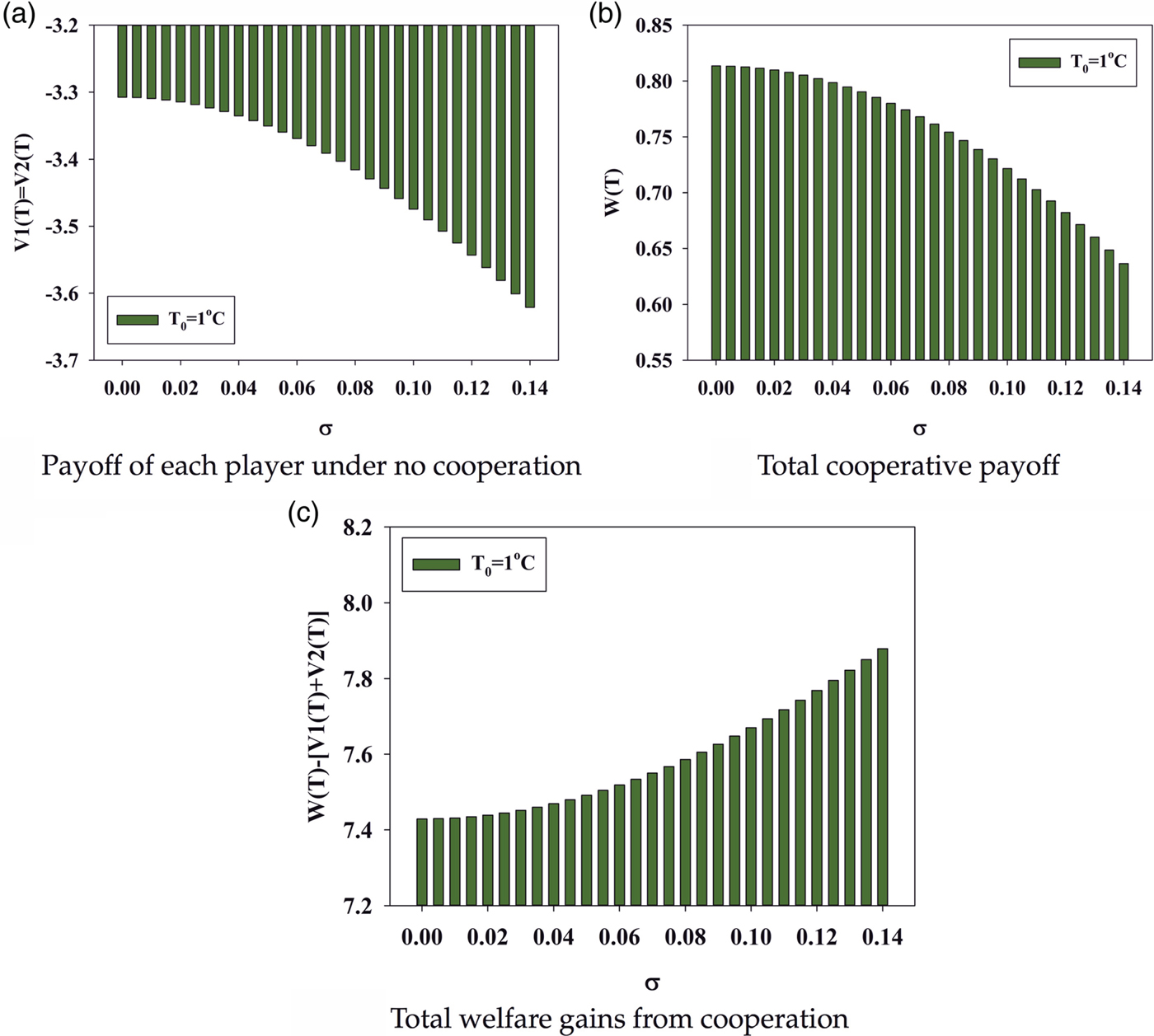
Figure 1. Effect of climate uncertainty in the case of symmetric players (T 0=1°C).
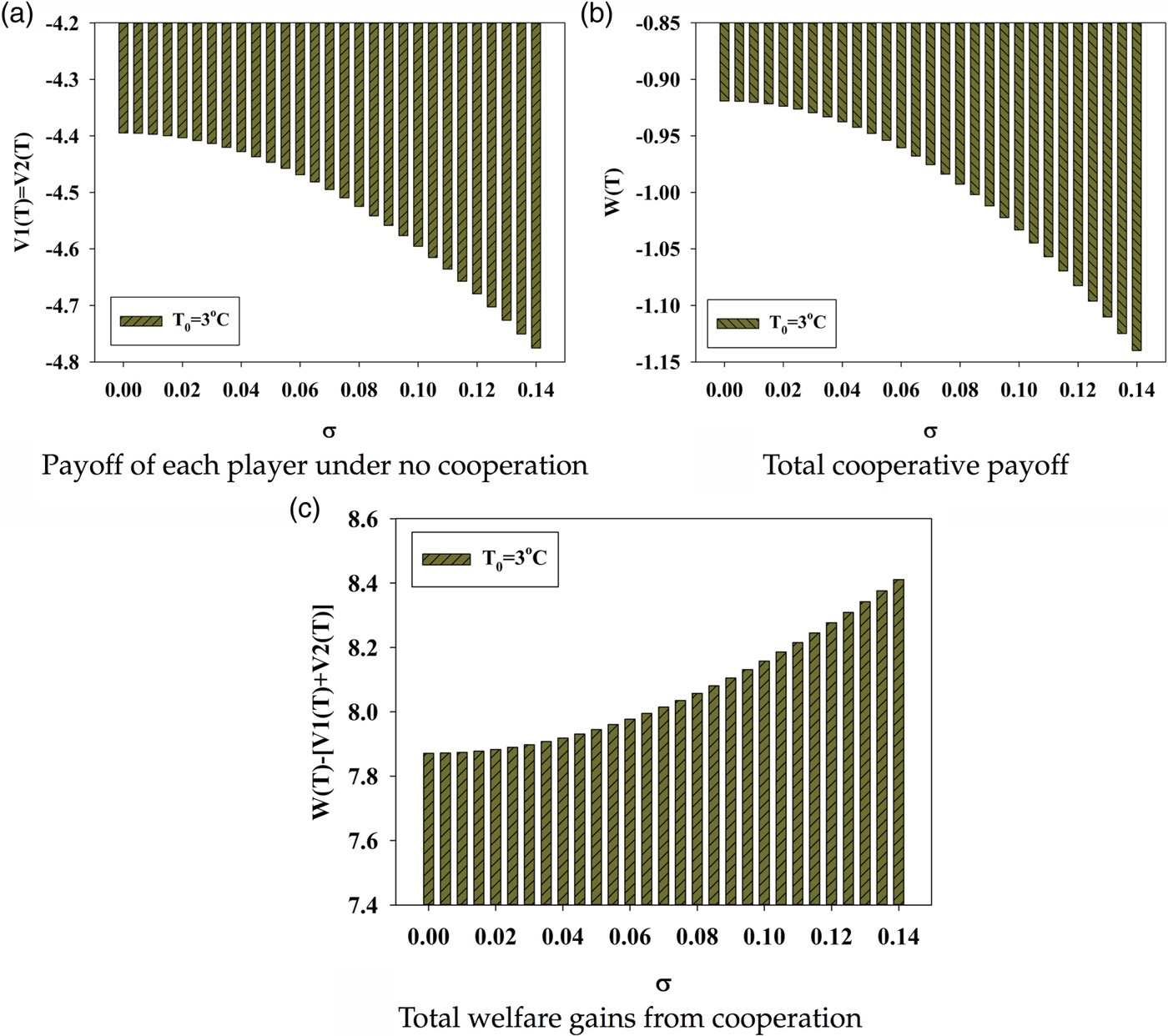
Figure 2. Effect of climate uncertainty in the case of symmetric players (T 0=3°C).

Figure 3. Effect of climate uncertainty in the case of asymmetric players (φ=0.5, γ=0).
It can be seen from figures 1 and 2 that players’ expected payoffs will decrease with higher climate uncertainty, whether or not they cooperate. Besides, it can be observed that the WGIC is an increasing function of parameter σ. These results are consistent with the theoretical predictions above for the symmetric case: even though the expected welfare of individual countries will be reduced by greater uncertainty about climate change in both the non-cooperative and cooperative cases, the (expected) WGIC is an increasing function of climate uncertainty. That is, the greater the climate uncertainty, the more important it is to have international cooperation.
From figure 3, one can see that the conclusions also hold for our particular case of asymmetric players where country 2 does not suffer from climate damages. It can be observed that, since player 2 does not suffer from climate damages, the uncertainty about climate change and initial temperature will not affect its expected payoff in the non-cooperative case, as illustrated by figure 3b. For country 1, its expected payoff in the non-cooperative case still decreases as climate uncertainty becomes larger. The total payoff under cooperation is also decreasing with uncertainty, as shown in figure 3c. However, the total welfare gain from cooperation is found to be an increasing function of climate uncertainty. These results are consistent with the theoretical predictions above.
Besides, based on equation (33), one can illustrate the effect of uncertainty on the instantaneous payoff transfers between countries. By setting τ=0 in equation (33), we focus on the initial payoff transfers, given the initial temperature T 0. As can be seen in figure 4, the transfers should go from country 1 to country 2 to ensure the stability of cooperation, given that country 2 does not suffer from climate damage. Also, the greater the uncertainty, the more country 1 needs (and is willing to) to transfer to country 2 to ensure cooperation.

Figure 4. Effect of climate uncertainty on the initial transfers between countries.
As mentioned above, the non-cooperative solutions for the more general asymmetric case (φ≠1 and γ≠{0, 1{) cannot be obtained analytically and would need the assistance of numerical methods. That is, given the model parameters, one can numerically solve the system of equations (9a)–(9f) to obtain the coefficients of players’ value functions with different values of climate uncertainty, and then investigate the effect of uncertainty and conduct comparisons with the cooperative solutions (see (16a)–(16c)).
Table 3 presents some numerical results to complement the analytical analysis above (where the asymmetric case is somewhat extreme). The bottom section in table 3 presents the results with larger climate uncertainty, compared with the top section. In each section, the parameter values of (φ, γ) reflect the asymmetry between the two players. It can be seen from table 3 that the total payoffs in the cooperative case (W) will decrease as the climate uncertainty becomes larger. The same will happen for the combined payoffs in the non-cooperative case (V 1+V 2). That is, climate uncertainty has a negative effect on the combined payoffs of players, whether or not they cooperate with each other. However, the welfare gain from cooperation (W−[V 1+V 2]) is always positive and increases as uncertainty becomes larger, which suggests that international cooperation is more important when facing greater climate uncertainty. Besides, the numerical results show that it is possible, in the case of asymmetric players, that the non-cooperative payoff of one player is reduced by larger climate uncertainty while the non-cooperative payoff of the other player is increased by larger uncertainty. For instance, with (φ, γ)=(1, 2), where the two players have identical benefits from emissions but player 2 faces larger climate damages, a larger climate uncertainty (a change in σ from 0.01 to 0.08) will reduce the non-cooperative payoff of player 2 (V 2) but increase that of player 1 (V 1). In this case, a larger climate uncertainty provides an incentive to the country with higher damage to implement relatively larger emission reductions (which also reduces its payoff) compared to the other country that, as a response, free rides by emitting more and thus increases its payoff. However, as stated above, the overall effect of increasing uncertainty is a reduction in the combined payoffs (V 1+V 2).
Table 3. Some more simulation results (r=0.04, a=1, ε=0.0047)

In addition, it can be seen from table 3 that the initial payoff transfer from player 2 to player 1 (F 1) varies as the asymmetry between players or the degree of climate uncertainty changes.Footnote 11 For instance, when the two players are fully symmetric, there is no need for a payment transfer between them. In contrast, with a very small γ, i.e., player 2 suffers much less from climate damage than player 1, the transfers to player 1 are negative, which implies the need for payment transfers from player 1 to player 2 to support the stability of cooperation. Also, the transfers needed to stabilize cooperation are larger when climate uncertainty is higher. With γ=2, when player 2 faces twice as much damage as does player 1, payment transfers from player 2 to player 1 are necessary to ensure stable cooperation, and the needed transfers are larger with higher climate uncertainty.
7. Concluding remarks and further research
This paper investigates the effect of climate uncertainty on international cooperation through a stochastic dynamic game in which the global temperature increase due to CO2 emissions is uncertain. It is shown that, even though greater climate uncertainty will reduce the expected welfare of players in both the non-cooperative and cooperative cases, it is always beneficial to cooperate with each other, and the expected welfare gain from international cooperation is larger with greater climate uncertainty. That is, the greater the uncertainty about global warming, the more important it is to have international cooperation on emission control. At the same time, more transfers will be needed to ensure stable cooperation among asymmetric players. These results suggest that the climate uncertainty can become another source of externality which lowers individual countries’ welfare. Since this kind of externality from ‘risk’ can also be free ridden by individual countries, the gain from cooperation will be larger if this externality (due to climate uncertainty) is larger.
Our results have important policy implications. In reality, individual countries become hesitant in climate cooperation and believe that they should not act or cooperate due to the uncertainty surrounding climate change. However, our results show cooperation can always benefit a country, provided there is an appropriate side payment mechanism. Moreover, the benefits from cooperation are larger when the climate uncertainty is higher, implying that it is more important to cooperate when we are more unsure about the future temperature increase. This suggests that with high climate uncertainty (due to the lack of scientific knowledge), we should make more efforts to help reach the international cooperation, which, of course, would require more side payment. However, as the climate research advances, which leads to less uncertainties regarding the evolution of global warming, the required size of side payment might be reduced.
This study is not without limitations. For instance, the analysis presented here is based on the game's analytical solutions, which can only be obtained for the case of unconstrained emissions (i.e., reversible emissions). The case of irreversible emissions (which can be more realistic), unfortunately, does not allow for an analytical solution and a comprehensive analysis for this case may need the assistance of advanced numerical methods. Therefore, we omit the discussion of irreversible emissions in our analysis. Further research should use numerical analysis to examine how uncertainty affects the benefits of international cooperation under the assumption of irreversible emissions.
Another possible extension is to include asymmetric uncertainty in the model. That is, the level of climate uncertainty can vary significantly in different countries or regions. More specifically, the temperature means as well as variances in the two countries or regions in the model can be different. Each regional temperature is affected by emissions from both regions, though the uncertainties governing the evolution of temperatures in the two regions may be different. This problem can be modeled as a stochastic dynamic game with two state variables, which can only be solved with the assistance of numerical methods.Footnote 12 Our numerical simulations show that, for two regions that differ in climate uncertainty only, one region will be worse off in its payoff (welfare) as its own climate uncertainty becomes larger, but better off as the other region's uncertainty becomes larger, in the absence of cooperation. The TWGIC cooperation increase with each region's climate uncertainty, though the total payoffs of the two regions under cooperation will be reduced by higher climate uncertainty in either region. Also, the size of the initial instantaneous payoff transfer (if any) to one region to ensure stable cooperation is negatively related to its own climate uncertainty but positively related to the other region's uncertainty. That is, in order to ensure cooperation, the countries/regions with higher uncertainty in climate need to compensate the ones with lower uncertainty. A more general and analytical analysis on the effect of asymmetric uncertainty in this context can also be a direction for further research.
Supplementary material
The supplementary material for this article can be found at https://doi.org/10.1017/S1355770X18000219.
Acknowledgements
The authors gratefully thank an Associate Editor and two anonymous referees for their helpful comments and suggestions on the preliminary draft of this paper, according to which the content was improved. We also would like to thank Jessica Coria, Thomas Sterner, Per Krusell, Knut Einar Rosendahl, Stefan Ambec, Carlos Chavez and Jesper Stage for their helpful discussions and comments on this paper. All errors and omissions remain the sole responsibility of the authors. The research leading to these results has received funding from the National Natural Science Foundation of China (No. 71603267), the European Union Seventh Framework Programme (FP7-2007-2013) under grant agreement (No. 266992), and the Swedish Foundation for Strategic Environmental Research for research funding via the research program Mistra Carbon Exit.


