1. INTRODUCTION
The cointegration framework of Engle and Granger (1987) is characterized by two widely held stylized
empirical facts. The first is that, of the set of economic time series
that exhibit trending behavior, many are adequately modeled by processes
that are integrated, usually of order one, I(1). The second is
that, despite this trending behavior, such series often tend to comove
over time according to a stationary, or I(0), process; that is,
they are cointegrated. Many empirical tests of important economic
hypotheses are carried out within the Engle and Granger framework, for
example, the relationship between long-run and short-run interest
rates—the term structure. The Engle and Granger approach has,
perhaps surprisingly, however, uncovered only very limited empirical
evidence in support of the term structure (see Campbell
and Shiller, 1987). An explanation often put forward for this is
that bond market series tend to be too volatile to be compatible with the
I(1)/I(0) framework. That is, the individual series
often appear visually to be more volatile, or less smooth, than would be
consistent with I(1) and when comovements between series are
analyzed (most simply by examining the spreads) these also tend to display
periods of volatility in excess of that typically associated with
stationary behavior. In the words of Campbell and Shiller, the spreads
tend to “move too much.”
One possible approach to dealing with the presence of extra volatility
is within the stochastic integration and cointegration framework
of Harris, McCabe, and Leybourne (2002). Here,
the restrictive stationarity requirement of first differences of
individual series and cointegrating error terms of the Engle and Granger
(1987) setup is replaced with a looser condition
that these are stochastically trendless; that is, they are simply
free of I(1) stochastic trends. This notion, of course,
encompasses the Engle and Granger setup as a special case. We outline this
framework in Section 2.
In Section 3 we turn to the issue of hypothesis testing in a
regression model representation. The central hypothesis of interest is
whether series are stochastically cointegrated (either stationary or
heteroskedastic), or not cointegrated. We suggest a residual-based
statistic to test the null of stochastic cointegration. Within stochastic
cointegration, we also consider the hypothesis that the cointegration is
stationary against the alternative that it is nonstationary
heteroskedastic, and we suggest a second statistic to test this. Moreover,
when applied to first differences of an individual series, this same
statistic can also be used to test the null of I(1) against
heteroskedastic integration. The asymptotic null distributions of these
two test statistics are derived under weak regularity conditions. Both are
shown to have normal limit distributions that, unlike most cointegration
tests, do not depend on the number of regressors involved. Their
consistency properties under associated alternative hypotheses are also
established.
Some Monte Carlo studies that examine the finite-sample size and power
characteristics of the new tests, along with those of their conventional
counterparts, are provided in Section 4. These highlight clearly the
benefits to be gained by adopting the new test procedures, together with
the shortcomings of using conventional ones, in the stochastic
cointegration framework. Finally, in Section 5 we apply our tests to bond
market data from several major economies. Our new testing framework
uncovers supporting evidence in favor of the term structure in the bond
market, in the same situation where conventional tests yield inconsistent
results. Notably, for all the interest rate series we consider here, we
conclude they are better modeled by heteroskedastically integrated, rather
than I(1), processes.
2. STOCHASTIC INTEGRATION AND
COINTEGRATION
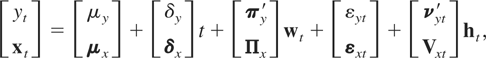
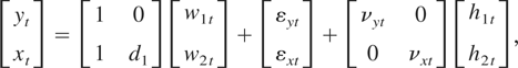
We first consider a variant of the model introduced in Harris et al.
(2002):
for t = 1,…,T. Here
zt, μ, δ, and,
εt are m × 1 vectors;
wt and ηt
are n × 1 vectors; ht and
υt are p × 1 vectors;
Π and Vt are m ×
n and m × p matrices, respectively. Only
the process zt is observed. The disturbances
εt, ηt,
υt, and Vt
are mean zero stationary processes, which may be correlated with one
another; wt and
ht are vectors of integrated processes. So,
apart from deterministics, zt consists of an
integrated component, Πwt,
together with a shock term, εt +
Vtht. This
latter term has a linear component, εt, and a
nonlinear component
Vtht that is
nonstationary heteroskedastic through its dependence on the I(1)
process ht. Note that it is entirely possible
throughout our analysis that wt and
ht contain identical processes, though we do
not enforce this restriction.1
In Harris et
al. (2002), ht =
wt. Here if any element of
wt is identical to that of
ht we would simply delete the corresponding
element of υt from Assumption
LP.
As regards the statistical properties of the disturbance terms in (1),
we make the following linear process assumption. This allows for general
forms of serial correlation, cross-correlation, and endogeneity.
Assumption LP. Let ζt =
[υt′,vec(Vt)′,
ηt′,
εt′]′ be generated by
the vector linear process
,
where
-
with C0 having full rank.2
- ξt is an independent and
identically distributed (i.i.d.) sequence.
- E(ξtξt′)
= I.
- For all i,
E(ξit16) is
bounded.
To examine the properties of the model more clearly, we make the
temporary simplifying assumption that μ = δ = 0.
Next, let ei be an m × 1
vector with 1 in its ith position and 0 elsewhere, so that
ei′zt =
zit, the ith element of the vector
zt. Then, from (1), we have
and if ei′Π ≠
0 then zit is said to
stochastically integrated. If, in addition,
ei′E(VtVt′)ei
> 0, zit is said to be
heteroskedastically integrated (HI) due to the term
ei′Vtht,
whereas if
ei′Vt = 0
then zit is simply I(1). So, a
stochastically integrated variable encompasses both ordinary and
heteroskedastic integration.
To model linear relationships between the variables in
zt, let c be a nonzero m
× 1 vector and consider
If c′Π = 0 then the variables of
zt are said to be stochastically
cointegrated. Under stochastic cointegration
c′zt =
c′(εt +
Vtht) behaves
like a stochastically integrated process net of its stochastic
trend component, and we refer to such a process as being
stochastically trendless.3
More
formally, a vector stochastic process, ut, is
said to be stochastically trendless if, as s → ∞
(t fixed),
where
is the sigma field of information of all the elements in the vector up to
time t. This implies that the mean square error optimal
s step ahead forecasts of a stochastically trendless process
converge to the unconditional mean of the process as the forecast horizon
s increases. Following the Beveridge and Nelson (1981) definition, such a process has no stochastic
trend (or permanent component), hence the terminology
“stochastically trendless.” An analogous definition has also
been used in the literature on economic convergence; see Bernard and
Durlauf (1996). Trendlessness is similar to the
concept of a mixingale and the associated notion of asymptotic
unpredictability, with the minor difference, in practical terms, that the
convergence of the conditional expectation in our definition is in
probability rather than in an Lp
norm.
This terminology is adopted because, under Assumption LP,
we can show that as
s → ∞ (with
t fixed)
In other words, the behavior of the process up to time t has
a negligible effect on its behavior into the infinite future.4
A proof of this result is available upon
request.
Therefore, even though the disturbances
υt have an infinitely persistent effect
on
ht+s, their effect on the
level of
Vt+sht+s
is only transitory. This implies that the product process
Vtht is
stochastically trendless, even if
Vt is
correlated with
υt. Although it is the
case that
Vtht
is nonstationary heteroskedastic, as it can be shown to exhibit a linear
trend in variance, it is the stochastically trendless nature of
c′
zt =
c′(
εt +
Vtht) that
bestows meaning to comovement of a nonstationary heteroskedastic kind.
When
c′E(VtVt′)c
= 0, then c′zt =
c′εt is stationary. If,
in addition, Vt = 0, the variables
are all integrated and cointegrated in the standard Engle and Granger
(1987) sense. Because of the stationary behavior
of c′zt in either case, we
simply refer to this as stationary cointegration. When
c′E(VtVt′)c
> 0, the variables zt are said to be
heteroskedastically cointegrated. Thus, stochastic cointegration
encompasses both stationary cointegration (possibly of the Engle and
Granger kind) and heteroskedastic cointegration.
To further position our concept of heteroskedastic cointegration, note
that I(1), HI, and the closely related stochastic unit
root processes all share the properties of having trends in their
variances although not being stochastic trendless.5
There is a growing body of evidence that many economic and
financial time series previously considered I(1) are more
appropriately modeled as HI or stochastic unit root processes.
See the results in Section 5 of this paper and, inter alia, Hansen (1992a), Leybourne, McCabe, and Tremayne (1996), Granger and Swanson (1997), Wu and Chen (1997),
and Psaradakis, Sola, and Spagnolo (2001).
When these models of nonstationarity
are extended to the multivariate cointegration setting, standard
cointegration implies that a certain linear combination of the series
becomes stochastically trendless
and any trend in variance is
removed. Hence, our definition of heteroskedastic cointegration
effectively provides a halfway point to standard cointegration, because
the linear combination becomes stochastically trendless, yet the trend in
variance remains.
3. HYPOTHESIS TESTS AND TEST
STATISTICS
Our primary goal is to determine if the system is stochastically
cointegrated. This null, and the alternative of noncointegration, may be
stated as H0 : c′Π =
0 and H1 : c′Π
≠ 0. Within stochastic cointegration, we may wish to know
whether stationary or heteroskedastic cointegration pertains. The null of
stationary cointegration against the heteroskedastic alternative may be
tested by partitioning H0 as
H00 :
c′E(VtVt′)c
= 0 and H10 :
c′E(VtVt′)c
> 0.
It proves convenient to interpret these hypotheses within a regression
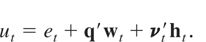
model. Partition zt into a scalar
yt and an (m − 1) × 1
vector xt as zt
=
[yt,xt′]′.
Then partitioning (1) conformably, and rearranging, we obtain
where yt, μy,
δy, and εyt are scalars,
xt, μx,
δx, and εxt are
(m − 1) × 1 vectors, and
πy′ and
νyt′ are 1 × n and 1
× p vectors, respectively, whereas
Πx and Vxt
are (m − 1) × n and (m − 1)
× p matrices. Letting c =
[1,−β′]′, α =
μy −
β′μx, κ =
δy −
β′δx,
et = εyt −
β′εxt =
c′εt, q′
= πy′ −
β′Πx =
c′Π, and
νt′ =
νyt′ −
β′Vxt =
c′Vt, then we have
Thus, the regression error term ut is
composed of the stationary term et, the
integrated term q′wt, and the
heteroskedastic component
νt′ht.
Note that ut need not have zero mean, so that
α is not an intercept in the usual sense. In the regression framework
we assume that there is only one cointegrating vector, so that
rank(Πx) = m − 1, which
imposes the restriction that n ≥ m − 1. This
implies that further subrelationships among the
xt variables in (3) are excluded.6
A special case of this model is studied by
Hansen (1992a). When q = 0 and
Vxt = 0, (3) corresponds to a
regression model when the regressors variables are all I(1) and
the error term is heteroskedastic, so that the regressand and regressors
are treated asymmetrically.
The null hypothesis of stochastic
cointegration against the alternative of noncointegration can now be
expressed via (3) as
H0 :
q =
0 and
H1 :
q ≠
0. Within
H0, the null hypothesis of stationary cointegration
against the heteroskedastic alternative is
H00 :
E(
νt′
νt)
= 0 against
H10 :
E(
νt′
νt)
> 0.
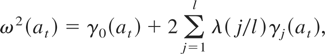
For later use, we also define the lag covariances for an arbitrary
process {at} by
and define a heteroskedasticity and autocorrelation consistent (HAC)
estimator of the long-run variance (LRV) by
where λ(.) is a window with lag truncation parameter l.
We also assume that Assumption KN, which follows, holds.
Assumption KN (Kernel and lag length).
- λ(0) = 1.
- 0 ≤ λ(x) ≤ 1 for 0 ≤ x < 1.
- λ(x) is continuous and of bounded variation on
[0,1].
- l → ∞ as T → ∞.
3.1. Testing H0 against
H1
To test stochastic cointegration against noncointegration we need to
test whether q = 0 in
Here, the null hypothesis is composite, encompassing both stationary
and heteroskedastic cointegration; whereas the alternative is
I(1) or heteroskedastic integration. Because of the level of
generality being entertained it is, however, not clear as to how to
construct an optimal test statistic with a tractable limit distribution
(even if we restrict ourselves to making Gaussian i.i.d. assumptions about
the distributions of the unobserved variables). These complications lead
us to examine instead a simple statistic for which we can at least
determine a limiting null distribution free of nuisance parameters and
also establish consistency. To this end, we consider
In the situation where all the disturbance terms are i.i.d.,
Snc with k = 1 would test for zero
autocorrelation in ut against the correlation
induced by the I(1) term
q′wt. When the disturbance
terms are not i.i.d., Snc needs to be
modified to eliminate nuisance parameter dependence resulting from
autocorrelation and also from the presence of
νt′ht.
This is accomplished by allowing k to increase with
T.7
The form of the statistic
Snc was earlier considered by Harris et al.
(2003) in the context of stationarity testing in
a deterministic regression.
Under the cointegrating null,
H0, the statistic
Snc
(when standardized with a HAC variance estimator) is asymptotically
N(0,1) and is consistent under the alternative of no
cointegration,
H1. This is the content of Theorem 1,
which follows. Because of the linear process representation, letting
k become large eliminates correlation between
ut and
ut−k under
H0, whereas the HAC variance estimator takes care of
the term
νt′
ht.
8 Cointegrating versions of KPSS stationarity
tests, such as that of Shin (1994), suffer from
the fact that it is not possible to remove the effects of nuisance
parameters in the partial sum process of ut
under the null of heteroskedastic cointegration, leading to incorrect
size. The simulation studies of Section 4 confirm this.
Under
H1, because of the presence of the
I(1) term
q′
wt, letting
k grow
does not eliminate correlation between
ut and
ut−k. This distinction is the
source of consistency of the test.
Because yt and
xt are observed, we estimate b =
[α,κ, β′]′ of (3) by means of
the estimator
given by
where Xt =
[1,t,xt′]′.
This estimator, described in Harris et al. (2002), is called an asymptotic instrumental variables
estimator (AIV). Under H0, a minor modification of the
proof of Harris et al. (2002) shows that
is consistent as k and T → ∞, in contrast to
the ordinary least squares (OLS) estimator, which is not consistent under
heteroskedastic cointegration unless xt
consists entirely of I(1) processes. We now construct (6) using
the AIV residuals:
We then have the following result.
THEOREM 1. Assume that the model (3), Assumption LP, and
Assumption KN hold. If k =
O(T1/2), l =
o(k), and l < k, then
(ii) under H1, the distribution
of
diverges as T → ∞.
Here
is defined in (8) using (7); ω2(.) is
defined in (5).
The first part of this theorem states that a properly standardized
statistic,
,
is asymptotically normal under stationary cointegration (which includes
Engle and Granger cointegration) and also under heteroskedastic
cointegration; the second part shows that the test is consistent under
H1. The same results arise if linear trends are
excluded from (3) and the fitted model.
3.2. Testing H00 against
H10
In decomposing the composite hypothesis H0 into
the null of stationary cointegration against the heteroskedastic
alternative, we need to test whether
E(νt′νt)
= 0 in (4), maintaining q = 0. Under the temporary
assumption that et,
νt, ηt,
and υt, are all jointly Gaussian i.i.d.
and uncorrelated with each other, it follows from a straightforward
application of McCabe and Leybourne (2000) that
a locally most powerful test of H00 against
H10 is given by
We then have the following result.
THEOREM 2. Under the conditions of Theorem 1,
(ii) under H10, the
distribution of
diverges as T → ∞.
Notice that
is calculated using
,
rather than simply
,
as (9) might suggest. This alteration is needed to center the statistic
and render it invariant to the variance of ut
under H00.
The structure of Shc can also be used to
test the null of I(1) against the alternative of HI for
any given individual series by simply constructing
by redefining
as
where
is an estimator of the trend coefficient δy given
by
.
We denote this statistic
.
It is a straightforward special case of our results to show that
if yt is I(1) and
diverges if yt is HI. The same
results arise if linear trends are excluded from (3), in which case
.
9 Analogous statistics can of course be
constructed for each element of the vector
xt.
4. SIMULATION RESULTS
In this section we investigate, via Monte Carlo simulation, the
finite-sample behavior of our new tests, comparing these with tests
applied assuming the conventional paradigm. To test for the null of
conventional cointegration we apply the Shin (1994) adaptation of the Kwiatkowski et al. (1992) (KPSS) stationarity test. This test uses an
efficient OLS estimator in which [T1/4]
([.] denoting the integer part) lead and lag terms in
Δxt are added into the regression
equation of yt on
xt; see Saikkonen (1991) for details. We denote this test
Kc. The tests
,
and Kc all require the use of a kernel and a
lag truncation parameter in their respective variance estimators. For all
tests we use the Bartlett kernel for λ(.). As regards choice of
l, we allow two schemes. The first simply fixes l =
[12(T/100)1/4], which is a fairly
mainstream choice in the literature, whereas the second is the automatic
data-dependent selection method of Newey and West (1994).
10 In the context
of stationarity testing, this has been demonstrated by Hobijn, Franses,
and Ooms (1998) to remove many of the
well-documented oversizing problems associated with KPSS tests.
Here we enforce the restriction that, for our new tests,
l <
k when
l is chosen automatically. Regarding the choice
of
k, we wish to avoid choosing
k in a data-dependent
manner as the
O(
T1/2) rate is designed to
deal with
all processes covered by Assumption LP. Of course,
O(
T1/2) is not uniquely defined, and so
different possibilities need to be considered. Here we examine three
candidates. These are
k =
[0.75
T1/2],
[
T1/2], and
[1.25
T1/2]. Although not exhaustive,
these choices nonetheless prove sufficient for us to gauge the
finite-sample influence of different values of
k and also for us
to recommend a value for use in practice.
The simulation model we examine is (2) with m = n =
p = 2. Specifically, our data-generating process is
and the stochastic processes of (10) are generated according to
with
(ε1t,ε2t,ε3t,ε4t,ε5t,ε6t,ε7t,ε8t)′
a multivariate standard normal white noise process. Here the
di, i = 1,2,3 are constants. Within
this setup, if d1 = d2 =
d3 = 0, then H00 is
true and stationary cointegration between two I(1) series
pertains, whereas if d1 ≠ 0, H1
is true and yt and
xt are not cointegrated in any sense
(irrespective of the status of d2 and
d3). If d1 = 0 with
d2 ≠ 0 and/or d3 ≠ 0,
there is heteroskedastic cointegration. This may exist either between two
HI series (d2 ≠ 0 and
d3 ≠ 0) or between an I(1) and HI
series (e.g., d2 = 0 and d3 ≠
0). The model is generated over t =
−99,…,0,1,…,T, with the first 100 startup
values discarded. We consider sample sizes of T = 200,400,600,
and the number of replications for all experiments is 10,000. Table
entries represent empirical rejection frequencies of the various tests,
based on regressions allowing constants but not trends, at the nominal
asymptotic 0.05 level (these being two-tailed tests in the case of
). For brevity, we only report results for the
tests applied to yt. In terms of notation in
the tables, if φi,j is not explicitly
given, its value is set to zero. Variants of the tests based on the
automatic lag selection are superscripted with an a.
In Table 1 we have d1 =
d2 = d3 = 0 throughout, so that
H00 is true—stationary cointegration
between two I(1) series. The
test has near nominal size, indicating that I(1) rather than
HI series are present, and any additional serial correlation in
the form of nonzero values of φε,y clearly
has little effect on its size. As regards the test
,
its size is well controlled apart from when
φε,y = 0.9 and
φε,y = φε,x
= 0.9. Here, when k =
[0.75T1/2] it is moderately oversized
and thus too frequently indicates absence of cointegration. However,
setting k = [T1/2] or
k = [1.25T1/2] virtually
removes the oversizing problems, especially if the automated variants are
considered. When we examine the test
,
we find that the choice of k has far less effect on the size.
For φε,y = 0.9 and
φε,y = φε,x
= 0.9, all three choices (whether based on automated variants or not)
produce oversized tests and thus indicate spurious heteroskedastic
cointegration, although the degree of oversizing is not particularly
serious and is mostly ameliorated as the sample size increases. On the
basis of these results then, specifically those pertaining to
,
we would conclude that setting k =
[0.75T1/2] is realistically too low to
maintain reliable finite-sample size. Notice that the nonautomated KPSS
cointegration test, Kc, is quite badly
oversized when φε,y = 0.9 and
φε,y = φε,x
= 0.9, and automating the lag choice struggles to correct this to a
satisfactory degree. Interestingly, the automated
Kc test can be badly oversized in the
presence of negative autocorrelation, unless the sample size is large.
None of the other tests, however, appear to be adversely affected by
negative autocorrelation.
Size of the tests under stationary cointegration:
d1 = d2 = d3 =
0
Table 2 examines the size and power of the
tests under six different models of heteroskedastic cointegration,
H10. In the first four, both
yt and xt are
HI (d2 ≠ 0 and d3 ≠
0); in the fifth yt is HI
(d2 ≠ 0) and xt is
I(1) (d3 = 0), with these roles being
reversed in the sixth model. The size issue relates to
,
and it is clear that the test does not appear particularly sensitive to
k, with size being controlled reasonably well for all choices,
across all model specifications. If anything, setting k =
[0.75T1/2] sometimes leads to slight
oversizing; setting k =
[1.25T1/2] occasionally yields slight
undersizing. When considering the power of
,
both fixed and automated variants exhibit consistency. The power does not
appear to change particularly dramatically across model specifications
either. Power does tend to decrease monotonically as k increases,
although the rate of decrease is fairly low. The test
is also seen to be consistent (aside obviously from when
yt is I(1)). The behavior of the
Kc test is much less predictable, however.
This is because, as mentioned in Section 3, the distribution of
Kc in the HI case depends on
nuisance parameters. This test can have very low or reasonably high power
to reject its null of stationary cointegration, depending on the nature of
the heteroskedastic cointegration. For example, if
xt is I(1) as in the fifth case, its
power is trivial. If, on the other hand, if
xt is HI and
νxt is persistent, as in the second or sixth case,
it can reject stationary cointegration very frequently. This differing
behavior is due to the inconsistency of the OLS estimator of β (= 1)
whenever xt is HI.
11 Busetti and Taylor (2003) demonstrate that the KPSS tests applied to an
individual series with heteroskedastic errors can overreject the null of
stationarity. In the current context, the cointegrating KPSS statistic
actually diverges because of the inconsistency of the ordinary least
squares estimator when xt is
HI.
Size/power of the tests under heteroskedastic
cointegration
In Table 3, we examine the power of the
tests under the case of no cointegration, H1, here
between two I(1) series (
is not included now). Consistency of
is clearly evident, as is the role of k in determining its
power. The power is seen to fall fairly rapidly with increasing k
for both fixed and automated variants.
12 These observations also apply to
,
though it has rather less power than
because it is not constructed to detect this alternative.
Notice
also that power of
often exceeds that of Kc. There is no
contradiction here, however: the optimality properties associated with the
raw form of the KPSS statistic, on which Kc
is based, do not necessarily carry over to the current empirical version
of the statistic, which needs to be robustified both to serial correlation
and to endogeneity. It is also apparent that the power of
Kc drops quite sharply when moving from the
fixed to automated lag selection.
Power of the tests under no cointegration
In unreported simulations, we also examined the properties of the
tests when some endogeneity is introduced. The first case revisited
H00, stationary cointegration between two
I(1) series, where we set
cor(ε1,ε5) = −0.7 and
cor(ε2,ε5) = 0.7, such that the increment
processes of εyt and
εxt are correlated with that of the random walk
w1t. The sizes of
were largely unaffected by introducing such correlation. A second case
revisited H10, heteroskedastic
cointegration between two HI series. Here we made
w1t and h1t
identical random walks, so that the I(1) process driving part of
the heteroskedasticity also drove the level of the processes. In addition,
we set cor(ε4,ε8) = 0.7, such that the
increment process of νxt was correlated with that
of the random walk h2t it multiplies into.
Again, the size of
remained reasonably accurate, and consistency of
(and
) appeared unaffected. Full details of these simulations are
available upon request.
All the preceding simulation results concerning
are pretty much in line with what we would expect given our theoretical
results of Section 3 regarding asymptotic normality of the tests, their
robustness to serial correlation and endogeneity, and their consistency.
They all detect the appropriate departures from their respective null
hypotheses. The choice of k remains an issue, however.
Predominantly led by the behavior of
,
the facts are that setting k too low can, in certain situations,
induce size distortions (cf. Table 1), whereas
setting k too high leads to a loss of power (cf. Table 3). Moreover, it seems rather unlikely that such
a trade-off can be entirely avoided however k is chosen. A
reasonable compromise would appear to be the middle value of the three we
have considered, and so we recommend setting k =
[T1/2] as a matter of practice. Whether
l is selected using a fixed or an automated method does not
appear particularly crucial to our test's performance, and we would
not favor one approach over the other.
Our results also highlight the problems of using OLS-based procedures
such as Kc to test for cointegration.
Inconsistency of the OLS estimator whenever the heteroskedastic
cointegration involves xt that is HI
causes the test to reject, so that Kc is
unable to discern between this situation (i.e., when series
“differ” by a heteroskedastic but stochastically trendless
term) and noncointegration (i.e., when series “differ” by a
stochastic trend term). Of course, we may take the view that because
neither situation represents a stationary cointegrating relation, a
rejection of the null of stationary cointegration is an appropriate
outcome. However, if the heteroskedastic cointegration involves
xt that is I(1), the same test tends
to no longer reject this null, which clearly cannot also represent an
appropriate outcome. This of course means that the inference drawn can
become crucially dependent on the ordering of the I(1) and
HI variables, even asymptotically. Such considerations do not
apply to our new tests as their asymptotic distributions are free of
nuisance parameters. It is also important to remember that when applying
,
we never actually need to distinguish between which series are
I(1) and HI. That is, we do not need to calculate the
test
for individual series. Perhaps the only rationale for calculating
is that it may provide early warning of situations where it would be
unwise to apply conventional cointegration tests.
5. AN EMPIRICAL EXAMPLE: THE TERM STRUCTURE
OF INTEREST RATES
A necessary empirical condition for the expectations theory of the
term structure of interest rates is that long-run and short-run interest
rates cointegrate. We test this empirically using monthly data from the
United States, Canada, the United Kingdom, and Japan, taken from the
OECD/MEI database. A single long-run interest rate,
Lt, and a variety of short-run rates,
Sit, are used for each country, and we
consider bivariate regressions of Lt on
Sit and also the reordered regression of
Sit on Lt.13
See the note to Table 4
for a full description of the data.
We calculate the same array of
statistics as in Section 4, where again the regressions include constants but
not trends. We also calculate the standard KPSS stationarity test allowing a
constant (denoted
Ks), to test individual series
for stationarity. Both fixed and automatic lag selection procedures are
employed for all tests, and, in view of the results of the previous
section, we set
k = [
T1/2].
The results are given in Table 4, where the
entries are p-values of the tests based on the asymptotic
distribution. Bold print indicates a p-value of 0.05 or less, and
in the current context we will consider this to represent a rejection of
the associated null hypothesis. As regards the individual series, we first
note that the KPSS test, Ks, indicates
rejection of I(0) for every one of the 17 individual interest
rate series considered. In addition, the
test shows that all of these interest rate series appears to be
HI rather than I(1), so that excess volatility would
certainly appear to be an issue for this data set.
14 It is easily shown that the KPSS stationarity test is
consistent when the alternative is HI.
Application to bond market data: p-values of
tests
Turning now to the bivariate regression results, first
Lt on Sit, we
see that according to
,
stochastic cointegration is not rejected for eight of the 13 pairs. In
both Canada and the United Kingdom, the nonrejection is unambiguous. In
the case of the United States the evidence is mixed; rejections are found
for two of the four pairs considered. No evidence of stochastic
cointegration at all is found for Japan, though the peculiar nature of
Japanese short-run interest rates in recent times (being effectively zero)
may partly explain this finding. According to the
test of the eight pairwise regressions that do not reject stochastic
cointegration, five represent stationary cointegration between HI
series (three for Canada, two for the United Kingdom) and three represent
heteroskedastic cointegration between HI series (two for the
United States, one for the United Kingdom). This pattern of results is the
same whether the lag selection is fixed or automated. When we consider the
regressions of Sit on
Lt, qualitatively, the results for Canada,
the United Kingdom, and Japan are unchanged. The United States now shows
no rejections of stochastic cointegration, with one of the four being
stationary cointegration, one being heteroskedastic cointegration, and two
being indeterminate. This makes the total of nonrejections now 10 out of
the 13 pairs. Thus, there is certainly a reasonable consensus of support
for the term structure of interest rates in these data, particularly if
the somewhat anomalous case of Japan is excluded from consideration.
A less coherent picture emerges if we examine the outcomes from the
OLS-based KPSS cointegration test, Kc. For
regressions of Lt on
Sit, conventional cointegration is rejected
for every one of the 13 pairs of long- and short-run rates if a fixed lag
selection is used (this drops to four rejections if lag selection is
automated, though as shown earlier the power of this test can be a good
deal lower than that of the fixed lag test). However, no rejections at all
are obtained for the reordered regressions of
Sit on Lt.
Hence, the differing degrees of excess volatility of long- and short-run
interest rate data appear to exert a substantial influence on the outcomes
for conventional OLS-based cointegration tests, to the extent that
inference can be crucially dependent on variable ordering. By way of a
contrast, the new procedures we have proposed in this paper are designed
to provide inference that is rather more robust when analyzing this sort
of data.
APPENDIX: Proofs
Notation and Conventions.
In what follows we assume that Assumptions LP and KN, the model (3),
and k = O(T1/2) hold. For the
model specified by equations (1)–(3), with
ζt =
[υt′,vec(Vt)′,
ηt′,
εt′]′, let
and define covariance matrices
.
Also define St to be the partial sum of the
ζt, that is,
ΔSt =
ζt. Selector matrices
Rυ, Rν,
Rη, and Rε are
defined implicitly such that υt =
Rυ′ζt,
νt =
Rν′ζt,
ηt =
Rη′ζt,
and εt =
Rε′ζt.
When taking expectations through an infinite summation sign, we generally
do not remark on the operation when obviously square summable linear
processes are involved.
For transparency, we analyze the regression model without a time trend
included, though all our results can be shown to extend to the trend case.
We also make repeated use of the following representations:
with
and where zk,t is defined
implicitly.
When dealing with LRV terms it is convenient to utilize the following
results. First, in manipulating expressions involving kernels we adopt the
notation λ+(j/l) =
2λ(j/l), j > 0, λ+(0)
= 1. Next, for any sequences {at} and
{bt} define
We use the convention that γj(a) =
γj(a,a). Then for the sequence
{at + bt} we
have
Also define for any sequences {at} and
{bt}
again with the convention that ω2(a) =
ω(a,a). So, we have for the sequence
{at + bt},
Thus, for δ > 0 we can write
Note too that
with the obvious modification for a = b.
In our applications at is often a product
sequence, at =
ct
ct−k, say. The summation in
s starts at k + j + 1 and in t starts
at t = k + 1. Then, (A.4) yields
Proof of Theorems.
We also use the following lemmas in establishing the results of
Theorems 1 and 2.
LEMMA 1. Under
where
Proof. In this case
.
Setting δ = 0, at =
et
et−k, and
bt =
zk,t we have that
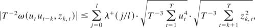
is bounded by (A.3). The first term in (A.3) is bounded by (A.5). That
is
where the order of the first right-hand side term is
O(l) (Assumption KN.2) and the second term is
Op(1), independent of k, by
Markov's inequality and Assumption LP. As for the third term,
recalling the expression for zk,t in
(A.2), note that
is Op(1) where
as follows from Harris et al. (2002). Thus, in
(A.2), the quadratic form in
is of a lower order than the two linear terms in
.
The linear terms are of the same order. So the two dominant terms in
are
.
But
and it is clear that the second dominant term is of the same order.
So,
.
Hence
The same method of proof shows that
|ω(zk,t,et
et−k)| and
ω2(zk,t) are also
Op(lT−1/2).
Thus,
Applying Theorem LRV of Harris, McCabe, and Leybourne (2003) (with n = 1, α = 2, and
μ = 0) then shows that
.
█
LEMMA 2. Under
.
Proof. Now
.
Setting δ = 2, at =
utut−k,
and bt =
zk,t we have that
is bounded by (A.3). The first term in (A.3) is bounded by (A.5). That
is,
where the first right-hand side term is O(l) and the
second Op(1). The dominant term of
is
where the first two Op(1) results can be
shown to hold via a simple modification of the approach of Harris et al.
(2002). Thus
and so
|T−2ω(utut−k,zk,t)|
is bounded by an
Op(lT−1/2)
variable. That
|T−2ω(zk,t,utut−k)|
and
T−2ω2(zk,t)
are also bounded by an
Op(lT−1/2)
variable follows similarly. Combining these results gives
Because et is of a lower order of
magnitude than
νt′ht
it follows by similar arguments that
LEMMA 3. Under
where
with B1 a Brownian motion
process.
Proof. Write
The key to the proof lies in replacing
vec(ζtζt−k′)vec(ζt−jζt−k−j′)′
in (A.6) by E
{vec(ζtζt−j′)}E
{vec(ζtζt−j′)}′
in (A.7). This means that the convergence in square brackets is
nonstochastic and thus the continuous mapping theorem (CMT) is sufficient
to deduce the asymptotic distribution. Also the quantity in square
brackets converges to Ω22 because it can be shown
to be a consistent estimate of the long-run variance of
vec(ζtζt−k′),
which is the definition of Ω22, that is,
.
Then ΩPP =
(Rν [otimes ]
Rν)′Ω22(Rν
[otimes ] Rν) by definition.
The validity of replacing
vec(ζtζt−k′)vec(ζt−jζt−k−j′)′
by the double expectation involves establishing the following sequence of
results (expressed in the scalar case for simplicity). That is,
The complete proofs of these steps are available from the authors on
request. Notice that the last equality shows the virtue of using the
expectation device as the CMT and then delivers the result in a very
straightforward way. █
LEMMA 4. Under
where
and σe2 =
E(et2).
The proof is similar to that of Lemma 1 and is thus omitted.
LEMMA 5. Let ζt satisfy
Assumption LP and let k =
O(T1/2). Then, as T →
∞,
where W =
Rυ′B1
and P = (Rν [otimes ]
Rν)′B2
where B1 and B2
are independent Brownian motion processes.
Proof. First rewrite using
ΔSt =
ζt, so that
The proof proceeds by applying the Beveridge–Nelson
decomposition to the first term and showing that the second term is
asymptotically negligible. We use the notation
where
and the coefficients are defined by
Apply Theorem BN of Harris et al. (2003) to
vec(ζtζt−k′)
to get a martingale approximation,
mk,t, a remainder term
rk,t, and an overdifferenced factor
.
The idea is that the martingale term is dominant and that the dependence
on k is absorbed into its variance. In this way the proof of
convergence to a stochastic integral can be treated by conventional
methods of analysis. Thus,
We find
The first result follows directly from Theorem SI of Harris et al.
(2003), and the second is established along very
similar lines. The last follows by writing
where at =
νt−kνt′υt.
The first term can be shown to disappear on exploiting the properties of
the increment process, that is, that
Et−k{at
−
Et−k(at)}
= 0; the second term disappears by applying Theorem 3.3 of Hansen
(1992b).
Thus,
Now, because k = o(T), it follows from
Theorem FCLT of Harris et al. (2003) that
jointly with
where MT,[Ts] =
T−1/2
[sum ][Ts]mk,t.
Thus Theorem SI of Harris et al. (2003) applies,
and setting BQ ≡
(Rν [otimes ]
Rν)′B2 =
P and U ≡
Rυ′B1 [otimes ]
Rυ′B1 =
W [otimes ] W we have that
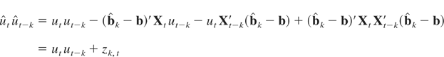
Proof of Theorem 1.
Part (i) (Null distribution). Sections (a) and (b) derive the
asymptotic null distribution of
under H00 and
H10, respectively.
(a) Under H00,
ut = et and from
Harris et al. (2002),
,
Op(T−1)]
and
are all Op(1). Consequently, using (A.2)
we find
Because et =
c′εt is a linear
combination of a vector linear process, it follows from an application of
Theorem FCLT of Harris et al. (2003) that
where by Lemma 1,
.
Thus,
(b) Under H10,
ut = et +
νt′ht,
and from a minor modification to the results of Harris et al. (2002),
are Op(1). Hence, using (A.2) we find
Now, substituting ut =
et +
νt′ht,
we can write
where W =
Rυ′B1 and
P = (Rν [otimes ]
Rν)′B2 and
B1 and B2 are independent Brownian
motions with covariance matrices Ω11 and
Ω22. The weak convergence follows from Lemma 5.
The covariance matrix of P is
ΩPP = (Rν
[otimes ]
Rν)′Ω22(Rν
[otimes ] Rν).
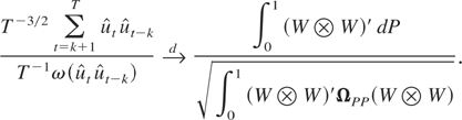
Combining the results of Lemmas 2 and 3 shows that
We now require the distribution of the ratio of
.
As shown in Lemma 5,
Next the CMT, with the preceding vector as argument and the ratio as
the map, applies to conclude that
As
conditional on W, the distribution in (A.8) is
unconditionally N(0,1).
Part (ii) (Consistency). Under H1,
ut = et +
q′wt +
νt′ht
where q ≠ 0. Here, it is easy to show that
,
and, using (A.2), this implies that
is of the same order in probability as
utut−k.
It is then straightforward to deduce that
Now we require a bound for the order of probability of
,
which again is the same as the order of probability of
ω2(utut−k).
Setting a = b =
utut−k
and δ = 2 in (A.5) yields
Thus we conclude that
at most. Hence the distribution of
diverges at least as fast as
.
█
Proof of Theorem 2.
Part (i) (Null distribution). Under
H00, ut =
et we have
.
Then, it follows from (A.1) that
where σe2 =
E(et2). Write
Here FT(s) is the partial sum
process of {et2 −
σe2} that weakly converges to
F(s) by Theorem 3.8 of Phillips and Solo (1992). Then, noting by integration by parts that
,
we can use the CMT to deduce
where F(s) is a Brownian motion with variance
ωe22, as defined in Lemma 4. Hence,
is normally distributed with mean zero and variance
which shows
From Lemma 4,
,
and so the result follows.
Part (ii) (Consistency). Under
H10, ut =
et +
νt′ht
we have
.
We may write
From (A.1),
is of the same order in probability as ut,
and it is then straightforward to show that
and hence
In the denominator,
(where
)
are of the same order in probability. Setting a = b =
ut2 −
σu2 and δ = 2 in (A.4)
yields
It is easily shown that both
are Op(1). Hence
ω2(ut2 −
σu2) and consequently
are Op(lT2) at most. So,
the distribution of
diverges at least as fast as
.
█