1. INTRODUCTION AND MOTIVATION
The p-dimensional cointegrated vector autoregressive (VAR)
model for I(2) variables, without deterministic terms and just two lags,
is given by the error correction model
where the εt are independent and identically
distributed (i.i.d.) (0,Ω). The freely varying parameters are
As usual, α⊥ denotes an orthogonal complement of
α, and we define the p × r matrix β =
τρ. Notice that the column dimension r of β is
between 0 and p and the same holds for the row dimension
r + s of ρ. Hence, s < p
− r. In the analysis of the I(2) model it will be important
to specify r and s such that r =
rk(αβ′) and s = rk(τρ⊥).
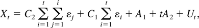
Under suitable conditions on the parameters (see Johansen, 1997), the equations in (1) have a solution
of the form
where Ut is stationary and the
coefficient matrices satisfy the relations
so that the processes Δ2Xt
= C2εt +
C1 Δεt +
Δ2Ut and
τ′ΔXt =
τ′C1εt +
τ′ΔUt are stationary. Thus the
solution is an I(2) process, and there are r + s
cointegrating relations given by the I(1) process
τ′Xt. The model also allows for
multicointegration (see Engle and Yoo, 1991),
that is, cointegration between the levels and the differences because
β′Xt +
ψ′ΔXt =
β′Ut +
ψ′C1εt +
ψ′ΔUt is stationary.
Equivalently one can show, because
τ′ΔXt is stationary, that
β′Xt +
δτ⊥′ΔXt
is stationary, where δ =
ψ′τ⊥(τ⊥′τ⊥)−1
is the so-called multicointegration parameter.
The theory of the I(2) model is developed by Boswijk (2000), Johansen (1997, 2005), Kongsted (2005),
Paruolo (1996), Paruolo and Rahbek (1999), and Rahbek, Kongsted, and Jørgensen
(1999).
It has been shown that the likelihood ratio test for the ranks
r and s has an asymptotic distribution that can be
expressed in terms of Brownian motions and integrated Brownian motions and
that has to be tabulated by simulation. Moreover, the asymptotic
distribution of the maximum likelihood estimator of the cointegrating
parameters τ, ρ, and β is quite involved, as it is not mixed
Gaussian. However, many hypotheses on these parameters can be tested using
asymptotic χ2 tests (see Boswijk,
2000; Johansen, 2005). We give
subsequently an example of such hypotheses that can be formulated and
tested in the I(2) model.
2. AN EXAMPLE OF HYPOTHESES ALLOWING FOR
ASYMPTOTIC χ2 TESTS
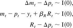
Denote by mt the log nominal money stock,
by pt the log price level, by
yt log real income, and by
Rt a long-term interest rate and define
Xt =
(mt,pt,yt,Rt)′.
Suppose mt ∼ I(2),
pt ∼ I(2),
yt ∼ I(1), and
Rt ∼ I(1). Moreover consider the
following cointegration relations:
- mt −
pt ∼ I(1) (i.e., log real money is
I(1))
- mt −
pt − yt +
βR Rt ∼ I(0)
(i.e., there exists a stationary money demand relation with unit income
elasticity)
- Rt −
Δpt ∼ I(0) (i.e., the “Fisher
effect” holds, meaning that the real interest rate is
stationary)
The unit root and cointegration properties of the variables are in
line with those found in Lütkepohl and Wolters (2003) for a system of German quarterly data except for
some of the values assumed for the cointegration parameters. Therefore one
may wish to formulate these hypotheses in the cointegrated model for I(2)
variables and develop the likelihood ratio test to check whether the
structure is compatible with the data.
We want to show that the hypotheses discussed earlier can be
formulated as hypotheses on the parameters ρ, τ, and ψ that
have the property that likelihood ratio tests of the restrictions are
asymptotically χ2.
Under the assumption that the process Xt
is I(2) it holds that
ρ′τ′Xt−1 +
δτ⊥′ΔXt−1
and τ′ΔXt are I(0). Therefore
we want to express the preceding relations in terms of the parameters
τ, β = τρ, ψ, and δ =
ψ′τ⊥(τ⊥′τ⊥)−1.
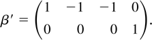
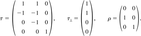
For our system p = 4, and from the cointegrating relations
we find that τ is 4 × 3, so that r + s =
3. We see that there are two relations that involve levels, so that
r = 2, and β has dimension 4 × 2 and is given by
This shows that the hypotheses formulated previously imply that
Hence the relations fully specify the matrices τ, ρ, and β
= τρ in this case. We denote the specific τ, ρ, and β
matrices by τ0, ρ0, and β0,
respectively. With this notation the model reduces to
and we next find the implications of the assumptions for the 4 ×
2 parameter ψ.
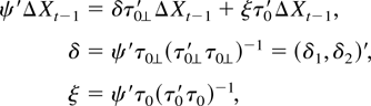
Because
τ0′ΔXt−1 is
stationary we decompose
ψ′ΔXt−1 as
where we used that δ is 2 × 1 and that
τ0(τ0′τ0)−1τ0′
+
τ0⊥(τ0⊥′τ0⊥)−1τ0⊥′
is equal to the identity matrix. Hence we can rewrite the equations in (1)
as
Notice that the coefficients δ are identified by the choice of
β = β0 and τ⊥ =
τ0⊥ and that
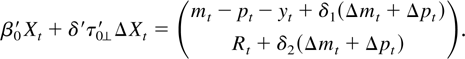
Now consider the stationary (multicointegrating) relation
By a linear transformation of the rows, which can be absorbed in
α, we can eliminate
δ1(Δmt +
Δpt) from the first equation and find
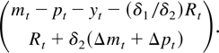
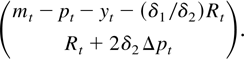
that the model implies stationarity of the linear combinations
Because Δmt +
Δpt =
2Δpt +
Δmt −
Δpt and
Δmt −
Δpt is stationary, we have that the
model, with τ0 and β0 as given before,
allows the stationary relations
Hence we see that we can define βR =
−δ1 /δ2, and the only extra
restriction we need to test is the hypothesis δ2 =
−0.5. Thus the restrictions formulated previously can be tested
successively as the hypotheses
The first hypothesis is a test on cointegrating ranks, and the
asymptotic distribution is nonstandard and tabulated by simulation (see
Johansen, 1997). It follows from the results in
the same paper (see also Boswijk, 2000; Johansen, 2005) that
are asymptotically distributed as χ2(4) and
χ2(1), respectively. In general one cannot expect
hypotheses on the coefficient δ to give asymptotic χ2
tests (see Paruolo, 2000), but
specifies τ⊥ completely, and when that is the case,
one can in fact show that a test on δ, and hence
,
is asymptotically distributed as χ2(1).
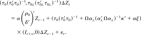
This can be seen by the “nominal-to-real” transformation
(see Kongsted, 2005),
which satisfies a model of the form
Premultiplying with
(τ0,τ0⊥)′ gives the I(1)
cointegration model
with parameters
and
.
Thus the transformed model is an I(1) model with linear restrictions on
partly known. A hypothesis on δ is therefore a hypothesis on
in an I(1) model, which is known to give asymptotic χ2
tests (see Johansen, 1991).