2. THE MODEL AND TEST STATISTICS

The basic model is an m-dimensional VAR model. Using conventional notation, the model can be described as

where z_t is an m × 1 vector of time series, z_t−1,…z_t−p, are 1 up to p lags of z_t, ε_t are i.i.d. random variates following multivariate N(0,Σ) with Σ being positive definite, A₁,…,A_p are conformable parameter matrices, and μ is an m × 1 vector of parameters. The error correction form of (1) is

with

The hypothesis of cointegration in the vector process z_t can be formulated as testing the rank of the Π matrix (Johansen, 1988, 1991). When the null hypothesis is that the cointegrating rank is r, the trace test statistic (λ_tr) is given by

where r is the cointegrating rank order and λ_i is the ith largest eigenvalue related to the Π matrix. The sequential tests start from the null hypothesis r = 0 (namely, all eigenvalues are 0's). If this hypothesis is rejected, one continues to test r ≤ 1 and stops testing the first time the hypothesis is not rejected or after r ≤ m − 1. For 0 < r < m, z_t is a cointegrated process; otherwise, it is nonstationary if r = 0 (or stationary if r = m). The asymptotic distributions of the trace statistic are affected by the assumption on the time trend in the process. If the constant in (2) is restricted to the cointegration space, the process contains a stochastic trend. If it is unrestricted, then the process contains both a linear time trend and a stochastic trend. Although other assumptions on the time trend have also been considered (Johansen, 1996), these two are used most often in applied studies.

The small sample correction for the preceding test statistic proposed by Johansen (2000, 2002) is of Bartlett type. The idea is to approximate the expectation of the likelihood ratio test statistic and to thereby correct it to have the same mean as the asymptotic distribution. The correction factor depends on moments of functions of the random walk and functions of the parameters. The exact formulas and coefficients necessary to compute the factor can be found in Johansen (2002).

We examine the performance of two widely used IC in the simulations: AIC (Akaike, 1973) and SC (Schwarz, 1978).²

where

is the maximum likelihood estimate of the variance-covariance Σ of the innovation (ε_t's) and K is the number of free parameters in the model, which, other things being equal, increases with the lag order (p) and the cointegrating rank (r) assumed in the model. The first term in equations (4) and (5) is the log determinant of

, which measures lack of fit of the model. The second term penalizes overparameterization of the model. It is clear from (4) and (5) that SC punishes model overparameterization more than AIC for sample sizes equal to or larger than eight.

Clearly, the IC method and the trace test are closely related. They both condition on the feature of matrix Π. The trace test detects the rank of Π by testing the statistical significance of the eigenvalues related to Π. The IC method determines cointegrating rank by balancing the benefit and cost of adding additional restriction vectors (cointegrating vectors) to the model. Specifically, if Π has rank r, it may be written as the product of two matrices: Π = αβ′, where α and β are of dimension m × r. We may regard β′z_t−1 as r linear restrictions/combinations on right-hand-side variables z_t−1. If a restriction is true, it must carry some useful information to explain the variation in the left-hand-side variables z_t. The more significant the restriction is (correspondingly, the larger the associated eigenvalues of Π), the more information it can convey. If the restriction is true, the useful information it contains should be enough to offset its cost (introducing more parameters to the model). IC would accept the restriction in this case. If, on the other hand, the restriction is insignificant or false, the information it carries cannot offset the cost; IC would reject the addition of such a restriction.

3. MONTE CARLO SIMULATION I

In this section, we investigate the sampling properties of AIC, SC, and two forms of the trace test in determining the cointegrating rank of model (1) assuming the lag order is known. To this end, Toda (1994, 1995) shows that, without loss of generality, we can study a “canonical form” model.³

where the dimensions of w_t, w_1,t, and w_2,t are m, r, and (m − r), respectively, δ is a nonnegative scalar, e_m−r = (0,…,0,1)′ is an (m − r)-dimensional vector, all eigenvalues of Ψ lie inside the unit circle, and finally,

Clearly, the subvector process w_1,t is stationary and w_2,t is nonstationary. They are correlated by a matrix Θ. The process w_2,t also contains a linear deterministic trend unless δ = 0. Following Toda (1995), we consider a bivariate VAR(1). There are three possibilities in regard to the cointegration relations of DGP (6).

First, if r = 0, that is, (6) contains only nonstationary components, then model (6) simplifies to

and ε_t ∼ i.i.d. N(0,I₂). In (7), the only parameter is δ.

Second, if r = 1, (6) becomes a cointegrated process with the following explicit form:

where |ψ| < 1 and |θ| < 1.

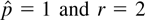
Third, if r = 2, (6) becomes a stationary process

where ε_t ∼ i.i.d. N(0,I₂) and Ψ is further assumed to be diagonal

where |ψ_a| < 1 and |ψ_b| < 1.

In this and the next simulation, we examine the IC performance for four sample sizes: 30, 50, 100, and 200. The number of replications for each sample size is 5,000. Following tradition, for each replication we generate an additional 50 random observations to eliminate start-up effects. Toda (1995) explicitly considers the impact of starting values of w_t on the test performance. It is clear from his reported results that the relative performance of the trace test does not change significantly for three different sets of starting values. To save space, and also to follow tradition, we only report the simulation results using w₀ = 0 in all cases.

The results reported in Table 1 are based on DGP (7), a nonstationary process without cointegration relations (r = 0). Each entry is the percentage of times the four test procedures, AIC, SC, trace test (λ_tr), and the small sample adjusted trace test (λ_tr*) of Johansen (2002), correctly determine the cointegrating rank of the simulated data.⁴

Performance of IC and trace tests for cointegrating rank: r = 0, Simulation I

The performance of SC improves considerably when the sample size increases. For example, when T = 50, the frequencies with which it correctly identifies the rank are 93.2%, 82.8% and 86.4% when δ = 0.0, 0.2, and 1.0, respectively. At T = 100, the success ratios of SC are all larger than 90% for the different values of δ. When the sample size further increases to 200, SC almost always finds the correct rank (99.5%) in the case of δ = 0. In models with a linear trend, the percentages are also high, 97.3% or higher. In contrast, the change in sample size has little impact on AIC, which confirms that SC is consistent whereas AIC is not.

Using DGP (8), we examine the performance of the four procedures when the true model is a bivariate cointegrated process with r = 1. We use following parameter values in the simulations: δ = 0.0, 0.2, and 1.0, ψ = 0.8 and 0.9, and θ = 0.0, 0.4, and 0.8 (results based on negative θ are omitted because they are very close to their positive counterparts). Table 2 contains the simulation results for two small sample sizes, T = 30 and 50. Clearly, all four procedures perform poorly in small sample sizes. In models with θ = 0.0 and δ = 0.0, namely, no correlation between the stationary and nonstationary components and no linear trend, λ_tr makes the correct rank choice only 7.8% of the time (the small sample correction actually leads to slightly worse performance, 6.6%). The success ratio of SC is higher but still low (14.4%). AIC performs best in this case. When the two component series are more closely related (larger θ), the performance of all procedures improves. The frequencies that SC and λ_tr find correct rank, when θ = 0.8, increase to 36.6% and 27.4%, respectively. The presence of a linear trend in the data appears to have different impacts for IC and the trace tests. Compared to the results when δ = 0.0, the performance of SC when δ = 1.0 improves considerably (29.4% vs. 14.4%), whereas AIC's performance also increases to 63.0%. The numbers remain small for both λ_tr and λ_tr* (9.0% and 8.4%). As in the model with δ = 0.0, the test power increases for larger correlation (θ = 0.8 and δ = 1.0). And SC (54.2%) still leads the trace tests (24.8%).

Performance of IC and trace tests for cointegrating rank: r = 1, T = 30, 50, Simulation I

The second part of Table 2 repeats the preceding simulations with the autoregressive coefficient further approaching 1 (ψ = 0.9). Not surprisingly, all four test procedures are less powerful, as the stationary component is now closer to a nonstationary component. In the case of δ = 1 and θ = 0.8 (the rightmost column), SC concludes with zero or two unit roots 70.0% (100% − 30.0%) of the time, even if the true model has only one unit root, whereas the trace test is more likely to err (about 90%). Correcting for small sample bias does not help.

The results in the third and fourth sections of Table 2 are based on the slightly larger sample size of 50. In general, all procedures, especially SC, λ_tr, and λ_tr*, perform better when ψ = 0.8 in the DGP. The improvement is obvious for θ = 0.8. The procedures λ_tr and λ_tr* now have similar power as SC in models without linear trends. Nevertheless, at this sample size, AIC and SC are still better choices than are the trace tests when a linear trend is present (δ > 0). Comparing the results in the fourth section with the second section, we find that the increase of T from 30 to 50 does not lead to much improvement on performance for any of the four tests if ψ = 0.9 with the exception of θ = 0.8.

Results in Table 3 are also based on DGP (8) using a moderate sample size of 100 and a larger size of 200. When T = 100, both λ_tr and λ_tr* outperform SC in the model with δ = 0.0 but are outperformed by the latter if δ ≠ 0.0. Although the performance of AIC is primarily affected by δ, the correlation coefficient θ is an important factor in determining the performance of SC, λ_tr, and λ_tr*, given ψ. For example, when θ = 0.0 or 0.4, and ψ = 0.8, all procedures perform poorly, even when the sample size is 100. In contrast, all perform quite well when the two innovations are strongly correlated. The low power of the test procedures against large ψ is still evident when T = 200. If ψ = 0.8, all four procedures perform well, except AIC in the models with δ = 0. When ψ = 0.9, the performance of SC, λ_tr, and λ_tr* deteriorates significantly (lower than 60%) in models with low correlations. These three procedures perform equally well (around 90%) when θ = 0.8; in other cases, λ_tr and λ_tr* outperform SC. Notice in the fourth section of the table (ψ = 0.9) that the power of SC is extremely low when δ = 0.0 and θ is small, even at the sample size of 200 (9.2% and 17.6% for θ = 0.0 and 0.4, respectively). In additional simulations we conducted (not reported in detail here), only when the sample size increases to 400 does the ratio increase to 52% and 76.1%. These percentages increase to 79.1% and 93.4% when T = 500.

Performance of IC and trace tests for cointegrating rank: r = 1, T = 100, 200, Simulation I

Table 4 contains simulation results assuming the DGP is a stationary process (equation (9)). The parameters that affect the distribution of the test statistics in this model are the two autoregressive coefficients, for which we use ψ_a = 0.5, 0.7, and 0.9 and ψ_b = 0.7, 0.8, and 0.9. In small samples, AIC performs much better than SC, λ_tr, and λ_tr*. SC outperforms λ_tr and λ_tr* when T = 30 but does not outperform them when T = 100. The later three procedures perform similarly when T = 50. As before, the power of the procedures decreases as the series considered approach nonstationary processes (ψ_a and/or ψ_b approaches 1). For example, there is a high probability (about 70%) that SC, λ_tr, and λ_tr* conclude that the DGP (9) is nonstationary, without cointegration relations, when T = 50 and ψ_a = ψ_b = 0.9 (not reported in the table). Finally, if T increases to 200, all procedures work well even for ψ_a = ψ_b = 0.9 (the lowest score is SC's 83.9%).

Performance of IC and trace tests for cointegrating rank: r = 2, Simulation I

We end the discussion of the first simulation by noting that the trace test tends to perform quite well for the cases where the DGP is of full rank (r = 2). This is not surprising, as Johansen (1992) has shown analytically that the probability of overestimation of rank does not go to zero if a fixed significance level is used in the sequential trace tests. However, in the full rank DGP (r = m), it is impossible to have overestimation in the trace test, which helps explain the good performance of the trace tests in this model. Similarly, as mentioned in the Introduction, AIC is also inconsistent and overestimates the cointegrating rank. This explains why AIC does quite well for models with r = 2 although performing poorly in other cases.⁵

4. MONTE CARLO SIMULATION II

As discussed in the Introduction, both the lag order determination and the test of cointegration relations in a multivariate model relate to model specification. In the preceding simulations, we have assumed that the lag order of the DGP is known, which is rarely true in empirical studies. When the lag order is unknown, the practice is to determine the lag order first using either IC or sequential likelihood ratio tests. In the second stage, a parametric test such as λ_tr is used to determine the cointegrating rank conditional on the lag order chosen in the first stage. In this section, we examine the performance of AIC and SC when they are used to determine the lag order and the cointegrating rank simultaneously. For the purpose of comparison, we also implement the two-step procedure to the new DGP. The new DGP again includes two series: y_t and x_t. Specifically, the DGP is described by the following equations:

Many researchers have used DGPs similar to (10). A short list includes Banerjee, Dolado, Hendry, and Smith (1986), Engle and Granger (1987), Blangiewicz and Charemza (1990), Hansen and Phillips (1990), Gonzalo (1994), and Haug (1996). To examine the impact of the model parameters on the test performance, we use the following values in the experiments: a₁ = (0, 1), ρ = (0.1, 0.3, 0.5, 0.7, 0.85, 0.9, 0.95, 1), θ = (−0.8, −0.5, −0.25, −0.1, 0.0, 0.1, 0.25, 0.5, 0.8), and η = (−0.8, −0.5, −0.25, −0.1, 0.0, 0.1, 0.25, 0.5, 0.8). Because, unlike other cointegrating rank tests, both the IC and trace tests do not depend on the standard deviation of the second innovation process φ_t, σ, we fix it at σ = 1. Nor, in the case of equation (10), do results depend on whether x_t is weakly exogenous (a₁ = 1) or endogenous (a₁ = 0) to the system.

As before, all basic simulations are conducted for four different sample sizes, 30, 50, 100, and 200. Tables A.1, A.2, and A.3 summarize the major results for ρ = 0.5, 0.85, and 1.0, respectively. In each section, we report the performance of four two-stage procedures and two one-step procedures. After using AIC or SC to determine the optimal lag order of VARs in the first stage, we use the same criterion in the second stage to determine cointegrating rank. Denote this two-step procedure by AICAIC and SCSC, respectively (they correspond to the notations AIC and SC used in Simulation I). We denote the procedures λ_tr and λ_tr* that use the trace and small sample adjusted trace test to determine the cointegrating rank with lag order chosen by SC in the first stage. Here, we simply use AIC and SC to denote, respectively, the one-step procedures that use AIC and SC to simultaneously determine the lag order and cointegrating rank.

Figures 1, 2, and 3 are graphical presentations of the simulation results for two sample sizes (T = 50 and 200). Because the performances of λ_tr and λ_tr* are very similar, and the one-step AIC performs slightly better than the two-step AICAIC for almost all parameters and sample sizes, we only compare in each figure the performances of SCSC, λ_tr, AIC, and SC.

Performance of IC and trace tests for cointegrating rank with different values of θ (given η = 0), Simulation II.

Performance of IC and trace tests for cointegrating rank with different values of ρ (ρ < 1) (given η = 0), Simulation II.

Performance of IC and trace tests for cointegrating rank with different values of η, Simulation II. The legends in graphs (a), (b), (c), (e), and (f) are the same as those in (d). For ease of reading, they are omitted.

In Figure 1, we examine the impact of the parameter θ on the test performance while fixing η at 0.0 and ρ at three values: 0.5, 0.85, and 1. First, we discuss Figures 1a and 1b. The DGP is a cointegrated process with a moderate value on ρ(0.5). When there is a large negative moving average component (θ = −0.8) in the DGP, all four procedures perform poorly. The percentages of correct choices on rank are only 4.1%, 8.7%, 11.1%, and 5.0% for SCSC, λ_tr, AIC, and SC, respectively, when the sample size is small (50). The performances do not improve significantly if the sample size increases to 200 (Figure 1b).

It is clear from Figure 1a that as θ gets larger, all four procedures perform better, although AIC improves relatively slowly. When the magnitude of the moving average component θ is small in the DGP, the procedures perform best (around 60%). When a large and positive θ is involved, the performances also deteriorate but are still better than when θ is large and negative. The procedure λ_tr performs better than both SCSC and SC with θ being large in magnitude, whereas it is outperformed by the latter two for small θ (in absolute values). The two-step SCSC performs slightly better than the one-step SC for all θ values except θ = −0.8. AIC is better than SC only for θ < 0.5. When T increases to 200, SCSC, λ_tr, and SC can correctly find the rank in 90% or more of the cases, unless the DGP has a large and negative moving average component. In contrast, AIC's performance always falls below 60% for all θ. The one-step SC performs slightly better than the two-step SCSC over the entire range of θ, although the difference is smaller for θ near or at zero. The percentages for both procedures are also slightly higher than those of λ_tr. Nevertheless, considering that the significance level of 95% is used for the λ_tr test, their performances can be labeled as similar.

Results summarized in Figures 1c and 1d are also based on a cointegrated DGP with rank 1, but here the process is closer to a nonstationary one without cointegrations (ρ = 0.85). In this case, all procedures are less powerful than they are in the models with ρ = 0.5 (Figures 1a and 1b) for corresponding model parameters. The exception is that all test procedures perform much better when θ = −0.8 for sample sizes smaller than 100. Also note in Figure 1c that SCSC, λ_tr, and SC perform worst when θ is around 0, which is the opposite of the pattern found in Figure 1a. Figure 1d shows that the performances of the model selection approaches, SCSC and SC, appear more sensitive than the trace test to the magnitude of ρ (especially when the correlation between the innovations η equals zero, as in the graphs). For example, when θ = 0.8, λ_tr's performance decreases from 91.9% in Figure 1b where ρ = 0.5 to 60.3% in Figure 1d with ρ = 0.85. At the same time, SC's performance decreases from 95.7% to only 26.0%. In contrast, the impact of changing ρ from 0.5 to 0.85 on AIC is quite small. AIC also performs better than SCSC and SC for most θ values.

When ρ = 1, DGP (10) is a nonstationary process without cointegration relations. Figures 1e and 1f summarize the cointegration test performances of the four procedures under this assumption. First, the two graphs show that SCSC, λ_tr, and SC are much more powerful when the true model is a nonstationary process without cointegration than for the cointegrated process summarized in Figures 1a–d if the model contains either no moving average or positive moving average components. Second, the one-step SC consistently performs better than the two-step SCSC, especially for large values of θ when T = 50. SC also outperforms λ_tr when T = 200.

Figure 2 offers more details on how the test performances change over parameter ρ by fixing θ at −0.8, 0, and 0.8. Here, the DGP is cointegrated with rank 1 (0 < ρ < 1). For θ = −0.8 (Figures 1a and 1b), the power of all four procedures in finding correct rank is low for small or moderate ρ values. Performances improve when the DGP is closer to a nonstationary process (ρ approaches 1). When T = 50, AIC performs best, followed by SC, λ_tr, and SCSC in order, for ρ = 0.1 and 0.3. However, for larger ρ, λ_tr is the best procedure. When the sample size is large (200), the one-step SC finds the rank most accurately for ρ up to 0.7. As Figures 1c and 1d, SCSC, λ_tr, and SC work quite well for small ρ when θ = −0.8 and 0. This is true even if the sample size is only 50 (Figures 2c and 2e). The performances of SCSC, λ_tr, and SC quickly deteriorate as ρ gets larger. When ρ > 0.7, all tests perform poorly, even if T = 200, although λ_tr does better than SCSC and SC.

So far in both Figures 1 and 2, we have maintained the assumption that fundamental innovations in the DGPs are not correlated (η = 0). Figure 3 provides evidence on whether the test performances also vary with η. First, the U-shaped patterns in Figures 3a, 3c, and 3e indicate that, for the cointegrated process, all procedures perform better when the fundamental innovations are correlated than when they are not, especially when either T is 50 or θ = −0.8. At the same time, the sign of the correlation η matters little; that is, the impact of η is symmetric. Second, for nonstationary process (ρ = 1), the effect of θ is either small (θ = −0.8 in Figure 3b) or essentially zero (θ = 0.0 in Figure 3d, 0.8 in Figure 3f). The bell-shaped curves in Figure 1b indicate that all procedures perform better when the fundamental innovations are not correlated than when they are correlated.

Before ending presentation of Simulation II, we turn to the Appendix tables for some interesting results that are not seen in the preceding graphs. First, we note that some of the results in Table A.2 are comparable to those of Haug (1996). In our simulations with θ = 0.0 and T = 100, the power of λ_tr is 37.1%, 22.1%, and 35.3% for η = −0.5, 0.0, and 0.5, respectively, which are slightly higher than the maximum eigenvalue test (λ_max(SC)) results (31.1%, 17.6%, and 29.9%) reported in Haug (1996, Table 1, p. 104).⁶

5. AN EXAMPLE OF THE U.S. HOG DATA AND MONTE CARLO SIMULATION III

So far, we have concentrated on bivariate models. The purpose of this section is twofold: first, we provide evidence of cointegration analysis using the SC and trace test procedures on a real life example.⁷

The data set we analyze contains five variables related to the U.S. hog market. Specifically, we study annual observations from 1867 to 1948 on the farm wage rate, hog supply, hog price, corn price, and corn supply. These data were first edited and studied by Quenouille (1957, pp. 88–101). He logarithmically transformed each variable and linearly coded the logs. Several other authors, including Box and Tiao (1977), Tiao and Tsay (1983, 1989), Reinsel (1983), Velu, Reinsel, and Wichern (1986), Reinsel and Velu (1998, ch. 5), and Wang and Bessler (2004), have analyzed these data from various perspectives. The original data are included in Quenouille (1957).

Following Box and Tiao (1977) and Reinsel and Velu (1998) we shift backward by one period the wage rate and hog price. We first implement the two-step procedure. To this end, in the first step, both SC and a likelihood ratio test are applied. They agree on two lags (the maximum number of lags in the levels VAR used in the test is four), which is also consistent with the aforementioned literature. In the second step, we calculate SC values for r = 0, 1, 2,…,5 and λ_tr and λ_tr* statistics for r ≤ 0, 1, 2,…,4, respectively, based on a VAR(2) model. The results are presented in section A of Table 5. For comparison, we also reproduce the likelihood ratio test statistics of Reinsel and Velu (1998) in Table 5. SC is minimized at r = 2, the same choice based on the other three parametric tests. Section B contains SC values for all combinations of lag order and cointegrating rank (p = 0, 1, 2, 3, 4; r = 0, 1, 2,…,5). Again, SC is minimized at r = 2 and p = 2. Therefore, in this example, the one-step SC agrees with the four two-step procedures in choices of both the order of autoregression and the cointegrating rank. The one-step results are also illustrated in Figure 4, where the surface of SC values against possible p and r values is displayed in Figure 1a and a cross-section of the surface at

in Figure 1b (where

is the number of lags in the ECM, which, of course, is

).

Determination of the cointegrating rank for Quenouille's U.S. hog data

SC values, lag order, and cointegrating rank of Quenouille's U.S. hog data. (a) Plots the SC values for different values of cointegrating rank r and autoregressive order p in the hog model. (b) Plots the SC values for different values of cointegrating rank r given .

Assuming

, the parameter estimates of the hog data, using notations in model (2), are as follows:

Assuming the DGP in equation (2) is described by these parameters, we proceed with the third simulation as follows: first, sequences of i.i.d. standard normal random numbers are generated; second, these pseudo numbers are multiplied by a factor of variance and covariance

to derive sequences of multivariate normal errors/innovations (following Doan, 1996, p. 10-2). A random sample is formed with these generated errors and the preceding parameter matrices according to equation (2). Repeating the previous process, we obtain 5,000 random samples.

Table 6 summarizes the IC and the trace test performance based on the previously simulated samples. As in the first two bivariate model simulations, the performance of the one-step and two-step AIC procedures is poor, which reflects the fact that these procedures are known to be inconsistent. The performance of SC is similar to that of λ_tr for all sample sizes. In this large system, λ_tr* performs significantly worse than λ_tr when sample size is 30 and 50. This is similar to the finding in Johansen (2002) that the power function of the trace test is actually shifted down by the correction factor in the simulation on the Danish data. SC correctly determines the cointegrating rank 30.2% of time in the one-step procedure when T = 30, which is lower than λ_tr's 46.2%. However, when the sample size is larger than 50, the two methods perform similarly. The right half of Table 6 also includes the performance of AIC and SC in finding correct lag order and cointegrating rank in the one-step procedure. Except when the sample size is small (T = 30), both IC criteria appear to be able to find correct ranks if they can find correct lag orders (comparing the last two columns with the two to their left).

Performance of IC and trace tests for cointegrating rank: Simulation based on Quenouille's U.S. hog data

6. SUMMARY

Information criteria are widely used in selecting the lag order of time series models. In this paper, we investigate whether they are also useful in the cointe-gration analysis by conducting three separate Monte Carlo simulations. We summarize the major findings as follows.

First, the design of the first simulation is of “canonic form,” which is invariant to the nonsingular transformation of the original series. The second simulation design allows investigation of the test performance under more detailed assumptions on model specifications. Simulation results from these two different designs agree when the underlying DGPs are similar (e.g., when r = 0, or when r = 1 in the models free of moving average correlation). This suggests that the DGPs used here are likely to be representative in other cointegration analyses.

Second, the IC approach can either be used to determine the lag order and cointegrating rank of the VAR in two steps, or it can be used to determine them in one step. The one-step AIC in general performs better than the two-step AICAIC. There is also some gain in using the one-step SC if the underlying DGP is nonstationary or the sample size is 100 or higher.

Third, AIC performs better than SC and the trace tests when the true DGP is stationary (of full rank). But in most cases, it converges to true models slowly in the first simulation. It does not converge in the second simulation. This result agrees with the theoretical result that AIC is inconsistent in selecting lag order or cointegrating rank.

Fourth, although SC's performance is close to that of the trace test in most cases, it may perform better than equally as well as, or worse than the trace tests depending on the presence of linear time trends, the strength of correlation between two series, and the absence of moving averages in the innovations. The results show that SC is consistent in the joint estimation of lag order and cointegrating rank. Furthermore, when the sample size is larger than 100, SC performs at least as well as, and many times better than, the trace test in selecting cointegrating rank for all model specifications.

The simulation based on a five-variable system shows that the IC performance obtained from the bivariate models may extend to larger VAR models. In particular, the one-step SC still performs quite well in the selection of both lag order and cointegrating rank if the sample size is at least moderate (larger than 50).

To conclude, future research could proceed by providing additional simulation and empirical evidence on the IC performance in larger systems and by considering alternative IC.