1. INTRODUCTION
This paper is about modeling failure time data when there is more
than one kind of failure. Failure time data are also known in the
literature as survival data, duration data, and transition data, and
the possibility of several kinds of failure is known as the competing
risks problem. Competing risks data are characterized by the presence
of two dependent variables: the length of time until failure,
Y, and an indicator of the type of failure, S. In
addition there may be a q-vector of explanatory variables,
X. An example of competing risks is the study by Fallick
(1993) of workers' transition from
unemployment to employment, where jobs are classified according to
industry. Here “failure” refers to the event of finding a
job, and the dependent variables are the duration of the unemployment
spell and (an indicator of) the industry where employment was taken up.
Competing risks models have long been one of the principal tools in
applied econometrics and other fields such as demographics and medical
statistics. Other recent studies in economics include, for example,
Carling, Edin, Harkman, and Holmlund (1996)
on the duration of unemployment spells in Sweden, where spells end with
transition into employment, labor market programs, or nonparticipation;
Henley (1998) on the duration of residence in
own home with transition to other owner occupation, to public-sector
rental, private-sector rental in the United Kingdom; and Salzberger and
Fenn (1999) on the duration of service of
judges at the English Court of Appeal ending with retirement or
promotion to the House of Lords. Kalbfleisch and Prentice (1980), Cox and Oakes (1984), and Lancaster (1990) give in-depth accounts of the traditional
likelihood-based methods of analyzing failure time data, whereas
Fleming and Harrington (1991) and Andersen,
Borgan, Gill, and Keiding (1993) provide
comprehensive treatments of the modern approach based on counting
processes.
The concept of a hazard function is central in the analysis of
failure time data. In a competing risks setting, a hazard rate is a
risk-specific and time-specific failure rate. The hazard rate,
hs(y|x),
indicates the rate at which subjects with characteristics x
experience failure of type s at time y given that
they have not failed before time y. Time here refers to
duration, that is, the length of time the subject is at risk of
failing. This may be different from calendar time. In the unemployment
example, time at risk begins when individuals become unemployed, and
the hazard rate at five days refers to the rate at which workers who
have been unemployed four days find jobs on the fifth day.
(Risk-specific hazard functions are called cause-specific hazard
functions by Kalbfleisch and Prentice, 1980,
and transition intensities by Lancaster, 1990.)
In many applications interest naturally centers on the relationship
between the mean of a dependent variable and a number of explanatory
variables. With failure time data, however, it is often more
informative to study hazard rates instead of means. Hazard rates will
generally vary as time progresses (exhibit duration dependence), and
this variation provides important information about the underlying
process. For example, although it is useful for economists to know the
mean duration of unemployment spells, it is also important for
understanding the nature of unemployment to know whether workers become
more or less likely to find jobs the longer they have been unemployed.
Of course hazard rates may also depend on explanatory variables. It is
well documented for instance that the hazard rate out of unemployment
depends on the workers' age and education level. As already
indicated in the notation, the hazard functions considered in this
paper are all conditional on the vector explanatory variables.
This paper develops semiparametric estimation methods for
risk-specific hazard functions, assuming that the explanatory variables
enter the hazard function through a risk-specific linear combination
but otherwise imposing no essential restrictions. Technically, the
maintained assumption is that there exist a vector
βs and a function
such that
for risk s. This is sometimes called an index restriction. The
focus of the paper is on estimating the index coefficients,
βs, using an average derivative idea. Once
βs has been estimated, the hazard function
function,
,
and the
integrated hazard function,
,
can be estimated using
standard nonparametric kernel estimation techniques and
x′βsn as a proxy for
x′βs, where
βsn denotes an estimator of
βs. This paper considers only continuous
explanatory variables; the case of discrete explanatory variables is
treated in a companion paper.
Index restrictions are common in many parametric and semiparametric
failure time models (some recent examples are Stancanelli, 1999, on unemployment duration in the United
Kingdom and Santarelli, 2000, on the duration
of firms in the Italian financial sector). Index restrictions are
favored by applied researchers, because they are simple and because
they facilitate the interpretation of estimation results. Because index
coefficients are proportional to the marginal effect of explanatory
variables on the hazard function, their relative signs and magnitudes
have substantive meaning. The main advantage of the new estimator is
that it allows estimation of index coefficients under very weak
assumptions. Currently no existing estimator of index coefficients is
applicable to competing risks data without assuming additional
structure, which is often rejected when tested.
The new estimator can be motivated in a number of ways. The balance
of this section describes the relationship between the new estimator
and the vast literature on the analysis of failure time data and
semiparametric estimation.
Two popular classes of models for failure time data are the
accelerated failure time (AFT) models and the proportional hazards (PH)
models (also known as Cox models). The AFT models assume that the
risk-specific hazard functions have the form
hs(y|x) =
λs(yψs(x))ψs(x),
where λs is known as the baseline hazard and
ψs is the scale term for the sth kind
of failure. The PH models assume that the risk-specific hazard
functions have the form
hs(y|x) =
λs(y)ψs(x),
where again λs is known as the baseline hazard
and ψs is the scale term. Both the AFT and the
PH models are often combined with index restric- tions. In particular,
the most common specifications assume that
ψs(x) =
ex′βs for
some vector βs. AFT and PH index models have
been successful in numerous applications, and it is an important
property of the new estimators that they are consistent (if not
efficient) for these models. The advantage of the new estimator is that
the need to choose between alternative classes of index models is
avoided. It assumes that the explanatory variables influence the hazard
functions through an index but does not otherwise restrict the shape of
the hazard functions. It is thus applicable in both AFT and PH settings
and also in more general situations.
Currently semiparametric estimators of index coefficients in
competing risks models exist only for PH models. Part of the popularity
of the PH model is due to the fact that Cox (1972, 1975) has developed
a partial likelihood estimator that allows estimation of index
coefficients without restricting the shape of the baseline hazard to a
particular parametric form. It is, however, still necessary to specify
a functional form of the scale term. (Nielsen, Linton, and Bickel,
1998, describe a method for estimating the
index coefficients without specifying a functional form of the scale
term but instead assuming a particular parametric form for the baseline
hazard.) Although the discovery of the partial likelihood estimator
greatly simplified modeling, it is not uncommon to test and reject
proportionality. Horowitz and Neumann (1992),
for example, find evidence of nonproportional hazards in employment
duration data. McCall (1994) analyzes the
duration of nonemployment spells and finds strong evidence of
nonproportionality. Grambsch and Therneau (1994) find that the treatment effect in survival
data for lung cancer patients is not proportional, but diminishes as
time passed on. The new estimator extends semiparametric estimation
beyond the PH model and further eliminates the need to specify a
functional form of the scale term.
Hastie and Tibshirani (1990) extend
semiparametric estimation of the PH model in a different direction.
Whereas this paper abandons proportionality but maintains the index
form, Hastie and Tibshirani generalize the index form but maintain the
assumption of proportionality. They replace the standard linearly
additive index by a nonlinear additive form. Hastie and Tibshirani
provide an example of a data set where the index restriction fails,
whereas the generalized form fits well. Although the estimator proposed
in the present paper is not suited for such data sets, imposing index
restrictions leads to efficiency gains when the restrictions are valid.
As mentioned earlier, index restrictions also have the advantage of
facilitating the interpretation of estimation results, because index
coefficients are proportional to marginal effects. Thus, neither
estimator dominates the other.
There is now a substantial literature on estimating index
coefficients in situations where the conditional mean of Y
given X = x satisfies an index restriction, including
methods such as average derivatives for mean functions (Härdle and Stoker, 1989; Powell, Stock, and Stoker, 1989), semiparametric
least squares (Ichimura, 1993), maximum rank
correlation (Han, 1987; Sherman, 1993), and semiparametric maximum
likelihood (Ai, 1997). Generally these
estimators are not suited for competing risks data, except under very
special circumstances. This is because the conditional mean function
need not satisfy any index restriction, even when each risk-specific
hazard function does. A simple example is given in Section 5. Existing
estimators of index coefficients can be used in applications with
uncensored single-risk data, applications with right-censored
single-risk data when the censoring mechanism is independent of
X, and applications where all risk-specific hazard functions
depend on the same index. However, the literature currently contains no
semiparametric estimators for multiple-risk data, nor for single-risk
data when the censoring mechanism depends on X. The new
estimator can be seen as an extension of the average derivative
estimator of Powell et al. (1989) to
multiple-risk data.
It is possible to estimate hazard functions without imposing any
assumptions other than smoothness. References to purely nonparametric
estimators are given in Section 4. These estimators can be extremely
useful in applications with only one or two explanatory variables, but
their rates of convergence decrease dramatically as the number of
explanatory variables increases, and they are notoriously unreliable
with four or more explanatory variables. This is the now-familiar
“curse of dimensionality.” Index restrictions are one way
of providing sufficient structure to reduce the dimension of the
explanatory variables. The new estimator of index coefficients proposed
in this paper is root-n
consistent, and the rate of convergence of the hazard function
estimator is independent of the number of explanatory variables. The
new estimator can therefore be seen as an effective means of overcoming
the curse of dimensionality in nonparametric estimation.
Finally, right-censored single-risk data, where the censoring
mechanism may depend on X, are a special case of multiple-risk
data, given that right-censoring formally is equivalent to a separate
risk. Therefore the new estimator of βs has
wider applications in the literature on right-censored data. For
example, it can be used in the first stage of the Gørgens and
Horowitz (1999) semiparametric estimator of
the censored transformation (GAFT) model and the Horowitz (1999) semiparametric estimator of the mixed PH
model.
The paper is organized as follows. Section 2 considers estimation of
index coefficients. Estimation of the variance matrix is described in
Section 3. Section 4 discusses estimation of hazard functions. Monte
Carlo results are presented in Section 5 and conclusions in Section 6.
The Appendix contains the proof of the main theorem.
2. INDEX COEFFICIENT ESTIMATION
To estimate the hazard function for a given risk, the distinction
between other risks is not necessary. The subscript s is
therefore suppressed until the Monte Carlo section of the paper.
Recall that Y represents the length of time until failure,
S is an indicator of the type of failure, and X is a
q-vector of explanatory variables. Define the distribution
functions
Using the Stieltjes integral, the integrated hazard function is by
definition1
This expression captures the case
where Y is discrete in addition to the continuous case. If Y
is discrete, (3) becomes H(y|x) =
[sum ]j 1(γj ≤
y)(F1(γj|x)
−
F1(γj−1|x))/F2(γj|x),
where γ1, γ2,… are the support points of
Y and F1(γ0|x) =
0. The corresponding hazard function is
h(y|x) = [sum ]j
1(γj =
y)(F1(γj|x)
−
F1(γj−1|x))/F2(γj|x).
If Y is continuous, (3) becomes
,
where ∂1F1 is the density
corresponding to F1. The corresponding hazard function is
h(y|x) =
∂1F1(y|x)/F2(y|x).
The key assumption of this paper is Assumption 1, which follows.
Assumption 1 states that the integrated hazard function satisfies an
index restriction. It is easy to show that if the hazard function
h is of index form then so is its integral H and vice
versa. It is convenient to work with the integrated hazard function,
because this avoids the issue of continuous and discrete failure times.
The arguments presented here are valid for both continuous and discrete
failure times.
Assumption 1. There are a function
and a vector
β such that
for
all y and x.
The new estimator of β is similar to the weighted average
derivative estimator by Powell et al. (1989).
The idea is simple. If the hazard function is of index form,
then
2 If f is a function, let
∂ij f denote the
jth-order partial derivative of f with respect to its
ith argument. A vertical bar (as in
F1(y|x)) is equivalent to a
comma (as in A1(y,x)) when counting
arguments, and ∂ij fg
means (∂ij f)g,
not ∂ij(fg). With a bit
of notational abuse, let ∂xj
f denote the q-vector of jth-order partial
derivatives with respect to whichever argument represents the
q-vector of explanatory variables. Let
∂x′j f denote the
transpose of ∂xj
f.
.
Let W be a weight function. Then β is proportional to
β* defined by
3 Throughout the paper,
the range is not indicated whenever integration is over an entire
euclidean space.
provided
is finite and nonzero. An estimator is defined subsequently
by replacing ∂x H in (4) with a
nonparametric estimator.
Let ξ denote the density of X. Define
Note that by equation (3)
This paper considers the case where W(y,x)
=
w(y,x)A2(y,x)2
and w is another weight function. This choice is convenient
because it avoids random denominators in the estimation formula for
∂x H(dy|x).
Because
it follows that
provided C is finite and nonzero, where
Choosing the weight function w is not complicated. In fact,
in many applications w can be omitted. The main purpose of the
weight function is to provide a way of ensuring that C is
finite and nonzero. In all experiments presented in Section 5, the
Monte Carlo section, this is satisfied with
w(y,x) = 1 for all y and
x.
The estimator proposed here consists of replacing unknown functions
in (9) by sample analogs based on kernel estimation. The sample
available for analysis is assumed to consist of n independent
observations
(Yi,Si,Xi′)′,
i = 1,2,…,n. Let b be a bandwidth
parameter and let K : Rq →
R be a kernel function. Define
Kb(x) =
b−qK(b−1x).
Then define the estimators
The estimator of β* is
Computing βn* involves evaluating a
q-dimensional integral. It is possible to simplify this to
q one-dimensional integrals with closed-form solutions by
using a polynomial product kernel and weight function, as in the Monte
Carlo experiments in Section 5.
Uniform consistency and asymptotic normality of
βn* are established in Theorem 1, which
follows. Assumption 2 defines the sample.
Assumption 2. The sequence
{(Yi,Si,Xi′)′}i=1n
is a random sample.
The derivation of the limiting distribution depends on applications
of the mean value theorem and Taylor series expansions. Hence, the
underlying functions must be smooth. Sufficient conditions are listed
as Assumption 3.4
For simplicity of
exposition, derivatives are assumed to exist everywhere on the domain
of the original functions. The result of Theorem 1 continues to hold
even if a function is not differentiable everywhere, provided
w is chosen to avoid “edge effects” in the kernel
smoothing. That is, if the kernel estimates involve smoothing over
Xi near x then
A1(y,·) and
A2(y,·) must be smooth on
[x − b,x + b] for
all b small.
Assumption 3. For k ∈ N+ given
subsequently, the following conditions are satisfied.
(1) The q-vector X is absolutely continuous and
has density ξ with respect to Lebesgue measure.
(3)
∫|∂xjA1(dy,·)|
exist and are bounded and continuous for j = 1,…,1 +
k.
(4)
∂xjA2
exist and are bounded and continuous for j = 1,…,1 +
k.
A researcher who wishes to use the estimators must choose a weight
function, a bandwidth, and a kernel function. To establish consistency
and asymptotic normality, it is necessary to restrict the choices.
Sufficient conditions are given in Assumptions 4 and 5 and in the
theorem itself.
Assumption 4. The weight function w :
R1+q →
R satisfies the following conditions.
1. C defined in (10) is finite and
nonzero.
3. ∂x w and
∂x2w exist and are
bounded.
Assumption 5. For k ∈ N+ given
subsequently, the kernel function K : Rq
→ R satisfies the following conditions.
1. K is a bounded kernel with support
[−1,1]q and the order of K is at
least k. That is, ∫ K(x) dx = 1 and
∫ xjK(x) dx = 0
for j = 1,2,…,k − 1.
2. ∂x K exists and is bounded
and continuous on Rq.
These are standard assumptions in the literature on semiparametric
estimation. To state the theorem, define5
Throughout the paper boldface lowercase letters are used as
placeholders and integration dummies for the corresponding uppercase
random variables.
It is straightforward to verify that
EΦ(Y,S,X) = 0. Define the
variance matrix Σ =
EΦ(Y,S,X)Φ(Y,S,X)′.
THEOREM 1. Suppose Assumptions 1–5 hold. Then
Given the first approximation result in part i of the theorem,
asymptotic normality in part i follows from the
Lindeberg–Lévy central limit theorem and the
Cramér–Wold theorem. Part iii follows immediately from
parts i and ii.
The most important conclusions of Theorem 1 are that
βn* converges at the
root-n rate, which is the
familiar rate from parametric estimation, and that
βn* is asymptotically normally distributed.
These nice properties are not unexpected, because they are shared with
the index coefficient estimators listed in the introduction.
It is worth pointing out that the condition
nb2q+2 → ∞ in the theorem is
determined by the “diagonal” terms where i =
j in (13). Examination of the proof of the theorem shows that
if these diagonal terms were omitted, the condition
nb2q+2 → ∞ could be weakened to
nbq+2 → ∞, which is the same as
the requirement in Powell et al. (1989).
3. VARIANCE ESTIMATION
In empirical research it is important to have a measure of the
uncertainty associated with an estimate. This section describes how to
estimate the variance matrix Σ of βn*. For
convenience, define T =
(Y,S,X′)′ and t =
(y,s,x′)′. Then define
and
It is easy to verify, using equation (13), that
Examination of the proof of Theorem 1 suggests estimating Σ by
The estimator Σn is easily computed alongside
βn* and does not require additional choice of
bandwidths. The properties of Σn are
investigated through simulation in Section 5, where it performs
well.
4. HAZARD FUNCTION ESTIMATION
Once the index coefficients have been estimated, the next question is
how to estimate the integrated hazard function, H, and the
hazard function itself, h. This section describes how to
estimate H by combining the index restriction with an existing
nonparametric estimator of H. Estimation of h is not
explicitly discussed, but it is straightforward to adapt existing
nonparametric estimators in a similar way.
A purely nonparametric estimator of H was first proposed by
Beran (1981), who built on the well-known
Nelson–Aalen estimator of the unconditional integrated hazard
function. Weak convergence and uniform consistency of Beran's
estimator are established by Dabrowska (1987,
1989). McKeague and Utikal (1990) extend Beran's estimator to the case of
time-dependent explanatory variables and propose an estimator of
h based on smoothing of the estimator of H. Nielsen
and Linton (1995) propose alternative
estimators of H and h that are analogues to the
Nadaraya–Watson estimator for nonparametric regression. Li and
Doss (1995) and Nielsen (1998) consider local linear estimators; in the
framework of local polynomial estimation, the earlier estimators are
all local constant estimators.6
The theory
of estimation of the unconditional hazard function has also progressed
in recent years. See, e.g., Nielsen and Tanggaard (2001).
Any of the aforementioned estimators may be combined with an index
restriction. To keep things as simple as possible this paper focuses on
Beran's estimator. To estimate H, Beran simply replaces
A1 and A2 in (7) by the
estimators A1n and
A2n given in (11) and (12).
Specifically,
As mentioned in the introduction, generally
HnNP has good
properties in applications with just a few explanatory variables, but
like other nonparametric estimators
HnNP suffers from the
curse of dimensionality and is useless in applications with four or
more explanatory variables. The index restriction can be used to
eliminate the curse of dimensionality.
Define Z = X′β. The key to utilizing the
index restriction is the fact that, under Assumption 1,
is not
only the conditional integrated hazard function of Y given
X = x but also the conditional integrated hazard
function given Z = x′β. This may not be
immediately obvious. To prove it, define the distribution functions
Note that in general
with uncensored single-risk data as a notable
exception. Let Pz denote the conditional
distribution of X given Z = z; then
.
By definition
H(dy|x) =
F1(dy|x)/F2(y|x),
and by assumption
.
It
follows that
,
whence
It follows that
whence
must be the conditional integrated
hazard function given Z = x′β. The result
(23) is important because it implies that estimators of
can be based on
probabilities conditional on Z instead of X. This
simplifies estimation considerably and allows the use of existing
nonparametric estimators.
As an example, consider estimating H by combining the index
restriction with Beran's nonparametric estimator. Let ζ denote
the density of Z and define the functions
Then by Assumption 1 and equation (23)
To estimate H, define Zin =
Xi′ βn,
where βn is an estimator of β (e.g., the
estimator discussed in the previous section). Let
bz be a bandwidth parameter and let
Kz : R → R be a
kernel function. Define Kzn(z) =
bz−1Kz(bz−1z)
and the estimators
Then H(y|x) can be estimated by
It is not hard to prove that Hn is
uniformly consistent over a compact set, is asymptotically normally
distributed, and achieves the rate of convergence for a one-dimensional
explanatory variable. Moreover, the asymptotic variance of
Hn can be estimated using standard
estimators, because root-n
consistency of βn implies that the randomness
in Hn that stems from using
βn instead of β disappears
asymptotically.
5. MONTE CARLO EXPERIMENTS
This section reports the results of Monte Carlo experiments
undertaken to investigate the properties of the new estimators in
samples of moderate size. The new estimator (New) is compared to two
alternative estimators: the standard implementation of the Cox (1972) partial likelihood-based estimator (Cox),
where the scale term is the exponential function (see the
introduction), and the average mean derivative estimator of Powell et
al. (1989) (PSS). The PSS estimator is
implemented using lnY instead of Y as the dependent
variable to reduce the effect of heteroskedasticity. (The new estimator
and the Cox's estimator are invariant to monotone transformations
of Y.)
The first set of experiments compares the three estimators in a
competing risks setting with two risks and proportional hazards. The
second risks can be thought of as censoring, and the focus is on the
effect of the degree of censoring. Because the structure imposed by the
Cox estimator is valid in these experiments, the Cox estimator is
expected to perform best. In contrast, the PSS estimator is
inconsistent with censored data. The purpose of these experiments is to
get an idea of the efficiency loss associated with the new estimator
when the data are known to satisfy PH restrictions.
The Monte Carlo designs are as follows. There are two explanatory
variables. The first is standard normally distributed, and the second
is distributed chi-square with three degrees of freedom. The
explanatory variables are independent. There are two risks with hazard
functions hs(y|x)
=
eγs+x′βs
and coefficients
.
Varying
γs changes the expected proportion of failures
of the first and second kind. Results are presented for experiments
with γ1 = 0 and γ2 =
−∞,−1,0,1. The corresponding proportion of failures
of the second kind (the expected degree of censoring) is approximately
0%, 25%, 50%, and 75%.
To compute the new estimator it is necessary to choose a weight
function, a kernel function, and a bandwidth. In all experiments, the
weight function is simply w(y,x) = 1. The
kernel function is the product kernel
K((x1,x2)′) =
Ku(x1)Ku(x2),
where Ku is the univariate fourth-order
(k = 4) kernel
The bandwidth is chosen separately for each experiment to
approximately minimize the statistic D, a measure of error described
subsequently, on a 12-point grid ranging from 0.5 to 4.0. Note that the
optimal bandwidth is specific to the error measure and that the
bandwidth that minimizes D is typically different from the bandwidth
that minimizes, say, the root mean square error of the ratio of the
coefficient estimates.7
The same kernel
and bandwidth selection procedure is used to compute the PSS
estimator.
Developing an optimal data-driven bandwidth
selection procedure for the new estimator is left for future
research.
8 Optimal bandwidth selection
procedures were developed for the original weighted average derivative
estimator of Powell et al. (1989) by
Härdle and Tsybakov (1993) and Powell
and Stoker (1996). Their ideas can be
extended to the present setting.
Deciding on an appropriate loss function for evaluating and comparing
different estimators is complicated by the fact that
βs is identified only up to scale.9
The scale of βs is
not nonparametrically identified. This is true even in a proportional
hazard framework, where h(y|x) =
λs(y)ψs(x′βs),
because the scale of βs can be subsumed into
ψs. The scale is identified only when a
specific parametric form of ψs is assumed, as
in the standard implementation of the Cox estimator, where
ψs(z) =
ez.
Tables
1 and
2 report bias, root
mean square error, and mean absolute error for estimates of
β
12*/β
11*,
β
11*/∥β
1*∥, and
β
12*/∥β
1*∥ and also the mean
D of
∥(β
1n*/∥β
1n*∥)
− (β
1*/∥β
1*∥)∥,
where β
1j* denotes the
jth component
of β
1* and ∥·∥ denotes the euclidean
norm.
Monte Carlo comparison of estimators, proportional hazards
models
Monte Carlo comparison of estimators, nonproportional hazards
models
The sample size is 200. There are 5,000 Monte Carlo replications in
each experiment. The computations are carried out using GAUSS and
GAUSS′ pseudo-random number generators. As indicated in the
tables, the Cox estimator did not converge in all samples. The results
for the Cox estimator exclude these samples.
The first set of simulation results is presented in Table 1. There are three main conclusions. First,
the Cox estimator has the lowest bias, root mean square error, and mean
absolute error in all experiments. Thus, if the data are known to come
from a PH model, the Cox estimator should be used. Second, the
performance of all estimators deteriorates with higher levels of
censoring. This effect is due to the fact that with, say, 50% censoring
only 50% the observations contain information about β1.
It is the number of observations with failure of type 1 that determines
the precision of the estimator, not the total number of observations.
Third, whereas the PSS estimator performs slightly better than the new
estimator on the uncensored (single-risk) data in experiment I, the
inconsistency of the PSS estimator with censored (multirisk) data is
obvious in experiments II–IV. In contrast, the new estimator
performs well in all experiments.
To see why the PSS estimator is inconsistent in a competing risks
framework, it is instructive to present the standard PH model in
regression form. This also serves as an introduction to the design of
the next set of experiments. For data of the nature considered in this
paper, it is well known that there exist latent risk-specific failure
times Y1* and Y2* such that
Y = min(Y1*,Y2*), the
hazard function for Ys* is
hs, and Y1* and
Y2* are conditionally independent given X
(see, e.g., Cox and Oakes, 1984, Sect. 9.2).
This representation is sometimes known as the independent competing
risks model.10
Although substantial
progress has been made on developing models with dependent risks, the
independent competing risks models continue to play an important role
in economic and econometric analysis. For example, the studies
mentioned at the beginning of the introduction all assume independent
risks.
It is also well known that
Us =
Hs(
Ys*|
X)
has a unit exponential distribution (see, e.g.,
Kalbfleisch and Prentice, 1980). The standard PH
model assumes that
Hs(
Ys*|
X)
=
Λ
s(
Ys*)
eX′βs,
where Λ
s is the integrated baseline hazard. It
follows that
where Vs = ln
Us has a type 1 extreme value
distribution, whence
Note that both indices, X′β1 and
X′β2, appear on the right-hand side and
that the conditional mean function, E(Y
|X), therefore does not satisfy a (single-) index
restriction. In this context, the PSS estimator estimates a weighted
average of β1 and β2.
The second set of experiments investigates the properties of the
estimators in a more general model11
In a
study of nonemployment data, Koop and Ruhm (1993) find some support for using a cumulative
distribution function instead of the exponential function in the
standard PH model.
This model is empirically relevant because several commonly used
non-PH models are special cases of (33), including the AFT model, the
GAFT model of Ridder (1990), and the mixed PH
model. The Cox estimator assumes the data satisfy (31) and will, in
general, be inconsistent if (31) is not satisfied. In contrast, the new
semiparametric estimator is consistent when the data satisfy (33).
For simplicity, there is only one risk in these experiments, and the
effective sample size is thus equal to the total number of
observations. Because the Cox estimator and the new semiparametric
estimator are invariant to monotone transformations of Y, it
is assumed that Λs(y) = y. To
facilitate comparisons, μs is normalized such
that
μs(X′βs)
has mean zero and variance one, εs is
standardized to have mean zero and variance one, and
σs is normalized such that
σs(X′βs)εs
has mean zero and variance one.
Results are presented in Table 2. The
benchmark is experiment I in Table 1, that
is, the standard Cox PH model where μ1(z) =
z, σ1(z) = 1, and ε1
has a type 1 extreme value distribution. Deviations from the benchmark
model are indicated in Table 2. The function
μ1, which is linear in the benchmark experiment, is
concave and increasing, convex and increasing, and shaped like a
typical distribution function in experiments V–VII, as
illustrated in Figure 1. (When reading the
figure, note that the 1st and the 99th percentiles of
X′β1 are −2.0 and 2.8,
respectively.) The distribution of ε1, which is type 1
extreme value in the benchmark experiment, is normal in experiment
VIII, log Burr with parameter 0.20 in experiment IX, and
ε1 = sinh(2N) in experiment X, where N
is standard normal. The resulting distribution of ε1 in
experiment X is highly leptokurtic. As mentioned before, the densities
of ε1 are scaled such that ε1 has mean
zero and variance one, as shown in Figure 2.
Finally, the function σ1, which is unity in the
benchmark experiment, is convex and increasing, shaped like a convex
parabola, and shaped like a distribution function in experiments
XI–XIII, as illustrated in Figure 3.
Monte Carlo densities of ε.
Examining Table 2 reveals several
interesting results. First of all, the Cox estimator has the poorest
properties of all three estimators. This is not surprising, because the
Cox estimator is inconsistent in these experiments. The only experiment
in which the Cox estimator does significantly better than the other
estimators is IX, where ε1 is normally distributed.
Reflecting the inconsistency, the performance of the Cox estimator is
much worse in experiment IX than in the benchmark experiment I.
However, the difference between the normal density and the type 1
extreme value density is sufficiently small that the Cox estimator
outperforms the new estimator. Clearly this “anomaly” is a
result of the relatively small sample size considered here. In
sufficiently large samples the new estimator will have better
properties than the Cox estimator.
Another interesting result is the striking similarity between the
properties of the new estimator and the PSS estimator. In most of
experiments, the bias, root mean square error, and mean absolute error
differ by no more than 0.02. In experiments IX and XII the bias of the
estimator of β12 /β11 is slightly
larger, but the remaining losses are similar. Only in experiments VIII
and X are there significant differences, and the PSS is preferred in
VIII, whereas the new estimator is preferred in X. Interestingly,
experiments VIII and X correspond to the simple linear regression model
with symmetrically distributed errors; in VIII the errors are normally
distributed, whereas in X they are leptokurtic. As the latter can be
interpreted as data with a relatively high proportion of
“outliers,” the conclusion is that the new hazard-based
estimator is less sensitive to outliers than the mean-based PSS
estimator. This is similar to the well-known result from robust
estimation theory that the sample mean is a less efficient (and the
sample median a more efficient) estimator of location the more
leptokurtic the data.
The third and last set of experiments shows the properties of various
test statistics based on the estimator of the covariance matrix
described in Section 3. The main concern is the magnitude of the size
distortion that is expected to occur in small samples. Because the
scale of β1 is not identified, the only interesting
statistical hypotheses concern the statistical significance of each of
the explanatory variables and the ratio of the explanatory variables.
Accordingly, simulation results are presented for t-tests of
the hypotheses H0 : β11 = 0 and
H0 : β12 = 0 and for an
F-test of the hypothesis H0 :
β11 = β12. To focus on size distortions,
the true parameters are β1 = (0,1)′,
β1 = (1,0)′, and
,
respectively. The experimental designs are otherwise as described
earlier. The test statistics are based on the unnormalized estimates,
because normalization (division by a random variable) often leads to
(additional) bias, variance, skewness, and generally ill-behaved
moments.
Tables 3, 4, and
5 show the proportion of samples where the
test statistic is smaller than the theoretical asymptotic quantiles
from the N(0,1) distribution and the χ2(1)
distribution, respectively. Thus, the first entry in the body of Table 3, .04, indicates that the (t-) test
statistic was smaller than −1.645 in 4% of the 5,000 samples.
Asymptotically this number should approach .05, as indicated in the
column heading. Similarly, the last entry in the first row, .99,
indicates that in 99% of the samples the (F-) test statistic
was smaller than 6.635, the 99th percentile of the
χ2(1) distribution.
Monte Carlo probabilities using asymptotic quantiles, new
estimator
Monte Carlo probabilities using asymptotic quantiles, Cox
estimator
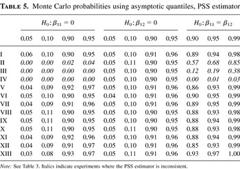
Monte Carlo probabilities using asymptotic quantiles, PSS
estimator
It can be seen from Table 3 that the
simulated probabilities are very close to the asymptotic probabilities
for the new estimator. Only in a few cases is the difference larger
than 3–4 percentage points. This suggests that asymptotic
critical values can be used when testing hypotheses about the index
coefficients, at least in samples of 200 observations or more.
Table 4 shows similar numbers for the Cox
estimator using the usual variance estimator based on the inverse
information matrix. As expected the simulated probabilities are
virtually identical to the asymptotic probabilities in experiments
I–IV where the Cox estimator is correctly specified and
consistent. Perhaps more surprisingly, the probabilities are not far
off for the t-tests in experiments V–VIII. However, the
simulated probabilities are very different from the asymptotic in all
other cases where the Cox estimator is inconsistent. Note that the
number of samples where the Cox estimator failed to converge is
extremely large in some experiments.
Table 5 contains results for the PSS
estimator using the variance estimator suggested by Powell et al.
(1989). The simulated probabilities here are
remarkably close to asymptotic probabilities in all experiments where
the PSS estimator is consistent and indeed are slightly better than
simulated probabilities for the new estimator. Note that the PSS
estimator is also consistent in the censored experiments II–IV
when β1 = (1,0)′, because the index coefficients
are the same for both risks. For the experiments where the PSS
estimator is inconsistent, the simulated probabilities are very
different from the asymptotic, as expected.
The conclusion of these Monte Carlo simulations is straightforward.
If the risk-specific hazard rates are known to be proportional, use
Cox's partial likelihood estimator. If such information is not
available, but the data are either single-risk or the censoring
mechanism is known to be independent of the explanatory variables and
the data are relatively free of outliers, there are two reasons to
favor the PSS estimator over the new estimator: the PSS estimator is
much faster to compute, and its variance estimator appears to have
slightly better properties. In other cases, such as nontrivial
competing risks data or data with outliers, the new estimator is
preferable.
6. CONCLUSION
This paper proposed a new semiparametric estimator of index
coefficients for a risk-specific hazard function. It is assumed that
the hazard function satisfies an index restriction, but no other
essential assumptions are imposed. In particular, the assumption of
proportional hazards is avoided. The new estimator is applicable to
competing risks data. Currently no other semiparametric estimator is
applicable to competing risks data without the assumption of
proportional hazards. The estimator described in this paper requires
that the explanatory variables be continuous; however, an estimator for
discrete explanatory variables is developed in a companion paper.
The index coefficient estimator was shown to be
root-n consistent and
asymptotically normally distributed, similarly to index coefficient
estimators developed for other settings. A consistent estimator of the
variance matrix was proposed. The paper also described how the index
restriction can be used to eliminate the curse of dimensionality in
nonparametric estimation.
The Monte Carlo simulations suggested that the new estimator performs
well in samples of 200 observations. The new estimator was compared
with Cox's partial likelihood estimator and the weighted average
derivative estimator of Powell et al. (1989).
Based on the Monte Carlo simulations it was possible to formulate
guidelines for when to use which estimator.
One large problem, the question of optimal bandwidth selection, was
left for future research. The approach taken by Härdle and
Tsybakov (1993) and Powell and Stoker (1996) for the weighted average derivative estimator
of Powell et al. (1989) seems promising, and
it may be to worthwhile to investigate whether it can be successfully
adapted to the present index coefficient estimator.
TECHNICAL APPENDIX
Proof of Theorem 1. Recall the definitions T =
(Y,S,X′)′ and t =
(y,s,x′)′. Let P denote
the distribution of T and let Pn
denote the empirical measure formed from the n independent
observations on P; that is, Pn
puts probability 1/n on each of the observations. Linear
functional notation is used throughout the Appendix. The expected value
of a random variable V is denoted EV,
.
Product measures are
denoted using the symbol [otimes ]. For example, P [otimes ]
Pf = Ef
(T1,T2) where
T1 and T2 are independent
random variables distributed as T.
Recall that
where ρ0 is defined in (15). Define also
To prove part i of the theorem, convergence is established for each
term in the decomposition
Note that
.
It follows immediately that
.
A change of variables implies that
ρ0(ti,tj)
=
Q01(ti,tj)
+
Q00(ti,tj),
where
Because
∂x1−dK and
w are bounded and
∂xdK is
integrable, Vn =
O(n−1b−q−1)
= o(n−1/2) almost surely
provided
n−1/2b−q−1
→ 0, or nb2q+2 → ∞, as
n → ∞.
By Lemma 3.1 of Powell et al. (1989),
provided
E(∥ρ1(Ti,Tj)∥2)
= op(n) for i ≠
j. (∥·∥ denotes the euclidean norm
∥u∥2 = [sum ]i
ui2 =
u′u.) To verify this condition, note that
Expanding
ρ0(ti,tj)′ρ0(ti,tj)
=
(Q01(ti,tj)
+
Q00(ti,tj))′(Q01(ti,tj)
+
Q00(ti,tj))
yields four terms that after a change of variables have the form
By further change of variables,
Similarly, the terms making up
ρ0(ti,tj)′ρ0(tj,ti)
have the form
Because
∂x1−djK,
ξ, and w are bounded and
∂xdjK
is integrable, these results imply
E(∥ρ1(Ti,Tj)∥2)
=
Op(b−q−2)
= op(n) provided that
nbq+2 → ∞ as n →
∞. Note that this is exactly the same as the condition derived by
Powell et al. (1989). It follows that the
limiting distribution of
is the same as the
limiting distribution of
.
By change of variables and integration by parts
where sup|r1| =
O(b) because ∂x w,
∂x2w,
∂x A2, and
∂x2A2 exist and
are bounded and K is integrable. Similarly,
where sup|r2| =
O(b) because
∂xjw and
∫|∂xjA1(dy,·,·)|
exist and are bounded for j = 1,2 and K is
integrable. It follows that
The second moment of
n1/2(Pn −
P)rj, j = 1,2, is
P(rj2) −
(Prj)2, which is bounded by
P(rj2) =
O(b2) using
sup|rj| =
O(b). It follows by Chebyshev's inequality that
(Pn −
P)rj =
op(n−1/2),
whence the limiting distribution of
is the same as the
limiting distribution of
.
Part i of the theorem now follows from the multivariate
Lindeberg–Lévy central limit theorem.
Turn now to the bias term. By previous arguments
By integration by parts and change of variables
Using the assumptions that
∫|∂xjA1(dy,·)|
and
∂xjA2
exist and are bounded and continuous for j =
1,…,k and that K is of order k, a
Taylor series expansion implies
Part ii of the theorem follows. █