


1 Introduction
Homological mirror symmetry was originally conceived by Kontsevich as an equivalence of the Fukaya category of a compact symplectic manifold with the bounded derived category of coherent sheaves on a mirror dual compact complex variety. Since then it has grown into a vast program connecting Fukaya categories of several kinds associated with not necessarily compact symplectic manifolds with derived categories of several kinds attached to possibly singular algebraic varieties.
In [Reference Lekili and PolishchukLP18], we proved a version of homological mirror symmetry relating Fukaya categories of punctured Riemann surfaces to some derived categories attached to stacky nodal curves. More precisely, for a punctured Riemann surface  $\unicode[STIX]{x1D6F4}$ and a line field
  $\unicode[STIX]{x1D702}$ on
  $\unicode[STIX]{x1D6F4}$, we choose a certain set of stops
  $\unicode[STIX]{x1D6EC}$, and consider the sequence of pre-triangulated categories
 $$\begin{eqnarray}\displaystyle {\mathcal{F}}(\unicode[STIX]{x1D6F4},\unicode[STIX]{x1D702})\rightarrow {\mathcal{W}}(\unicode[STIX]{x1D6F4},\unicode[STIX]{x1D6EC},\unicode[STIX]{x1D702})\rightarrow {\mathcal{W}}(\unicode[STIX]{x1D6F4},\unicode[STIX]{x1D702}), & & \displaystyle \nonumber\end{eqnarray}$$
 related by quasi-functors, where  ${\mathcal{F}}(\unicode[STIX]{x1D6F4},\unicode[STIX]{x1D702})$ is the compact Fukaya category [Reference SeidelSei08],
  ${\mathcal{W}}(\unicode[STIX]{x1D6F4},\unicode[STIX]{x1D6EC},\unicode[STIX]{x1D702})$ is the partially wrapped Fukaya category [Reference AurouxAur10a, Reference Haiden, Katzarkov and KontsevichHKK17], and
  ${\mathcal{W}}(\unicode[STIX]{x1D6F4},\unicode[STIX]{x1D702})$ is the (fully) wrapped Fukaya category [Reference Abouzaid and SeidelAS10]. The first functor is full and faithful, and the second functor is a localization functor corresponding to dividing by the full subcategory of Lagrangians supported near
  $\unicode[STIX]{x1D6EC}$.
On the mirror side, we consider a nodal stacky curve  $C$ obtained by attaching copies of weighted projective lines at their orbifold points (see [Reference Lekili and PolishchukLP18] for details), and we again have a sequence of categories
 $$\begin{eqnarray}\displaystyle \text{Perf}(C)\rightarrow D^{b}({\mathcal{A}}_{C})\rightarrow D^{b}\text{Coh}(C), & & \displaystyle \nonumber\end{eqnarray}$$
 where  ${\mathcal{A}}_{C}$ is a sheaf of algebras, called the Auslander order over
  $C$, that was previously studied in [Reference Burban and DrozdBD11]. We again have that the first functor is full and faithful, and the second functor is a localization. The main result of [Reference Lekili and PolishchukLP18] is an equivalence of homologically smooth and proper pre-triangulated categories
 $$\begin{eqnarray}\displaystyle {\mathcal{W}}(\unicode[STIX]{x1D6F4},\unicode[STIX]{x1D6EC},\unicode[STIX]{x1D702})\simeq D^{b}({\mathcal{A}}_{C}). & & \displaystyle\end{eqnarray}$$
It is proved by constructing a generating set of objects on each side and matching their endomorphism algebras. The main point is that these algebras turn out to be formal (in fact, concentrated in degree 0), which means that we only need to prove an isomorphism of the usual associative algebras and do not have to worry about higher products.
One then deduces an equivalence  ${\mathcal{W}}(\unicode[STIX]{x1D6F4},\unicode[STIX]{x1D702})\simeq D^{b}\text{Coh}(C)$ by identifying the subcategories on both sides of the equivalence (1.1) with respect to which to take the quotient. The equivalence
  ${\mathcal{F}}(\unicode[STIX]{x1D6F4},\unicode[STIX]{x1D702})\simeq \text{Perf}(C)$ is deduced by characterizing both sides as subcategories of the two sides of (1.1). Note that considering the same generators in the localized categories leads to differential graded (dg) algebras which are far from formal. Note also that the embedding
  $\text{Perf}(C){\hookrightarrow}D^{b}({\mathcal{A}}_{C})$ is a simple example of categorical resolutions considered in [Reference Kuznetsov and LuntsKL15].
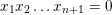
Let us explain this in more detail in a simple case. Let  $\unicode[STIX]{x1D6F4}$ be the pair of pants, that is, a three-punctured sphere, and let
  $\unicode[STIX]{x1D6EC}$ be two stops at the outer boundary as drawn in Figure 1. We also choose a line field
  $\unicode[STIX]{x1D702}$ on
  $\unicode[STIX]{x1D6F4}$ which has rotation number 2 around the outer boundary and 0 along the interior boundary components (see [Reference Lekili and PolishchukLP20] for a recent detailed study of line fields on punctured surfaces).
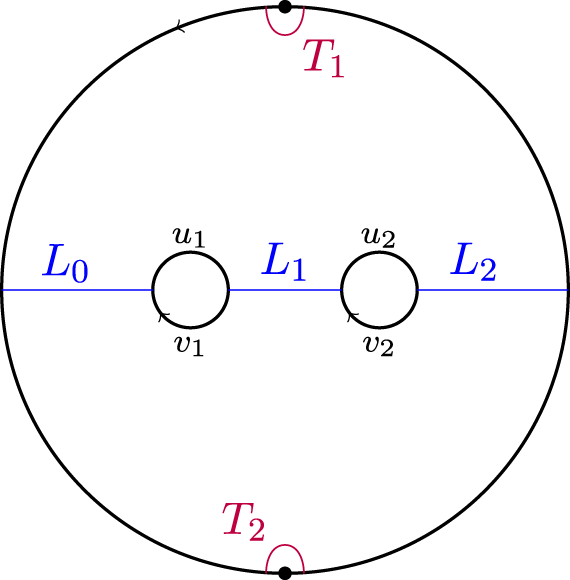
Figure 1. Pair of pants.
The partially wrapped Fukaya category  ${\mathcal{W}}(\unicode[STIX]{x1D6F4},\unicode[STIX]{x1D6EC},\unicode[STIX]{x1D702})$ is generated by the Lagrangians
  $L_{0},L_{1},L_{2}$ shown in Figure 1, and their endomorphism algebra is easily computed to be given by the quiver with relations on Figure 2.
Figure 2. Endomorphism algebra of a generating set.
On the B-side, the mirror is given by the Auslander order  $A$ over the node algebra
 $$\begin{eqnarray}\displaystyle R=\mathbf{k}[x_{1},x_{2}]/(x_{1}x_{2}), & & \displaystyle \nonumber\end{eqnarray}$$
 where  $\mathbf{k}$ is a commutative ring. The Auslander order in this case is simply
 $$\begin{eqnarray}\displaystyle A=\text{End}_{R}(R/(x_{1})\oplus R/(x_{2})\oplus R). & & \displaystyle \nonumber\end{eqnarray}$$
 One can directly see that  $A$ is isomorphic to the quiver algebra given in Figure 2. Note that
  $R$ is a Cohen–Macaulay algebra and the modules
  $R$,
$R$,  $R/(x_{1})$,
  $R/(x_{2})$ comprise the set of indecomposable maximal Cohen–Macaulay modules of
  $R$, and they generate
  $D^{b}(A)$ as a triangulated category, provided
  $\mathbf{k}$ is regular.
Now, the wrapped Fukaya category  ${\mathcal{W}}(\unicode[STIX]{x1D6F4},\unicode[STIX]{x1D702})$ is the localization of
  ${\mathcal{W}}(\unicode[STIX]{x1D6F4},\unicode[STIX]{x1D6EC},\unicode[STIX]{x1D702})$ given by dividing out by the subcategory generated by the objects
  $T_{1},T_{2}$ supported near the stops. We can express them in terms of
  $L_{0},L_{1},L_{2}$ as follows:
 $$\begin{eqnarray}\displaystyle T_{1} & \simeq & \displaystyle \{L_{0}\xrightarrow[{}]{u_{1}}L_{1}\xrightarrow[{}]{u_{2}}L_{2}\},\nonumber\\ \displaystyle T_{2} & \simeq & \displaystyle \{L_{2}\xrightarrow[{}]{v_{2}}L_{1}\xrightarrow[{}]{v_{1}}L_{0}\}.\nonumber\end{eqnarray}$$
 Similarly,  $D^{b}(R)$ is the localization of
  $D^{b}(A)$ obtained by dividing out by the corresponding subcategory, and this allows one to establish an equivalence
 $$\begin{eqnarray}\displaystyle {\mathcal{W}}(\unicode[STIX]{x1D6F4},\unicode[STIX]{x1D702})\simeq D^{b}(R). & & \displaystyle \nonumber\end{eqnarray}$$
1.1 New results
In this paper we apply the above strategy to prove homological mirror symmetry for the higher-dimensional pair of pants,
 $$\begin{eqnarray}\displaystyle {\mathcal{P}}_{n}=\text{Sym}^{n}(\mathbb{P}^{1}\setminus \{p_{0},p_{1},\ldots ,p_{n+1}\}), & & \displaystyle \nonumber\end{eqnarray}$$
 where  $\text{Sym}^{n}(\unicode[STIX]{x1D6F4})=\unicode[STIX]{x1D6F4}^{n}/\mathfrak{S}_{n}$ (see § 2 for a brief review of the symplectic topology of these spaces). In other words, the
  $n$-dimensional pair of pants is the complement of
  $(n+2)$ generic hyperplanes in
  $\mathbb{P}^{n}$.
On the A-side, we first introduce a stop  $\unicode[STIX]{x1D6EC}=\unicode[STIX]{x1D6EC}_{1}\cup \unicode[STIX]{x1D6EC}_{2}$, where
  $\unicode[STIX]{x1D6EC}_{i}=\{q_{i}\}\times \text{Sym}^{n-1}(\unicode[STIX]{x1D6F4})$ for some base points
  $q_{1},q_{2}$. We pick a grading structure
  $\unicode[STIX]{x1D702}$ and consider the partially wrapped Fukaya category
  ${\mathcal{W}}({\mathcal{P}}_{n},\unicode[STIX]{x1D6EC},\unicode[STIX]{x1D702})$, where we use some commutative ring
  $\mathbf{k}$ as coefficients. There is a natural generating set of objects
  $\{L_{S}:S\subset \{0,1,\ldots ,n+1\},|S|=n\}$ in this category and our first result is an explicit computation of the algebra of morphisms between these objects. In fact, we do this more generally for the symplectic manifolds
 $$\begin{eqnarray}\displaystyle M_{n,k}=\text{Sym}^{n}(\mathbb{P}^{1}\setminus \{p_{0},p_{1},\ldots ,p_{k}\}); & & \displaystyle \nonumber\end{eqnarray}$$
see Theorem 3.2.5 for the precise description of the resulting algebra.
Next, we specialize to the case  $k=n+1$. In this case, on the B-side we consider the categorical resolutions of the algebra
 $$\begin{eqnarray}\displaystyle R=\mathbf{k}[x_{1},x_{2},\ldots ,x_{n+1}]/(x_{1}x_{2}\ldots x_{n+1}) & & \displaystyle \nonumber\end{eqnarray}$$
given by
 $$\begin{eqnarray}\displaystyle {\mathcal{B}}^{\circ }:=\operatorname{End}_{R}(R/(x_{1})\oplus R/(x_{[1,2]})\oplus \cdots \oplus R/(x_{[1,n]})\oplus R) & & \displaystyle \nonumber\end{eqnarray}$$
and
 $$\begin{eqnarray}\displaystyle {\mathcal{B}}^{\circ \circ }:=\operatorname{End}_{R}\biggl(\bigoplus _{I\subset [1,n+1],I\neq \emptyset }R/(x_{I})\biggr), & & \displaystyle \nonumber\end{eqnarray}$$
 where the summation is over all non-empty subintervals of  $[1,n+1]$, and for
  $I\subset [1,n+1]$ we use the notation
  $x_{I}:=\prod _{i\in I}x_{i}$.
By explicit computations we prove the following theorem (see Theorem 5.2.1).
Theorem 1.1.1. There exists a grading structure  $\unicode[STIX]{x1D702}$ on
  ${\mathcal{P}}_{n}$ such that we have an equivalence of pre-triangulated categories over
  $\mathbf{k}$,
 $$\begin{eqnarray}\displaystyle {\mathcal{W}}({\mathcal{P}}_{n},\unicode[STIX]{x1D6EC},\unicode[STIX]{x1D702})\simeq \operatorname{Perf}({\mathcal{B}}^{\circ \circ }). & & \displaystyle \nonumber\end{eqnarray}$$
We next analyze the localization of these categories corresponding to dividing out by objects supported near the stops to deduce homological mirror symmetry for the (fully) wrapped Fukaya categories.
Corollary 1.1.2. For the same grading structure  $\unicode[STIX]{x1D702}$ we have equivalences of pre-triangulated categories over
  $\mathbf{k}$:
 $$\begin{eqnarray}\displaystyle {\mathcal{W}}({\mathcal{P}}_{n},\unicode[STIX]{x1D6EC}_{1},\unicode[STIX]{x1D702})\simeq \operatorname{Perf}({\mathcal{B}}^{\circ }). & & \displaystyle \nonumber\end{eqnarray}$$
 Assume that  $\mathbf{k}$ is a regular ring. Then we also have an equivalence
 $$\begin{eqnarray}\displaystyle {\mathcal{W}}({\mathcal{P}}_{n},\unicode[STIX]{x1D702})\simeq D^{b}\text{Coh}(x_{1}x_{2}\ldots x_{n+1}=0). & & \displaystyle \nonumber\end{eqnarray}$$
 Finally, we deduce similar equivalences for finite abelian covers of  ${\mathcal{P}}_{n}$, associated with homomorphisms
  $\unicode[STIX]{x1D70B}_{1}({\mathcal{P}}_{n})\simeq \mathbb{Z}^{n+1}\rightarrow \unicode[STIX]{x1D6E4}$ into finite abelian groups
  $\unicode[STIX]{x1D6E4}$. On the B-side we take equivariant versions of the above categories with respect to the natural actions of the dual finite commutative group scheme
  $G=\unicode[STIX]{x1D6E4}^{\ast }$ (see Theorem 5.3.3).
Note that to prove the homological mirror symmetry statement (the second equivalence of Corollary 1.1.2), it is enough to work with one stop  $\unicode[STIX]{x1D6EC}_{1}$. The reason we consider the picture with two stops is due to the relation with the Auslander order discussed above and to Ozsváth and Szabó’s bordered algebras (see also Remarks 5.3.5 and 3.2.7).
1.2 Relation to other works
Homological mirror symmetry for pair of pants is a much studied subject. However, a complete proof of Corollary 1.1.2 has not appeared in writing until this paper. A motivation for studying these particular examples of mirror symmetry comes from a theorem of Mikhalkin [Reference MikhalkinMik04] that a hypersurface in  $\mathbb{C}P^{n+1}$ admits a decomposition into several
  ${\mathcal{P}}_{n}$, much like a Riemann surface admits a decomposition into several
  ${\mathcal{P}}_{1}$.
In [Reference SheridanShe11], Sheridan identifies the mirror (immersed) Lagrangian in  ${\mathcal{P}}_{n}$ corresponding to
  ${\mathcal{O}}_{0}$, the structure sheaf of the origin in the triangulated category of singularities of the normal crossing divisor
  $x_{0}x_{1}x_{2}\ldots x_{n+1}=0$ in
  $\mathbb{C}^{n+2}$. By a theorem of Orlov [Reference OrlovOrl04], the latter category is quasi-equivalent to the matrix factorization category
  $\text{mf}(\mathbb{C}^{n+2},x_{0}x_{1}x_{2}\ldots x_{n+1})$. Note that by the result of Isik [Reference IsikIsi13], the latter category (or more precisely, its
  $\mathbb{G}_{m}$-equivariant version where
  $x_{1},\ldots ,x_{n+1}$ have weight 0 and
  $x_{0}$ has weight 2) is naturally quasi-equivalent to the derived category of
  $x_{1}x_{2}\ldots x_{n+1}=0$ (see also [Reference ShipmanShi12]). Under this equivalence,
  ${\mathcal{O}}_{0}$ corresponds to a perfect object supported at the origin.
In [Reference NadlerNad16], instead of the wrapped Fukaya category of  ${\mathcal{P}}_{n}$, Nadler studies the
  $\mathbb{Z}_{2}$-graded category of wrapped microlocal sheaves associated to a skeleton of
  ${\mathcal{P}}_{n}$ (see also the follow-up paper by Gammage and Nadler [Reference Gammage and NadlerGN20]). It is then verified that this category agrees with the
  $\mathbb{Z}_{2}$-graded category of matrix factorizations
  $\text{mf}(\mathbb{C}^{n+2},x_{0}x_{1}x_{2}\ldots x_{n+1})$. It is expected and in certain cases proved that the wrapped microlocal sheaves category is equivalent to the wrapped Fukaya category (see [Reference Ganatra, Pardon and ShendeGPS18b] for the case of cotangent bundles). However, such an equivalence for arbitrary Weinstein manifolds has not yet been accomplished. Nonetheless, in view of the works of Ganatra, Pardon and Shende [Reference Ganatra, Pardon and ShendeGPS19, Reference Ganatra, Pardon and ShendeGPS18a, Reference Ganatra, Pardon and ShendeGPS18b], such an equivalence in the case of
  ${\mathcal{P}}_{n}$ seems to be within reach (see, in particular, the discussion in [Reference Ganatra, Pardon and ShendeGPS18b, § 6.6] which outlines a proof depending on work in progress). Establishing such an equivalence for
  ${\mathcal{P}}_{n}$ would give another confirmation for Corollary 1.1.2 (at least in the
  $\mathbb{Z}_{2}$-graded case).
The work closest to ours is [Reference AurouxAur18], in which Auroux sketches a proof of homological mirror symmetry for  ${\mathcal{P}}_{n}$ which depends on certain conjectures about generation by an explicit collection of Lagrangians and a classification of
  $A_{\infty }$-structures on their cohomology.
We also mention that partially wrapped Fukaya categories of symmetric products appear predominantly in Heegaard Floer homology [Reference Lipshitz, Ozsváth and ThurstonLOT18, Reference AurouxAur10a, Reference AurouxAur10b] (see also [Reference Lekili and PerutzLP11]). In particular, our computations of  ${\mathcal{W}}(M_{n,k})$ give an alternative viewpoint for knot Floer homology. We defer this to a future work.
This paper is organized as follows. After reviewing some background material on partially wrapped Fukaya categories of symmetric powers of Riemann surfaces in § 2, we present the computation of the algebra of morphisms between generating Lagrangians in  $M_{n,k}$ in § 3. Then in § 4 we deal with the B-side of the story: we study the derived categories of modules over
  ${\mathcal{B}}^{\circ }$ and
  ${\mathcal{B}}^{\circ \circ }$. In particular, we construct semiorthogonal decompositions of these categories and obtain localization results similar to those corresponding to the removal of a stop on the A-side. Finally, in § 5 we prove the equivalences of categories on the A-side and on the B-side (see Theorem 5.2.1).
Conventions. We work over a base commutative ring  $\mathbf{k}$. When we write complexes of modules in the form
  $[\ldots \rightarrow \cdot ]$, we assume that the rightmost term sits in degree
  $0$. The morphism complexes in dg-categories are denoted by lowercase
  $\text{hom}$, while their cohomology are denoted by
  $\operatorname{Hom}^{\bullet }$. We also abbreviate
  $\operatorname{Hom}^{0}$ simply as
  $\operatorname{Hom}$. The wrapped Fukaya category we consider is defined as the split-closed pre-triangulated envelope of the category whose objects are graded exact Lagrangians.
2 A brief review of Fukaya categories of symmetric products of Riemann surfaces
Let  $\unicode[STIX]{x1D6F4}$ be a Riemann surface. For each
  $n>0$, there exists a smooth
  $n$-dimensional complex algebraic variety
 $$\begin{eqnarray}\displaystyle \operatorname{Sym}^{n}(\unicode[STIX]{x1D6F4}):=\unicode[STIX]{x1D6F4}^{n}/\mathfrak{S}_{n}, & & \displaystyle\end{eqnarray}$$
 where  $\mathfrak{S}_{n}$ is the permutation group which acts by permuting the components of the product.
Let  $\unicode[STIX]{x1D70B}:\unicode[STIX]{x1D6F4}^{n}\rightarrow \operatorname{Sym}^{n}(\unicode[STIX]{x1D6F4})$ be the branched covering map. Fix an area form
  $\unicode[STIX]{x1D714}$ on
  $\unicode[STIX]{x1D6F4}$. In [Reference PerutzPer08, § 7], Perutz explains how to smoothen the closed current
  $\unicode[STIX]{x1D70B}_{\ast }(\unicode[STIX]{x1D714}^{\times n})$ on
  $\operatorname{Sym}^{n}(\unicode[STIX]{x1D6F4})$ to a Kähler form
  $\unicode[STIX]{x1D6FA}$ by modifying it in an arbitrarily small analytic neighborhood of the (big) diagonal. In particular, outside this neighborhood we have
  $\unicode[STIX]{x1D6FA}=\unicode[STIX]{x1D70B}_{\ast }(\unicode[STIX]{x1D714}^{\times n})$. Throughout, we will view
  $\operatorname{Sym}^{n}(\unicode[STIX]{x1D6F4})$ as a symplectic manifold equipped with such a Kähler form
  $\unicode[STIX]{x1D6FA}$.
If we write  $g=g(\unicode[STIX]{x1D6F4})$ for the genus of
  $\unicode[STIX]{x1D6F4}$, the first Chern class of such a variety is given by
 $$\begin{eqnarray}\displaystyle c_{1}(\operatorname{Sym}^{n}(\unicode[STIX]{x1D6F4}))=(n+1-g)\unicode[STIX]{x1D702}-\unicode[STIX]{x1D703}, & & \displaystyle \nonumber\end{eqnarray}$$
 where  $\unicode[STIX]{x1D702}$ and
  $\unicode[STIX]{x1D703}$ are the Poincaré duals of the class
  $\{pt\}\times \operatorname{Sym}^{n-1}(\unicode[STIX]{x1D6F4})$ and the theta divisor, respectively. These two cohomology classes span the invariant part of
  $H^{2}(\operatorname{Sym}^{n}(\unicode[STIX]{x1D6F4}))$ under the action of the mapping class group of
  $\unicode[STIX]{x1D6F4}$. Moreover, we have that
  $[\unicode[STIX]{x1D6FA}]=\unicode[STIX]{x1D702}$.
In particular, when
 $$\begin{eqnarray}\displaystyle \unicode[STIX]{x1D6F4}=\mathbb{P}^{1}\setminus \{p_{0},p_{1},\ldots ,p_{k}\}, & & \displaystyle\end{eqnarray}$$
 $\operatorname{Sym}^{n}(\unicode[STIX]{x1D6F4})$ is an exact symplectic manifold with
  $c_{1}=0$. Such symplectic manifolds are sometimes referred to as symplectically Calabi–Yau manifolds, and their Fukaya categories can be
  $\mathbb{Z}$-graded [Reference SeidelSei00]. From the point of view of symplectic topology, the positions of the points do not matter, so let us introduce the notation
 $$\begin{eqnarray}\displaystyle M_{n,k}=\operatorname{Sym}^{n}(\mathbb{P}^{1}\setminus \{p_{0},p_{1},\ldots ,p_{k}\}) & & \displaystyle\end{eqnarray}$$
 to denote the exact symplectic manifold with  $c_{1}=0$. The grading structures are given by homotopy classes of trivializations of the bicanonical bundle, and there is an effective
  $H^{1}(\operatorname{Sym}^{n}(\unicode[STIX]{x1D6F4}))\simeq H^{1}(\unicode[STIX]{x1D6F4})$ worth of choices.
Recall the well-known isomorphism of algebraic varieties
 $$\begin{eqnarray}\displaystyle \operatorname{Sym}^{n}(\mathbb{P}^{1})\simeq \mathbb{P}^{n} & & \displaystyle\end{eqnarray}$$
 given by sending an effective divisor of degree  $n$ on
  $\mathbb{P}^{1}$ to its homogeneous equation defined up to rescaling.
Therefore, one can think of  $M_{n,k}$ as the complement of
  $k+1$ generic hyperplanes in
  $\mathbb{P}^{n}$. This provides an alternative way to equip
  $M_{n,k}$ with a symplectic structure by viewing it as an affine variety, but we will not pursue this any further, as we prefer to emphasize the structure of
  $M_{n,k}$ as a symmetric product on a punctured surface of genus 0. The two symplectic structures are equivalent as they both tame the standard complex structure
  $J=\text{Sym}^{n}(j)$ on
  $M_{n,k}$ induced from
  $\mathbb{P}^{n}$ (see [Reference PerutzPer08, Proposition 1.1]). This also makes it clear that for
  $0\leqslant k<n$,
  $M_{n,k}=\mathbb{C}^{n-k}\times \mathbb{\{}^{k}$, which is a subcritical Stein manifold, so our main interest will be in
  $k\geqslant n$.
We will also equip  $M_{n,k}$ with stops
  $\unicode[STIX]{x1D6EC}_{Z}$ corresponding to a choice of symplectic hypersurfaces of the form
  $\{p\}\times \operatorname{Sym}^{n-1}(\unicode[STIX]{x1D6F4})$ for
  $p\in Z$, where
  $Z$ is finite set of points. The set
  $Z$ will be indicated by choosing stops in the ideal boundary of
  $\unicode[STIX]{x1D6F4}$. More precisely, by removing cylindrical ends, we view
  $\unicode[STIX]{x1D6F4}$ as a two-dimensional surface with boundary and the set
  $Z$ will be chosen as a finite set of points on
  $\unicode[STIX]{x2202}\unicode[STIX]{x1D6F4}$.
We write  ${\mathcal{W}}(M_{n,k},\unicode[STIX]{x1D6EC}_{Z})$ for the partially wrapped Fukaya category. Motivated by bordered Heegaard Floer homology [Reference Lipshitz, Ozsváth and ThurstonLOT18], these categories were originally constructed by Auroux in [Reference AurouxAur10a, Reference AurouxAur10b]. These works provide foundational results on these categories, as well as some very useful results about generating objects and the existence of certain exact triangles.
All of the Lagrangians that we use will be of the form  $L_{1}\times L_{2}\times \cdots \times L_{n}$, where
  $L_{i}\subset \unicode[STIX]{x1D6F4}$ are pairwise disjoint Lagrangian arcs in
  $\unicode[STIX]{x1D6F4}$, which can be considered as objects in
  ${\mathcal{W}}(\unicode[STIX]{x1D6F4},Z)$. Auroux proves in [Reference AurouxAur10b, Theorem 1] that, given a set of Lagrangians
  $L_{0},L_{1},\ldots ,L_{k}$ such that their complement in
  $\unicode[STIX]{x1D6F4}$ is a disjoint union of disks with at most one stop in their boundary, for
  $1\leqslant n\leqslant k+1$, the corresponding partially wrapped Fukaya category of
  $\operatorname{Sym}^{n}(\unicode[STIX]{x1D6F4})$ is generated by
  $\binom{k+1}{n}$ product Lagrangians
  $L_{i_{1}}\times \cdots \times L_{i_{n}}$, where
  $(i_{1},\ldots ,i_{n})$ runs through subsets of
  $\{0,1,\ldots ,k\}$ of size
  $n$. Notice that this generation result only depends on the configuration of
  $L_{i}$ on
  $\unicode[STIX]{x1D6F4}$ and is independent of
  $n$.
$n$.
Furthermore, Auroux explains how to compute the dg-endomorphism algebra for such product Lagrangians (see [Reference AurouxAur10b, Proposition 11]; note that there are no higher products). As vector spaces, the morphism spaces are defined by
 $$\begin{eqnarray}\displaystyle & & \displaystyle \text{hom}(L_{i_{1}}\times L_{i_{2}}\times \cdots \times L_{i_{n}},L_{j_{1}}\times L_{j_{2}}\times \cdots \times L_{j_{n}})\nonumber\\ \displaystyle & & \displaystyle \quad =\bigoplus _{\unicode[STIX]{x1D70E}}\text{hom}(L_{i_{1}},L_{\unicode[STIX]{x1D70E}(i_{1})})\,\otimes \,\text{hom}(L_{i_{2}},L_{\unicode[STIX]{x1D70E}(i_{2})})\,\otimes \,\cdots \,\otimes \,\text{hom}(L_{i_{n}},L_{\unicode[STIX]{x1D70E}(i_{n})}),\nonumber\end{eqnarray}$$
 where  $\unicode[STIX]{x1D70E}$ runs through bijections
  $\{i_{1},\ldots ,i_{n}\}\rightarrow \{j_{1},\ldots ,j_{n}\}$.
Following [Reference Lipshitz, Ozsváth and ThurstonLOT18], we can represent these generators via strand diagrams as follows. First, the endpoints of the Lagrangians  $L_{i_{1}},\ldots ,L_{i_{n}}$,
  $L_{j_{1}},\ldots ,L_{j_{n}}$ are grouped into equivalence classes according to which boundary component of
  $\unicode[STIX]{x1D6F4}$ they end on. Note that the set of endpoints lying on each boundary component has a cyclic order induced by the orientation of the boundary. Thus, given a morphism
  $(f_{1},\ldots f_{n})$, we can assume that it is of the form
  $(f_{i_{1},1},\ldots ,f_{i_{r_{1}},1},f_{i_{1},2},\ldots ,f_{i_{r_{2}},2}\ldots ,f_{i_{1},k},\ldots ,f_{i_{r_{k}},k})$ where
  $f_{i_{1},s},\ldots ,f_{i_{r_{s}},s}$ are Reeb chords along the
  $s$th boundary component
  $\unicode[STIX]{x2202}\unicode[STIX]{x1D6F4}_{s}\subset \unicode[STIX]{x2202}\unicode[STIX]{x1D6F4}$, where the Reeb flow is simply the rotation along the orientation of the boundary. Thus, each
  $f_{i_{j},s}$ either represents the idempotent of the corresponding Lagrangian
  $L_{i_{j},s}$ or goes in the strictly positive direction along
  $\unicode[STIX]{x2202}\unicode[STIX]{x1D6F4}_{s}$. Thus, the set of Reeb chords
  $f_{i_{1},s},\ldots ,f_{i_{r_{s}},s}$ can be represented in
  $\mathbb{R}\times [0,1]$ as upward veering strands from
  $\mathbb{R}\times \{0\}$ to
  $\mathbb{R}\times \{1\}$, or as a straight horizontal line if it corresponds to an idempotent. Here,
  $\mathbb{R}$ is the universal cover of the component
  $\unicode[STIX]{x2202}\unicode[STIX]{x1D6F4}_{s}$ and
  $[0,1]$ is the time direction (see Figure 3).

Figure 3. A strand diagram with three boundary components.
In the case where a boundary component contains stops the Reeb chords are not allowed to pass through the stops. Hence, instead of using the universal cover  $\mathbb{R}$, one cuts along the stops and uses the subintervals to draw the strand diagram. We do not elaborate on the notation to describe this.
Now, the product in  ${\mathcal{W}}(M_{n,k},\unicode[STIX]{x1D6EC}_{Z})$ is induced by the composition in
  ${\mathcal{W}}(\unicode[STIX]{x1D6F4},Z)$. Namely, we have
 $$\begin{eqnarray}\displaystyle (f_{1}\,\otimes \,\cdots \,\otimes \,f_{n})\circ (g_{1}\,\otimes \,\cdots \,\otimes \,g_{n})=(f_{1}g_{\unicode[STIX]{x1D70E}(1)}\,\otimes \,f_{2}g_{\unicode[STIX]{x1D70E}(2)}\,\otimes \,\cdots \,\otimes \,f_{n}g_{\unicode[STIX]{x1D70E}(n)}) & & \displaystyle \nonumber\end{eqnarray}$$
 if there exists a  $\unicode[STIX]{x1D70E}\in \mathfrak{S}_{n}$ such that all the compositions
  $f_{i}g_{\unicode[STIX]{x1D70E}(i)}$ in
  ${\mathcal{W}}(\unicode[STIX]{x1D6F4},Z)$ are non-zero, and with the additional important condition that in the strand representation no two strands of the concatenated diagram cross more than once; otherwise the product is set to be zero (see Figure 4).

Figure 4. A strand diagram with two strands crossing more than once.
The differential on the space of morphisms is defined as the sum of all the ways of resolving one crossing of the strand diagram excluding resolutions in which two strands intersect twice (see Figure 5).

Figure 5. Resolution of strand diagram.
In this way we get an explicit dg-category, quasi-equivalent to  ${\mathcal{W}}(M_{n,k},\unicode[STIX]{x1D6EC}_{Z})$. In what follows, we use these results without further explanations.
We can choose a line field to give  ${\mathcal{W}}(\unicode[STIX]{x1D6F4},Z)$ a
  $\mathbb{Z}$-grading (see [Reference Lekili and PolishchukLP20] for a recent study of this structure). There are effectively
  $H^{1}(\unicode[STIX]{x1D6F4})$ worth of choices for the line field. The set of grading structures for
  $M_{n,k}$ is a torsor for an isomorphic group
  $H^{1}(\operatorname{Sym}^{n}(\unicode[STIX]{x1D6F4}))\cong H^{1}(\unicode[STIX]{x1D6F4})$. However, the relation between grading structures on
  $\unicode[STIX]{x1D6F4}$ and on
  $\operatorname{Sym}^{n}(\unicode[STIX]{x1D6F4})$ seems to be quite subtle: it is easy to see that the grading of a morphism
  $(f_{1}\,\otimes \,\cdots \,\otimes \,f_{n})$ in
  ${\mathcal{W}}(M_{n,k},\unicode[STIX]{x1D6EC}_{Z})$ cannot be given by the sum of the gradings of morphisms
  $f_{i}$ in
  ${\mathcal{W}}(\unicode[STIX]{x1D6F4},Z)$. For example, we will encounter objects
  $L_{1},L_{2}$ and morphisms
  $u\in \operatorname{hom}(L_{1},L_{2})$ and
  $v\in \operatorname{hom}(L_{2},L_{1})$ such that
 $$\begin{eqnarray}\displaystyle \unicode[STIX]{x2202}(\operatorname{id}_{L_{1}}\,\otimes \,uv)=\unicode[STIX]{x2202}(vu\,\otimes \,\operatorname{id}_{L_{2}})=v\,\otimes \,u\in \operatorname{hom}(L_{1}\times L_{2},L_{1}\times L_{2}). & & \displaystyle \nonumber\end{eqnarray}$$
 This makes direct determination of the gradings in  ${\mathcal{W}}(M_{n,k},\unicode[STIX]{x1D6EC}_{Z})$ difficult. Instead, we are able to pin down the grading structures on
  $M_{n,k}$ using an explicit calculation of the endomorphism algebra of a generating set of Lagrangians.
Finally, we recall a basic exact triangle from [Reference AurouxAur10a, Lemma 5.2]. Let us consider the Lagrangians  $L=L_{1}\times L_{2}\times \cdots \times L_{n}$,
  $L^{\prime }=L_{1}^{\prime }\times L_{2}\times \cdots \times L_{n}$, and
  $L^{\prime \prime }=L_{1}^{\prime \prime }\times L_{2}\times \cdots \times L_{n}$, where
  $L_{1}^{\prime \prime }$ is the arc obtained by sliding
  $L_{1}$ along
  $L_{1}^{\prime }$. Then
  $L$,
$L$,  $L^{\prime }$ and
  $L^{\prime \prime }$ fit into an exact triangle
 $$\begin{eqnarray}\displaystyle L\overset{u\,\otimes \,\operatorname{id}}{\longrightarrow }L^{\prime }\rightarrow L^{\prime \prime }\rightarrow L[1] & & \displaystyle\end{eqnarray}$$
coming from an exact triangle
 $$\begin{eqnarray}\displaystyle L_{1}\overset{u}{\longrightarrow }L_{1}^{\prime }\rightarrow L_{1}^{\prime \prime }\rightarrow L_{1}[1] & & \displaystyle \nonumber\end{eqnarray}$$
 in  ${\mathcal{W}}(\unicode[STIX]{x1D6F4},Z)$.
Similarly, if  $L=L_{1}\times L_{2}\times \cdots \times L_{n}$ and
  $L^{\prime }=L_{1}^{\prime }\times L_{2}\times \cdots \times L_{n}$, where
  $L_{1}^{\prime }$ is obtained by sliding
  $L_{1}$ along
  $L_{2}$, then
  $L$ and
  $L^{\prime }$ are isomorphic in the category
  ${\mathcal{W}}(M_{n,k},\unicode[STIX]{x1D6EC}_{Z})$. Indeed, in this situation one can show that
  $L$ and
  $L^{\prime }$ are Hamiltonian isotopic (see [Reference PerutzPer08, Reference AurouxAur10a]).
3 A-side
Throughout, we will work over a commutative ring  $\mathbf{k}$. We consider the sphere
  $\unicode[STIX]{x1D6F4}_{k}$ with
  $k+1$ holes and two stops
  $Z=q_{1}\cup q_{2}$ on one of the boundary components. We have a generating set of Lagrangians
  $L_{0}$,
  $L_{1},\ldots ,L_{k}$, which connect the
  $i$th hole to the
  $(i+1)$th hole for
  $i\in \mathbb{Z}/(k+1)$ (see Figure 6 for
  $k=3$). As in Figure 6, we view
  $\unicode[STIX]{x1D6F4}_{k}$ as a
  $k$-holed disk. We call the punctures that lie in the interior of the disk the interior punctures of
  $\unicode[STIX]{x1D6F4}_{k}$ and label them
  $1,2,\ldots ,k$ from left to right. We call the unique puncture that corresponds to the boundary of the disk the exterior puncture of
  $\unicode[STIX]{x1D6F4}_{k}$ and label it
  $0$.
$0$.
Let  $M_{n,k}=\operatorname{Sym}^{n}(\unicode[STIX]{x1D6F4}_{k})$ and
  $\unicode[STIX]{x1D6EC}=\unicode[STIX]{x1D6EC}_{Z}=\unicode[STIX]{x1D6EC}_{1}\cup \unicode[STIX]{x1D6EC}_{2}$ be the corresponding stops. Thus,
  $\unicode[STIX]{x1D6EC}_{i}=q_{i}\times \operatorname{Sym}^{n-1}(\unicode[STIX]{x1D6F4}_{k})$ are symplectic hypersurfaces in
  $M_{n,k}$.
The objects  $L_{0},\ldots ,L_{k}$ generate the partially wrapped Fukaya category
  ${\mathcal{W}}(\unicode[STIX]{x1D6F4},Z)$. Furthermore, by Auroux’s theorem [Reference AurouxAur10b, Theorem 1], the category
  ${\mathcal{W}}(M_{n,k},\unicode[STIX]{x1D6EC})$ is generated by the Lagrangians
 $$\begin{eqnarray}\displaystyle L_{S}=L_{i_{1}}\times L_{i_{2}}\times \cdots \times L_{i_{n}}, & & \displaystyle \nonumber\end{eqnarray}$$
 where  $i_{j}\in S$ and
  $S$ is a subset of
  $[0,k]$ of size
  $n$.
$n$.
Below we will describe the algebra
 $$\begin{eqnarray}\displaystyle {\mathcal{A}}^{\circ \circ }=\bigoplus _{S,S^{\prime }}\operatorname{Hom}_{{\mathcal{W}}(M_{n,k},\unicode[STIX]{x1D6EC})}(L_{S},L_{S^{\prime }}). & & \displaystyle\end{eqnarray}$$
 It will turn out that for  $n<k$,
  ${\mathcal{A}}^{\circ \circ }$ is in fact an
  $R$-algebra, where
 $$\begin{eqnarray}\displaystyle R=\mathbf{k}[x_{1},\ldots ,x_{k}]/(x_{1}\ldots x_{k}). & & \displaystyle\end{eqnarray}$$
 Here  $x_{i}$ will correspond to the closed Reeb orbit around the
  $i$th interior puncture of
  $\unicode[STIX]{x1D6F4}_{k}$.

Figure 6. Sphere with four holes, two stops, a generating set of Lagrangians ( $L_{i}$) and certain other Lagrangians supported near stops (
 $T_{1}$ and
  $T_{2}$).
At the  $i$th interior puncture, we write
  $u_{i},v_{i}$ for the two primitive Reeb chords
 $$\begin{eqnarray}\displaystyle u_{i}\in \text{hom}_{{\mathcal{W}}(\unicode[STIX]{x1D6F4}_{k},Z)}(L_{i-1},L_{i}),\quad v_{i}\in \text{hom}_{{\mathcal{W}}(\unicode[STIX]{x1D6F4}_{k},Z)}(L_{i},L_{i-1}), & & \displaystyle \nonumber\end{eqnarray}$$
as in Figure 6.
3.1 The case of two-dimensional pair of pants
As a warmup, let us consider the special case  $n=2,k=3$. The symplectic manifold
  $M_{2,3}$ is also known as the two-dimensional pair of pants. The category
  ${\mathcal{W}}(M_{2,3},\unicode[STIX]{x1D6EC})$ is generated by
  $\binom{4}{2}=6$ Lagrangians, and the following proposition computes all the morphisms between them.
Proposition 3.1.1. We have natural identifications
 $$\begin{eqnarray}\displaystyle \operatorname{End}(L_{2}\times L_{3}) & = & \displaystyle R/(x_{1}),\nonumber\\ \displaystyle \operatorname{End}(L_{0}\times L_{3}) & = & \displaystyle R/(x_{2}),\nonumber\\ \displaystyle \operatorname{End}(L_{0}\times L_{1}) & = & \displaystyle R/(x_{3}),\nonumber\\ \displaystyle \operatorname{End}(L_{1}\times L_{3}) & = & \displaystyle R/(x_{1}x_{2}),\nonumber\\ \displaystyle \operatorname{End}(L_{0}\times L_{2}) & = & \displaystyle R/(x_{2}x_{3}),\nonumber\\ \displaystyle \operatorname{End}(L_{1}\times L_{2}) & = & \displaystyle R/(x_{1}x_{2}x_{3}).\nonumber\end{eqnarray}$$
 The morphisms between these objects are encoded by the quiver over  $R$ shown in Figure 7, with relations
 $$\begin{eqnarray}\displaystyle u_{i}v_{i}=x_{i}=v_{i}u_{i},\quad u_{3}u_{2}=v_{2}v_{3}=u_{2}u_{1}=v_{1}v_{2}=0 & & \displaystyle \nonumber\end{eqnarray}$$
and
 $$\begin{eqnarray}\displaystyle u_{3}u_{1}=u_{1}u_{3},\quad v_{3}v_{1}=v_{1}v_{3},\quad u_{3}v_{1}=v_{1}u_{3},\quad u_{1}v_{3}=v_{3}u_{1}. & & \displaystyle \nonumber\end{eqnarray}$$
Figure 7. Morphisms between a generating set of objects.
Proof. When  $K$ and
  $L$ do not have endpoints on the same boundary component of
  $\unicode[STIX]{x1D6F4}$, the generators for
  $\operatorname{end}(K\times L)$ are just given by
  $k\,\otimes \,\operatorname{id},\operatorname{id}\,\otimes \,l$ where
  $k\in \operatorname{End}(K)$ and
  $l\in \operatorname{End}(L)$. The differential on
  $\operatorname{end}(K\times L)$ is zero, and
  $k$ and
  $l$ commute. For example,
 $$\begin{eqnarray}\displaystyle \operatorname{End}(L_{0}\times L_{3})=\mathbf{k}\langle \operatorname{id}\,\otimes \,x_{3},x_{1}\,\otimes \,\operatorname{id}\rangle =R/(x_{2}). & & \displaystyle \nonumber\end{eqnarray}$$
 On the other hand, when both  $K$ and
  $L$ have an end in the
  $i$th boundary component of
  $\unicode[STIX]{x1D6F4}$, we have that
  $\text{end}(K\times L)$ contains the vector subspace spanned by the elements
 $$\begin{eqnarray}\displaystyle (v_{i}u_{i})^{m}\,\otimes \,(u_{i}v_{i})^{n},\quad u_{i}(v_{i}u_{i})^{m}\,\otimes \,v_{i}(u_{i}v_{i})^{n}\quad \text{for }m,n\geqslant 0. & & \displaystyle\end{eqnarray}$$
To understand the algebra structure let us set
 $$\begin{eqnarray}\displaystyle a_{i}=v_{i}u_{i}\,\otimes \,\operatorname{id}_{L},\quad b_{i}=\operatorname{id}_{K}\,\otimes \,u_{i}v_{i},\quad c_{i}=u_{i}\,\otimes \,v_{i}. & & \displaystyle \nonumber\end{eqnarray}$$
Then we have the relations
 $$\begin{eqnarray}\displaystyle a_{i}b_{i}=b_{i}a_{i}=0,\quad a_{i}c_{i}=c_{i}b_{i},\quad b_{i}c_{i}=c_{i}a_{i}, & & \displaystyle \nonumber\end{eqnarray}$$
where the first relation comes from the product rule explained in Figure 4.
The quadratic algebra with these relations has the Gröbner bases
 $$\begin{eqnarray}\displaystyle (c_{i}^{n},a_{i}^{m}c_{i}^{n},b_{i}^{m}c_{i}^{n})_{n\geqslant 0,m>0}, & & \displaystyle \nonumber\end{eqnarray}$$
consisting precisely of the elements (3.3). The differential is given by
 $$\begin{eqnarray}\displaystyle \unicode[STIX]{x2202}(a_{i})=-\unicode[STIX]{x2202}(b_{i})=c_{i},\quad \unicode[STIX]{x2202}(c_{i})=0 & & \displaystyle \nonumber\end{eqnarray}$$
 and extended by the graded Leibniz rule, where we have  $\deg (a_{i})=\deg (b_{i})=0$,
  $\deg (c_{i})=1$. It is easy to check that the relations are preserved. This also determines the signs. Furthermore, we have
 $$\begin{eqnarray}\displaystyle \unicode[STIX]{x2202}(c_{i}^{n})=0,\quad \unicode[STIX]{x2202}(a_{i}c_{i}^{n})=-\unicode[STIX]{x2202}(b_{i}c_{i}^{n})=c_{i}^{n+1},\quad \unicode[STIX]{x2202}(a_{i}^{m}c_{i}^{n})=-\unicode[STIX]{x2202}(b_{i}^{m}c_{i}^{n})=(a_{i}^{m-1}+b_{i}^{m-1})c_{i}^{n+1}, & & \displaystyle \nonumber\end{eqnarray}$$
 where  $m\geqslant 2$.
If  $K$ and
  $L$ end at the
  $i$th boundary component of
  $\unicode[STIX]{x1D6F4}$, we let
 $$\begin{eqnarray}\displaystyle x_{i}=a_{i}+b_{i}=v_{i}u_{i}\,\otimes \,\operatorname{id}_{L}+\operatorname{id}_{K}\,\otimes \,u_{i}v_{i}. & & \displaystyle \nonumber\end{eqnarray}$$
 One can see by a straightforward calculation from the explicit description of the chain complex given above, that the contribution to the cohomology  $\operatorname{End}(K\times L)$ from the
  $i$th boundary components comes from
  $x_{i}$ and its positive powers. This determines the cohomology. For example,
 $$\begin{eqnarray}\displaystyle \operatorname{End}(L_{1}\times L_{2})=\mathbf{k}\langle u_{1}v_{1}\,\otimes \,\operatorname{id},v_{2}u_{2}\,\otimes \,\operatorname{id}+\operatorname{id}\,\otimes \,u_{2}v_{2},\operatorname{id}\,\otimes \,v_{3}u_{3}\rangle =R/(x_{1}x_{2}x_{3}). & & \displaystyle \nonumber\end{eqnarray}$$
The morphisms between different Lagrangians are calculated in the same way (see Theorem 3.2.5 below for a more general calculation). ◻
Let us record one simple computation used above.
Lemma 3.1.2. Let us consider the subcomplex of  $\operatorname{end}(K\times L)$ spanned by the elements
 $$\begin{eqnarray}\displaystyle ((v_{i}u_{i})^{m}\,\otimes \,(u_{i}v_{i})^{n})_{m\geqslant 0,n>0},\quad (u_{i}(v_{i}u_{i})^{m}\,\otimes \,v_{i}(u_{i}v_{i})^{n})_{m\geqslant 0,n\geqslant 0}. & & \displaystyle \nonumber\end{eqnarray}$$
Then this subcomplex is exact.
Proof. In terms of the generators  $a_{i},b_{i},c_{i}$, our subcomplex is spanned by the elements
 $$\begin{eqnarray}\displaystyle (a_{i}^{m}c_{i}^{n})_{m\geqslant 0,n>0},\quad (b_{i}^{m}c_{i}^{n})_{m>0,n\geqslant 0}. & & \displaystyle \nonumber\end{eqnarray}$$
 This complex splits into a direct sum of subcomplexes with fixed total degree (given by  $m+n$). The subcomplex
  $C^{\bullet }$ corresponding to the degree
  $n>0$ has terms
 $$\begin{eqnarray}\displaystyle & C^{0}=\langle b_{i}^{n}\rangle ,\quad C^{1}=\langle a_{i}^{n-1}c_{i},b_{i}^{n-1}c_{i}\rangle ,\quad C^{2}=\langle a_{i}^{n-2}c_{i}^{2},b_{i}^{n-2}c_{i}^{2}\rangle ,\ldots , & \displaystyle \nonumber\\ \displaystyle & C^{n-1}=\langle a_{i}c_{i}^{n-1},b_{i}c_{i}^{n-1}\rangle ,\quad C^{n}=\langle c_{i}^{n}\rangle . & \displaystyle \nonumber\end{eqnarray}$$
 Now we see that for  $m\in [1,n-1]$, we have
 $$\begin{eqnarray}\displaystyle \operatorname{ker}(d:C^{m}\rightarrow C^{m+1})=\langle (a_{i}^{n-m}+b_{i}^{n-m})c_{i}^{m}\rangle =\operatorname{im}(d:C^{m-1}\rightarrow C^{m}), & & \displaystyle \nonumber\end{eqnarray}$$
 while  $\operatorname{ker}(d:C^{0}\rightarrow C^{1})=0$ and
  $\operatorname{im}(d:C^{n-1}\rightarrow C^{n})=C^{n}$.◻
3.2 General  $n,k$ with $k\geqslant n$


We now describe the computation for arbitrary  $k,n$ with
  $k\geqslant n$. Let
  $L_{0},\ldots ,L_{k-1},L_{k}$ be the arcs that generate
  ${\mathcal{W}}(\unicode[STIX]{x1D6F4},Z)$ as before. The generators of
  ${\mathcal{W}}(M_{n,k},\unicode[STIX]{x1D6EC})$ are given by the
  $\binom{k+1}{n}$ Lagrangians. Let
 $$\begin{eqnarray}\displaystyle L_{S}=L_{i_{1}}\times L_{i_{2}}\times \cdots \times L_{i_{n}},\quad \text{with }S=\{i_{1}<i_{2}<\cdots <i_{n}\}\subset [0,k]. & & \displaystyle \nonumber\end{eqnarray}$$
 In order to understand morphisms between  $L_{S}$ and
  $L_{S^{\prime }}$ we need the following combinatorial statement.
Proposition 3.2.1. Let  $S,S^{\prime }\subset [0,k]$ be a pair of subsets of size
  $n$, and let
  $g:S\rightarrow S^{\prime }$ be a bijection such that for every
  $i\in S$ one has
  $g(i)\in \{i-1,i,i+1\}$. Then there exists a collection of disjoint subintervals
  $I_{1},\ldots ,I_{r}\subset [0,k]$ such that
  $S\setminus \sqcup _{j}I_{j}=S^{\prime }\setminus \sqcup _{j}I_{j}$;
  $g(i)=i$ for
  $i\in S\setminus \sqcup _{j}I_{j}$; and for each subinterval
  $I_{j}$ one of the following statements holds:
(1)
$I_{j}=[i,i+1]\subset S\cap S^{\prime }$ and $g$ swaps $i$ with $i+1$;(2)
$I_{j}=[a,b]$, $S\cap I_{j}=[a,b-1]$, $S^{\prime }\cap I_{j}=[a+1,b]$, and $g(i)=i+1$ for $i\in S\cap I_{j}$;(3)
$I_{j}=[a,b]$, $S^{\prime }\cap I_{j}=[a,b-1]$, $S\cap I_{j}=[a+1,b]$, and $g(i)=i-1$ for $i\in S\cap I_{j}$.


We need some preparation before giving a proof. For a pair of subsets  $S,S^{\prime }\subset [0,k]$ of size
  $n$, let us set
 $$\begin{eqnarray}\displaystyle T=T(S,S^{\prime }):=\{i\mid \#(S\cap [0,i])=\#(S^{\prime }\cap [0,i])\}. & & \displaystyle \nonumber\end{eqnarray}$$
 We can write  $T$ as the union of disjoint intervals,
 $$\begin{eqnarray}\displaystyle T=[s_{1},t_{1}]\sqcup [s_{2},t_{2}]\sqcup \cdots \sqcup [s_{r},t_{r}], & & \displaystyle \nonumber\end{eqnarray}$$
 where  $t_{r}=k$,
  $s_{i}\leqslant t_{i}$ and
  $t_{i}+1<s_{i+1}$.
Lemma 3.2.2. (i) Let  $g:S\rightarrow S^{\prime }$ be a bijection such that for every
  $i\in S$ one has
  $g(i)\in \{i-1,i,i+1\}$. Then
  $g$ induces bijections
 $$\begin{eqnarray}\displaystyle S\cap [s_{i}\!+\!1,t_{i}]\overset{{\sim}}{\longrightarrow }S^{\prime }\cap [s_{i}\!+\!1,t_{i}],2\leqslant i\leqslant r,\quad S\cap [t_{i}\!+\!1,s_{i+1}]\overset{{\sim}}{\longrightarrow }S^{\prime }\cap [t_{i}\!+\!1,s_{i+1}],1\leqslant i\leqslant r-1. & & \displaystyle \nonumber\end{eqnarray}$$
 In addition, if  $s_{1}=0$ then
 $$\begin{eqnarray}\displaystyle g(S\cap [0,t_{1}])=S\cap [0,t_{1}]=S^{\prime }\cap [0,t_{1}], & & \displaystyle \nonumber\end{eqnarray}$$
 and if  $s_{1}>0$ then
 $$\begin{eqnarray}\displaystyle g(S\cap [0,s_{1}])=S^{\prime }\cap [0,s_{1}],\quad g(S\cap [s_{1}+1,t_{1}])=S^{\prime }\cap [s_{1}+1,t_{1}]. & & \displaystyle \nonumber\end{eqnarray}$$
Furthermore, we have
 $$\begin{eqnarray}\displaystyle S\cap [s_{i}+1,t_{i}]=S^{\prime }\cap [s_{i}+1,t_{i}] & & \displaystyle \nonumber\end{eqnarray}$$
(note that these intervals could be empty). On the other hand, each restriction
 $$\begin{eqnarray}\displaystyle g:S\cap [t_{i}+1,s_{i+1}]\rightarrow S^{\prime }\cap [t_{i}+1,s_{i+1}] & & \displaystyle \nonumber\end{eqnarray}$$
 (respectively,  $g:S\cap [0,s_{1}]\rightarrow S^{\prime }\cap [0,s_{1}]$ if
  $s_{1}>0$) is given either by
  $g(j)=j-1$ or
  $g(j)=j+1$.
(ii) Let  $g:S\rightarrow S$ be a permutation such that for every
  $i\in S$ one has
  $g(i)\in \{i-1,i,i+1\}$. Then there exists a subset
  $S_{0}\subset S$ of the form
 $$\begin{eqnarray}\displaystyle S_{0}=\{i_{1},i_{1}+1,i_{2},i_{2}+1,\ldots ,i_{r},i_{r}+1\}, & & \displaystyle \nonumber\end{eqnarray}$$
 where  $i_{s}+1<i_{s+1}$, such that
  $g$ swaps
  $i_{s}$ and
  $i_{s+1}$ for
  $s=1,\ldots ,r$, and
  $g(i)=i$ for every
  $i\in S\setminus S_{0}$.
Proof. (i) Note that for every  $i$ we have
  $g(S\,\cap \,[0,i])\subset S^{\prime }\,\cap \,[0,i+1]$ and
  $g^{-1}(S^{\prime }\,\cap \,[0,i])\subset S\,\cap \,[0,i+1]$. Now, since
  $t_{i}\in T$ and
  $t_{i}+1\not \in T$, we have either
  $t_{i}+1\in S\setminus S^{\prime }$ or
  $t_{i}+1\in S^{\prime }\setminus S$. In the former case we have
 $$\begin{eqnarray}\displaystyle g(S\cap [0,t_{i}])\subset S^{\prime }\cap [0,t_{i}+1]=S^{\prime }\cap [0,t_{i}], & & \displaystyle \nonumber\end{eqnarray}$$
while in the latter case we have
 $$\begin{eqnarray}\displaystyle g^{-1}(S^{\prime }\cap [0,t_{i}])\subset S\cap [0,t_{i}+1]=S\cap [0,t_{i}]. & & \displaystyle \nonumber\end{eqnarray}$$
 Thus, we get  $g(S\cap [0,t_{i}])=S^{\prime }\cap [0,t_{i}]$.
Next, we have  $s_{i}-1\not \in T$ and
  $s_{i}\in T$, so either
  $s_{i}\in S\setminus S^{\prime }$ or
  $s_{i}\in S^{\prime }\setminus S$. In the former case we have
 $$\begin{eqnarray}\displaystyle g(S\cap [s_{i}+1,k])\subset S^{\prime }\cap [s_{i},k]=S^{\prime }\cap [s_{i}+1,k], & & \displaystyle \nonumber\end{eqnarray}$$
while in the latter case we have
 $$\begin{eqnarray}\displaystyle g^{-1}(S^{\prime }\cap [s_{i}+1,k])\subset S\cap [s_{i},k]=S\cap [s_{i}+1,k]. & & \displaystyle \nonumber\end{eqnarray}$$
 Since  $\#(S\cap [s_{i}+1,k])=\#(S^{\prime }\cap [s_{i}+1,k])$, we deduce that
  $g(S\cap [s_{i}+1,k])=S^{\prime }\cap [s_{i}+1,k]$. This implies our first assertion.
Assume that  $s_{i}+1\leqslant t_{i}$. Since both
  $s_{i}$ and
  $s_{i}+1$ are in
  $T$, either the element
  $s_{i}+1$ belongs to
  $S\cap S^{\prime }$, or it does not belong to both
  $S$ and
  $S^{\prime }$. Proceeding in the same way, we see that
  $S\cap [s_{i}+1,t_{i}]=S^{\prime }\cap [s_{i}+1,t_{i}]$.
Next, let us consider the interval  $[t_{i}+1,s_{i+1}]$. For every
  $i$ in this interval, except for the right end, we have
  $i\not \in T$. Assume first that
  $t_{i}+1\in S$. Then, since
  $t_{i}\in T$ and
  $t_{i}+1\not \in T$, we should have
  $t_{i}+1\not \in S^{\prime }$, so
  $g(t_{i}+1)=t_{i}+2\in S^{\prime }$. If
  $t_{i}+2<s_{i+1}$ we can continue in the same way: since
  $\#(S\cap [0,t_{i}+1])=\#(S^{\prime }\cap [0,t_{i}+1])+1$ and
  $t_{i}+2\in S^{\prime }\setminus T$, we should have
  $t_{i}+2\in S$, and so
  $g(t_{i}+2)=t_{i}+3$, and so on. In the case
  $t_{i}+1\not \in S$, we should have
  $t_{i}+1\in S^{\prime }$, so we can apply the same argument with
  $S$ and
  $S^{\prime }$ swapped and
  $g$ replaced by
  $g^{-1}$.
(ii) We use induction on the cardinality of  $S$. Let
  $i_{0}$ be the minimal element of
  $S$. Then we have either
  $g(i_{0})=i_{0}$ or
  $g(i_{0})=i_{0}+1$. In the former case we have
  $g(S\setminus \{i_{0}\})=S\setminus \{i_{0}\}$, so we can apply the induction assumption to
  $S\setminus \{i_{0}\}$. Now let us assume that
  $g(i_{0})=i_{0}+1$. Then
  $g^{-1}(i_{0})\neq i_{0}$, so we should have
  $g^{-1}(i_{0})=i_{0}+1$. Thus, in this case
  $g$ swaps
  $i_{0}$ and
  $i_{0}+1$. Now we can replace
  $S$ by
  $S\setminus \{i_{0},i_{0}+1\}$ and apply the induction assumption.◻
Proof of Proposition 3.2.1.
By Lemma 3.2.2(i), we can partition  $[0,k]$ into subintervals of two kinds: those for which one of the conditions (2) or (3) of Proposition 3.2.1 holds, and subintervals
  $I$ such that
  $S\cap I=S^{\prime }\cap I$ and
  $g(S\cap I)=S^{\prime }\cap I$. It remains to apply Lemma 3.2.2(ii) to all subintervals of the second kind.◻
Definition 3.2.3. We say that two subsets  $S,S^{\prime }\subset [0,k]$ of size
  $n$ are close if there exists a bijection
  $g:S\rightarrow S^{\prime }$ such that
  $g(i)\in \{i-1,i,i+1\}$ for every
  $i$.
$i$.
Corollary 3.2.4. If subsets  $S,S^{\prime }\subset [0,k]$ of size
  $n$ are close then there exists a unique collection of disjoint subintervals of
  $[0,k]$, (
 $I_{1},\ldots ,I_{r}$,
  $J_{1},\ldots ,J_{s}$), such that:
∙
$([0,k]\setminus \sqcup _{a}I_{a}\sqcup \sqcup _{b}J_{b})\cap S=([0,k]\setminus \sqcup _{a}I_{a}\sqcup \sqcup _{b}J_{b})\cap S^{\prime }$;∙ for each
$a=1,\ldots ,r$, if $I_{a}=[i,j]$ then $I_{a}\cap S=[i,j-1]$, $I_{a}\cap S^{\prime }=[i+1,j]$;∙ for each
$b=1,\ldots s$, if $J_{b}=[i,j]$ then $J_{b}\cap S^{\prime }=[i,j-1]$, $J_{b}\cap S=[i+1,j]$.


For every proper subinterval  $[i,j]\subset [0,k]$, let us set
 $$\begin{eqnarray}\displaystyle & \displaystyle {\mathcal{A}}_{[i,j]}=\left\{\begin{array}{@{}ll@{}}\mathbf{k}[x_{i},\ldots ,x_{j+1}]/(x_{i}\ldots x_{j+1})\quad & \text{if }i>0,j<k,\\ \mathbf{k}[x_{1},\ldots ,x_{j+1}]\quad & \text{if }i=0,j<k,\\ \mathbf{k}[x_{i},\ldots ,x_{k}]\quad & \text{if }i>0,j=k,\end{array}\right. & \displaystyle \nonumber\\ \displaystyle & \displaystyle {\mathcal{A}}_{[i,j]}^{\prime }=\mathbf{k}[x_{i+1},\ldots ,x_{j}]. & \displaystyle \nonumber\end{eqnarray}$$
 Finally, for each interval  $[i,j]$ we consider the elements
 $$\begin{eqnarray}\displaystyle & \displaystyle u_{[i,j]}:=u_{i+1}\,\otimes \,u_{i+2}\,\otimes \,\cdots \,\otimes \,u_{j}\in \operatorname{hom}(L_{i},L_{i+1})\,\otimes \,\operatorname{hom}(L_{i+1},L_{i+2})\,\otimes \,\cdots \,\otimes \,\operatorname{hom}(L_{j-1},L_{j}), & \displaystyle \nonumber\\ \displaystyle & \displaystyle v_{[i,j]}:=v_{i+1}\,\otimes \,v_{i+2}\,\otimes \,\cdots \,\otimes \,v_{j}\in \operatorname{hom}(L_{i+1},L_{i})\,\otimes \,\operatorname{hom}(L_{i+2},L_{i+1})\,\otimes \,\cdots \,\otimes \,\operatorname{hom}(L_{j},L_{j-1}). & \displaystyle \nonumber\end{eqnarray}$$
Theorem 3.2.5. (i) For every  $k$-tuple of integers
  $(d_{1},\ldots ,d_{k})\in \mathbb{Z}^{k}$ there exists a unique grading structure on
  $M_{n,k}$ such that for
  $S=[i_{1},j_{1}]\sqcup [i_{2},j_{2}]\sqcup \cdots \sqcup [i_{r},j_{r}]$ with
  $j_{s}+1<i_{s+1}$, one has a natural isomorphism of graded algebras
 $$\begin{eqnarray}\displaystyle \operatorname{End}(L_{S})\simeq {\mathcal{A}}(S,S):={\mathcal{A}}_{[i_{1},j_{1}]}\,\otimes \,{\mathcal{A}}_{[i_{2},j_{2}]}\,\otimes \,\cdots \,\otimes \,{\mathcal{A}}_{[i_{r},j_{r}]}, & & \displaystyle \nonumber\end{eqnarray}$$
 where we have  $\deg (x_{i})=d_{i}$.
(ii) For a pair of subsets  $S,S^{\prime }\subset [0,k]$ of size
  $n$, one has
  $\operatorname{Hom}(L_{S},L_{S^{\prime }})=0$ if
  $S$ and
  $S^{\prime }$ are not close. If
  $S$ and
  $S^{\prime }$ are close then there is a natural identification
 $$\begin{eqnarray}\displaystyle \operatorname{Hom}(L_{S},L_{S^{\prime }})\simeq {\mathcal{A}}(S,S^{\prime })\cdot f_{S,S^{\prime }}\quad \text{with }{\mathcal{A}}(S,S^{\prime }):={\mathcal{A}}(S_{0},S_{0})\,\otimes \,\bigotimes _{a=1}^{r}{\mathcal{A}}_{I_{a}}^{\prime }\,\otimes \,\bigotimes _{b=1}^{s}{\mathcal{A}}_{J_{b}}^{\prime }, & & \displaystyle\end{eqnarray}$$
 where we use the subintervals  $(I_{a})$,
  $(J_{b})$ from Corollary 3.2.4, and set
 $$\begin{eqnarray}\displaystyle & \displaystyle S_{0}=S\setminus (\sqcup _{a}I_{a}\sqcup \sqcup _{b}J_{b})=S^{\prime }\setminus (\sqcup _{a}I_{a}\sqcup \sqcup _{b}J_{b}), & \displaystyle \nonumber\\ \displaystyle & \displaystyle f_{S,S^{\prime }}:=\bigotimes _{a=1}^{r}u_{I_{a}}\,\otimes \,\bigotimes _{b=1}^{s}v_{J_{b}}\,\otimes \,\operatorname{id}\in \operatorname{Hom}(L_{S},L_{S^{\prime }}). & \displaystyle \nonumber\end{eqnarray}$$
 Furthermore, (3.4) is an isomorphism of  $\operatorname{End}(L_{S^{\prime }})-\operatorname{End}(L_{S})$-bimodules, where the structure of a
  ${\mathcal{A}}(S^{\prime },S^{\prime })-{\mathcal{A}}(S,S)$-bimodule on
  ${\mathcal{A}}(S,S^{\prime })$ is induced by the surjective homomorphisms of
  $\mathbf{k}$-algebras
 $$\begin{eqnarray}\displaystyle {\mathcal{A}}(S,S)\rightarrow {\mathcal{A}}(S,S^{\prime }),\quad {\mathcal{A}}(S^{\prime },S^{\prime })\rightarrow {\mathcal{A}}(S,S^{\prime }) & & \displaystyle \nonumber\end{eqnarray}$$
 sending each  $x_{i}$ either to
  $x_{i}$ or to
  $0$ (if
  $x_{i}$ is absent in
  ${\mathcal{A}}(S,S^{\prime })$).
(iii) The compositions are uniquely determined by the bimodule structures on  $\operatorname{Hom}(L_{S},L_{S^{\prime }})$ together with the rule
 $$\begin{eqnarray}\displaystyle f_{S^{\prime },S^{\prime \prime }}f_{S,S^{\prime }}=\left\{\begin{array}{@{}ll@{}}\biggl(\displaystyle \mathop{\prod }_{[i-1,i]\subset T(S,S^{\prime },S^{\prime \prime })}x_{i}\biggr)\cdot f_{S,S^{\prime \prime }},\quad & S\text{ and }S^{\prime \prime }\text{are close},\\ 0\quad & \text{otherwise}.\end{array}\right. & & \displaystyle\end{eqnarray}$$
 Here  $(I_{a})$,
  $(J_{b})$ (respectively,
  $(I_{a^{\prime }}^{\prime })$,
  $(J_{b^{\prime }}^{\prime })$) are the subintervals of Corollary 3.2.4 for the pair
  $S,S^{\prime }$ (respectively,
  $S^{\prime },S^{\prime \prime }$), and
 $$\begin{eqnarray}\displaystyle T(S,S^{\prime },S^{\prime \prime })=((\sqcup _{a}I_{a})\cap (\sqcup _{b^{\prime }}J_{b^{\prime }}^{\prime }))\cup ((\sqcup _{a^{\prime }}I_{a^{\prime }}^{\prime })\cap (\sqcup _{b}J_{b})), & & \displaystyle \nonumber\end{eqnarray}$$
 which can be empty, in which case we put  $f_{S^{\prime },S^{\prime \prime }}f_{S,S^{\prime }}=f_{S,S^{\prime \prime }}$.
(iv) The dg-algebra  $\bigoplus _{S,S^{\prime }}\text{hom}(L_{S},L_{S^{\prime }})$ contains a quasi-isomorphic dg-subalgebra with the trivial differential; in particular, it is formal.
For any abelian group  $D$, and any given assignment of degrees,
  $\deg (x_{i})=d_{i}\in D$,
  $i=1,\ldots ,k$, there is at most one
  $D$-grading on the algebra
 $$\begin{eqnarray}\displaystyle {\mathcal{A}}^{\circ \circ }=\bigoplus _{S,S^{\prime }}\operatorname{Hom}(L_{S},L_{S^{\prime }}) & & \displaystyle \nonumber\end{eqnarray}$$
 coming from some choices of  $\deg (f_{S,S^{\prime }})=d_{S,S^{\prime }}\in D$, up to a transformation of the form
  $d_{S,S^{\prime }}\mapsto d_{S,S^{\prime }}+d_{S^{\prime }}-d_{S}$. For
  $D=\mathbb{Z}$ and any
  $d_{i}\in \mathbb{Z}$, such a
  $\mathbb{Z}$-grading exists.
Proof. (i) Recall that a grading structure on  $M_{n,k}$ is given by a fiberwise universal cover of the Lagrangian Grassmannian of the tangent bundle [Reference SeidelSei00]. Such a cover exists since
  $2c_{1}(M_{n,k})=0$, and the set of possible grading structures up to homotopy is a torsor over
  $H^{1}(M_{n,k},\mathbb{Z})\simeq \mathbb{Z}^{k}$. As all our Lagrangians
  $L_{S}$ are contractible, they can be graded (uniquely up to a shift by
  $\mathbb{Z}$). Changing the homotopy class of the grading by some cohomology class
  $c\in H^{1}(M_{n,k};\mathbb{Z})\simeq H^{1}(M_{n,k},L;\mathbb{Z})$ changes the degree of a Reeb chord
  $x\in \operatorname{end}(L_{S})$ by
  $\langle c,[x]\rangle$, where
  $[x]\in H_{1}(M_{n,k},L_{S};\mathbb{Z})$ (see [Reference Abouzaid and SeidelAS10, § 9a]).
Now we use the fact that away from the big diagonal  $\unicode[STIX]{x1D6E5}\subset M_{n,k}$ the Reeb flow is just the product of the Reeb flows on the surface. In addition, we observe that the homotopy class of any Reeb loop of the form
  $(pt.\times \cdots \times pt.\times \unicode[STIX]{x1D6FE}_{i}\times pt.\times \cdots \times pt.)$ in
  $M_{n,k}\setminus \unicode[STIX]{x1D6E5}$, coming from the loop
  $\unicode[STIX]{x1D6FE}_{i}=u_{i}v_{i}$ in
  $\unicode[STIX]{x1D6F4}$, for fixed
  $i$ does not depend on the choice of points in the other components. It follows that the degree of the generator of
  $\operatorname{end}(L_{S})$ corresponding to such a loop is independent of
  $S$ (it depends only on
  $i$). Hence, the fact that grading structures on
  $M_{n,k}$ form a torsor over
  $H^{1}(M_{n,k},\mathbb{Z})$ implies that, for a given
  $(d_{1},d_{2},\ldots ,d_{k})\in \mathbb{Z}^{k}$, there exists a unique grading structure such that
  $|x_{i}|=d_{i}$.
Let us first calculate  $\operatorname{End}(L_{S})$ in the case
  $S=[i,j]$, where
  $i>0$,
  $j<k$. Let us set
 $$\begin{eqnarray}\displaystyle E[i,j]:=\operatorname{end}(L_{[i,j]}). & & \displaystyle \nonumber\end{eqnarray}$$
First, we claim that there is a natural quasi-isomorphism of dg-algebras
 $$\begin{eqnarray}\displaystyle k[x_{i},\ldots ,x_{j+1}]/(x_{i}\ldots x_{j+1})\rightarrow E[i,j], & & \displaystyle\end{eqnarray}$$
such that
 $$\begin{eqnarray}\displaystyle & x_{i}\mapsto (u_{i}v_{i})\,\otimes \,\operatorname{id}\,\otimes \;\cdots \,, & \displaystyle \nonumber\\ \displaystyle & x_{s}\mapsto \cdots \,\otimes \,\operatorname{id}\,\otimes \,(v_{s}u_{s})\,\otimes \,\operatorname{id}\,\otimes \,\cdots +\cdots \,\otimes \,\operatorname{id}\,\otimes \,(u_{s}v_{s})\,\otimes \,\operatorname{id}\,\otimes \,\cdots \quad \text{for }i<s\leqslant j, & \displaystyle \nonumber\\ \displaystyle & x_{j+1}\mapsto \cdots \,\otimes \,\operatorname{id}\,\otimes \,(v_{j+1}u_{j+1}). & \displaystyle \nonumber\end{eqnarray}$$
 Here we view the source as a complex with zero differential. It is easy to check that the morphisms corresponding to  $x_{s}$ are closed, pairwise commute and their product is zero, so the map (3.6) is well defined.
Next, we want to prove that (3.6) is a quasi-isomorphism. We proceed by induction on  $j-i$. In the base case
  $j=i$ this is easy to see. For the induction step we start with a decomposition into a direct sum of subcomplexes,
 $$\begin{eqnarray}\displaystyle E[i,j]=\bigoplus _{n\geqslant 0}E[i,j](n). & & \displaystyle \nonumber\end{eqnarray}$$
 Here, for  $n>0$,
  $E[i,j](n)$ is spanned by elements of the form
  $(u_{i}v_{i})^{n}\,\otimes \,\cdots \,$, while
  $E[i,j](0)$ is spanned by the remaining basis elements.
It is easy to see that, for  $n>0$,
  $E[i,j](n)$ is isomorphic (by multiplication with
  $x_{i}^{n}$) to
  $E[i+1,j]$, so we know its cohomology from the induction assumption. More precisely, we know that the map
 $$\begin{eqnarray}\displaystyle x_{i}^{n}\cdot k[x_{i+1},\ldots ,x_{j+1}]/(x_{i+1}\ldots x_{j+1})\rightarrow E[i,j](n) & & \displaystyle \nonumber\end{eqnarray}$$
is a quasi-isomorphism.
It remains to deal with  $E[i,j](0)$. Namely, we want to prove that the natural map
 $$\begin{eqnarray}\displaystyle k[x_{i+1},\ldots ,x_{j+1}]\rightarrow E[i,j](0) & & \displaystyle \nonumber\end{eqnarray}$$
is a quasi-isomorphism.
Let us define subcomplexes  $C(0)\subset C(1)\subset E[i,j](0)$ as follows. We define
  $C(0)$ to be the span of all elements of the form
 $$\begin{eqnarray}\displaystyle & ((v_{i+1}u_{i+1})^{m}\,\otimes \,(u_{i+1}v_{i+1})^{n}\,\otimes \,\operatorname{id}_{L_{i+2}}\,\otimes \,\cdots \,)_{m\geqslant 0,n>0}, & \displaystyle \nonumber\\ \displaystyle & (u_{i+1}(v_{i+1}u_{i+1})^{m}\,\otimes \,v_{i+1}(u_{i+1}v_{i+1})^{n}\,\otimes \,\operatorname{id}_{L_{i+2}}\,\otimes \,\cdots \,)_{m\geqslant 0,n\geqslant 0}. & \displaystyle \nonumber\end{eqnarray}$$
 By Lemma 3.1.2, the complex  $C(0)$ is acyclic.
Next, we define  $C(1)$ to be spanned by
  $C(0)$ and by all elements of the form
  $\text{id}_{L_{i}}\,\otimes \,\cdots \,$. We have an isomorphism
 $$\begin{eqnarray}\displaystyle E[i+1,j](0)\overset{{\sim}}{\longrightarrow }C(1)/C(0) & & \displaystyle \nonumber\end{eqnarray}$$
 induced by the natural embedding of  $E[i+1,j](0)$ into
  $C(1)$. Thus, by the induction assumption, the natural map
 $$\begin{eqnarray}\displaystyle k[x_{i+2},\ldots ,x_{j+1}]\rightarrow C(1)/C(0) & & \displaystyle \nonumber\end{eqnarray}$$
is a quasi-isomorphism.
Finally, the quotient  $E[i,j](0)/C(1)$ splits into a direct sum of subcomplexes
  $E(n)$ numbered by
  $n>0$, where
  $E(n)$ is spanned by elements of the form
  $(v_{i+1}u_{i+1})^{n}\,\otimes \,\cdots \,$ (modulo
  $C(1)$). Note that we have
 $$\begin{eqnarray}\displaystyle x_{i+1}^{n}\equiv (v_{i+1}u_{i+1})^{n}\,\otimes \,\operatorname{id}\,\otimes \,\cdots \,\operatorname{mod}C(1), & & \displaystyle \nonumber\end{eqnarray}$$
 and it is easy to see that the multiplication by  $x_{i+1}^{n}$ gives an isomorphism of complexes,
 $$\begin{eqnarray}\displaystyle E[i+1,j](0)\overset{{\sim}}{\longrightarrow }E(n). & & \displaystyle \nonumber\end{eqnarray}$$
Therefore, we deduce that the natural map
 $$\begin{eqnarray}\displaystyle x_{i+1}^{n}k[x_{i+2},\ldots ,x_{j+1}]\rightarrow E(n) & & \displaystyle \nonumber\end{eqnarray}$$
 is a quasi-isomorphism for every  $n>0$.
Thus, we have a morphism of exact triples of complexes

in which the left and right vertical arrows are quasi-isomorphisms, hence the middle one is also a quasi-isomorphism.
Next, we can slightly modify the above argument for the cases  $i=0$ and
  $j<k$ (respectively,
  $i>0$ and
  $j=k$). In these cases we still claim that the natural maps
 $$\begin{eqnarray}\displaystyle k[x_{1},\ldots ,x_{j+1}]\rightarrow E[0,j],\quad k[x_{i},\ldots ,x_{k}]\rightarrow E[i,k] & & \displaystyle \nonumber\end{eqnarray}$$
 are quasi-isomorphisms. Namely, in the case of  $E[0,j]$ we skip the first step and just deal with this complex exactly as with the complexes
  $E[i,j](0)$, considering the subcomplexes analogous to
  $C(0)$ and
  $C(1)$. In the case of
  $E[i,k]$, we repeat exactly the same steps as for
  $E[i,j]$, considering first the subcomplexes
  $E[i,k](n)$ and using the induction assumption to see that the maps
 $$\begin{eqnarray}\displaystyle x_{i}^{n}\cdot k[x_{i+1},\ldots ,x_{k}]\rightarrow E[i,k](n) & & \displaystyle \nonumber\end{eqnarray}$$
are quasi-isomorphisms.
Now for  $S=[i_{1},j_{1}]\sqcup [i_{2},j_{2}]\sqcup \cdots \sqcup [i_{r},j_{r}]$ with
  $j_{s}+1<i_{s+1}$, we have a natural identification
 $$\begin{eqnarray}\displaystyle \operatorname{end}(L_{S})\simeq \operatorname{end}(L_{[i_{1},j_{1}]})\,\otimes \,\cdots \,\otimes \,\operatorname{end}(L_{[i_{r},j_{r}]}), & & \displaystyle \nonumber\end{eqnarray}$$
 and so we have a similar decomposition of  $\operatorname{End}(L_{S})$.
(ii) Now let us compute  $\operatorname{Hom}(L_{S},L_{S^{\prime }})$ for a pair of subsets
  $S,S^{\prime }\subset [0,k]$ of size
  $n$. If
  $S$ and
  $S^{\prime }$ are not close then we have
  $\operatorname{hom}(L_{S},L_{S^{\prime }})=0$. Otherwise, we have a decomposition
 $$\begin{eqnarray}\displaystyle \operatorname{hom}(L_{S},L_{S^{\prime }})\simeq \operatorname{end}(L_{([0,k]\setminus \sqcup _{a}I_{a}\sqcup \sqcup _{b}J_{b})\cap S})\,\otimes \,\bigotimes _{a=1}^{r}\operatorname{hom}(L_{I_{a}\cap S},L_{I_{a}\cap S^{\prime }})\,\otimes \,\bigotimes _{b=1}^{s}\operatorname{hom}(L_{J_{b}\cap S},L_{J_{b}\cap S^{\prime }}), & & \displaystyle \nonumber\\ \displaystyle & & \displaystyle\end{eqnarray}$$
 where we use the subintervals  $(I_{a})$,
  $(J_{b})$ from Corollary 3.2.4.
It remains to identify the complexes  $\operatorname{hom}(L_{I_{a}\cap S},L_{I_{a}\cap S^{\prime }})$ and
  $\operatorname{hom}(L_{J_{b}\cap S},L_{J_{b}\cap S^{\prime }})$. First, let
  $I=I_{a}=[i,j]$, so that
  $I\cap S=[i,j-1]$ and
  $I\cap S^{\prime }=[i+1,j]$. We have
 $$\begin{eqnarray}\displaystyle \operatorname{hom}(L_{[i,j-1]},L_{[i+1,j]})=\bigotimes _{p\in [i,j-1]}\operatorname{hom}(L_{p},L_{p+1}), & & \displaystyle \nonumber\end{eqnarray}$$
with the basis given by
 $$\begin{eqnarray}\displaystyle u_{i+1}(v_{i+1}u_{i+1})^{m_{1}}\,\otimes \,\cdots \,\otimes \,u_{j}(v_{j}u_{j})^{m_{j-i}},\quad m_{1}\geqslant 0,\ldots ,m_{j-i}\geqslant 0. & & \displaystyle \nonumber\end{eqnarray}$$
It is easy to check that we have
 $$\begin{eqnarray}\displaystyle u_{i+1}(v_{i+1}u_{i+1})^{m_{1}}\,\otimes \,\cdots \,\otimes \,u_{j}(v_{j}u_{j})^{m_{j-i}}=(x_{i+1}^{m_{1}}\ldots x_{j}^{m_{j-i}})u_{[i,j]}=u_{[i,j]}(x_{i+1}^{m_{1}}\ldots x_{j}^{m_{j-i}}), & & \displaystyle \nonumber\end{eqnarray}$$
 where we view the monomial in  $x_{1},\ldots ,x_{k}$ as an endomorphism of
  $L_{[i,j-1]}$ or of
  $L_{[i+1,j]}$. In particular, the differential on
  $\operatorname{hom}(L_{[i,j-1]},L_{[i+1,j]})$ is zero.
Similarly, we see that for  $J=J_{b}=[i,j]$, the space
  $\operatorname{hom}(L_{[i+1,j]},L_{[i,j-1]})$ is spanned by
 $$\begin{eqnarray}\displaystyle (x_{i+1}^{m_{1}}\ldots x_{j}^{m_{j-i}})v_{[i,j]}=v_{[i,j]}(x_{i+1}^{m_{1}}\ldots x_{j}^{m_{j-i}}), & & \displaystyle \nonumber\end{eqnarray}$$
and has zero differential.
(iii) Formula (3.5) can be checked directly. To compose arbitrary elements in  $\operatorname{Hom}(L_{S},L_{S^{\prime }})$ and
  $\operatorname{Hom}(L_{S^{\prime }},L_{S^{\prime \prime }})$ we can use (ii) to write them in the form
  $f_{S,S^{\prime }}p(x)$ and
  $q(x)f_{S^{\prime },S^{\prime \prime }}$, with
  $p(x)$ and
  $q(x)$ some polynomials in
  $x_{1},\ldots ,x_{k}$, and then use (3.5).
(iv) The first assertion is clear from our previous computations: the subalgebra in question is generated by  $f_{S,S^{\prime }}$ and by
  $x_{i}\in \text{end}(L_{S})$.
By (i), we know that for each choice  $\deg (x_{i})=d_{i}\in \mathbb{Z}$, there exists a
  $\mathbb{Z}$-grading on
  ${\mathcal{A}}^{\circ \circ }$ coming from a grading structure on
  $M_{n,k}$. Thus, it is enough to prove uniqueness of
  $(d_{S,S^{\prime }})$ up to adding
  $d_{S^{\prime }}-d_{S}$ (for given
  $d_{i}\in D$). The numbers
  $d_{S,S^{\prime }}$ are constrained by equations (3.5), corresponding to triples
  $(S,S^{\prime },S^{\prime \prime })$ of pairwise close subsets. Thus, a difference between two systems
  $(d_{S,S^{\prime }})$ is a
  $1$-cocycle for the following simplicial complex
  $X$. The set of vertices,
  $X_{0}$, is the set of all subsets in
  $[0,k]$ of size
  $n$. The set of edges,
  $X_{1}$, is given by pairs
  $(S,S^{\prime })$ of subsets which are close, and the set of
  $2$-simplexes,
  $X_{2}$, is the set of triples
  $(S,S^{\prime },S^{\prime \prime })$ of pairwise close subsets. Our uniqueness statement would follow from the vanishing of
  $H^{1}(X,D)$. We claim that in fact the geometric realization
  $|X|_{\operatorname{real}}$ is simply connected. The proof is by induction on
  $k$. The case
  $k=1$ is straightforward (for
  $n=0$ we get a point and for
  $n=1$ we get a segment). Another special case we have to include to make our proof work is
  $n=k+1$, when
  $X$ reduces to a point.
Let us write  $X=X(n,k)$. We have natural embeddings as simplicial subcomplexes,
 $$\begin{eqnarray}\displaystyle & i_{k}:X(n,k-1){\hookrightarrow}X(n,k):S\subset [0,k-1]\mapsto S, & \displaystyle \nonumber\\ \displaystyle & j_{k}:X(n-1,k-1){\hookrightarrow}X(n,k):S\subset [0,k-1]\mapsto S\sqcup \{k\}, & \displaystyle \nonumber\end{eqnarray}$$
 so that every vertex of  $X(n,k)$ is either in the image of
  $i_{k}$ or in the image of
  $j_{k}$.
Let us in addition consider the subcomplex  $Y\subset X(n,k)$ spanned by all vertices of the form
  $S\sqcup \{k-1\}$ and
  $S\sqcup \{k\}$, with
  $S\subset [0,k-2]$,
  $|S|=n-1$. Note that whenever
  $S$ and
  $S^{\prime }$ are close subsets of
  $[0,k-2]$, all four subsets
 $$\begin{eqnarray}\displaystyle S\sqcup \{k-1\},\quad S\sqcup \{k\},\quad S^{\prime }\sqcup \{k-1\},\quad S^{\prime }\sqcup \{k\} & & \displaystyle \nonumber\end{eqnarray}$$
 are pairwise close. This implies that  $|Y|_{\operatorname{real}}$ can be identified with the
  $2$-skeleton of
  $|X(n-1,k-2)|_{\operatorname{real}}\times I$, where
  $I$ is a segment. In particular, by the induction assumption,
  $|Y|_{\operatorname{real}}$ is simply connected.
Now assume that we have an edge  $e$ between a vertex
  $S$ in
  $i_{k}(X(n,k-1))$, where
  $S\subset [0,k-1]$, and a vertex
  $S^{\prime }\sqcup \{k\}$ in
  $j_{k}(X(n-1,k-1))$. This means that
  $S$ and
  $S^{\prime }\sqcup \{k\}$ are close, which can happen only if
  $S=T\sqcup \{k-1\}$, with
  $T$ and
  $S^{\prime }$ close. In this case the triangle
 $$\begin{eqnarray}\displaystyle (S=T\sqcup \{k-1\},T\sqcup \{k\},S^{\prime }\sqcup \{k\}) & & \displaystyle \nonumber\end{eqnarray}$$
 gives a homotopy between  $e$ and a segment
  $(T\sqcup \{k-1\},T\sqcup \{k\})$ in
  $Y$, followed by a segment in
  $j_{k}(X(n-1,k-1))$. Since
  $i_{k}(X(n,k-1))$,
  $j_{k}(X(n-1,k-1))$ and
  $Y$ are simply connected, this implies that
  $X(n,k)$ is also simply connected.◻
Corollary 3.2.6. The algebra  ${\mathcal{A}}^{\circ \circ }$ has the structure of a
  $\mathbf{k}[x_{1},\ldots ,x_{k}]$-algebra. In the case
  $n<k$, it has the structure of an algebra over
  $R=\mathbf{k}[x_{1},\ldots ,x_{k}]/(x_{1}\ldots x_{k})$.
Remark 3.2.7. Comparing our description of the algebra  ${\mathcal{A}}^{\circ \circ }$ in Theorem 3.2.5 with the definition of Ozsváth and Szabó’s bordered algebras
  ${\mathcal{B}}(m,k)$ in [Reference Ozsváth and SzabóOS18, § 3.2], we see that there is an isomorphism
 $$\begin{eqnarray}\displaystyle {\mathcal{A}}^{\circ \circ }\simeq {\mathcal{B}}(k,n), & & \displaystyle \nonumber\end{eqnarray}$$
which is analogous to Auroux’s identifications in [Reference AurouxAur10a] in the case of surfaces with one boundary component. This raises a natural question of interpreting the bimodules defined in [Reference Ozsváth and SzabóOS18] in terms of Lagrangian correspondences.
3.3 Localization by stops
By the general stop removal theorem [Reference Ganatra, Pardon and ShendeGPS18a, Theorem 1.16], removing a stop corresponds to localizing by the subcategory of Lagrangians supported near the image of the stop. In our case the stops  $\unicode[STIX]{x1D6EC}_{1}$ and
  $\unicode[STIX]{x1D6EC}_{2}$ are neighborhoods of the symplectic submanifolds
  $M_{n-1,k}$ and, using the generators of the partially wrapped Fukaya category of
  $M_{n-1,k}$, we obtain that these subcategories are given by
 $$\begin{eqnarray}\displaystyle & {\mathcal{D}}_{1}=\langle T_{1}\times X:X=L_{i_{1}}\times \cdots \times L_{i_{n-1}}\rangle , & \displaystyle \nonumber\\ \displaystyle & {\mathcal{D}}_{2}=\langle T_{2}\times X:X=L_{i_{1}}\times \cdots \times L_{i_{n-1}}\rangle , & \displaystyle \nonumber\end{eqnarray}$$
 where  $\{i_{1},\ldots ,i_{n-1}\}$ runs through subsets of
  $[0,k]$ of size
  $n-1$. Thus, we have the following result.
Theorem 3.3.1. We have equivalences of pre-triangulated categories
 $$\begin{eqnarray}\displaystyle & {\mathcal{W}}(M_{n,k},\unicode[STIX]{x1D6EC}_{1})\simeq {\mathcal{W}}(M_{n,k},\unicode[STIX]{x1D6EC})/{\mathcal{D}}_{2}, & \displaystyle \nonumber\\ \displaystyle & {\mathcal{W}}(M_{n,k})\simeq {\mathcal{W}}(M_{n,k},\unicode[STIX]{x1D6EC})/\langle {\mathcal{D}}_{1},{\mathcal{D}}_{2}\rangle . & \displaystyle \nonumber\end{eqnarray}$$
Remark 3.3.2. If we only consider one stop, say  $q_{1}$, then the partially wrapped Fukaya category
  ${\mathcal{W}}(\unicode[STIX]{x1D6F4},q_{1})$ is generated by the Lagrangians
  $L_{1},\ldots ,L_{k}$ (i.e. we do not need
  $L_{0}$), as in this case the complement of
  $L_{1},\ldots ,L_{k}$ is a disk which contains at most one stop in its boundary. Furthermore, by Auroux’s theorem [Reference AurouxAur10b, Theorem 1], the category
  ${\mathcal{W}}(M_{n-1,k},\unicode[STIX]{x1D6EC}_{1})$ is generated by
  $L_{i_{1}}\times \cdots \times L_{i_{n-1}}$ with
  $\{i_{1},\ldots ,i_{n-1}\}\subset [1,k]$. This allows us to reduce the number of generators in the definition of
  ${\mathcal{D}}_{1}$ and
  ${\mathcal{D}}_{2}$ above. For the same reason, it is enough to use only products of
  $L_{1},\ldots ,L_{k}$ when generating the fully wrapped Fukaya category of
  $M_{n,k}$.
We next give an explicit description of the objects in  ${\mathcal{D}}_{1}$ and
  ${\mathcal{D}}_{2}$ in terms of the generators of
  ${\mathcal{W}}(M_{n,k},\unicode[STIX]{x1D6EC}_{Z})$.
Proposition 3.3.3. Let  $X=L_{i_{1}}\times \cdots \times L_{i_{n-1}}$ and let
  $j_{1}<j_{2}\cdots <j_{k-n+2}$ be the complement of
  $\{i_{1},\ldots ,i_{n-1}\}$ in
  $[0,k]$. Then in
  ${\mathcal{W}}(M_{n,k},\unicode[STIX]{x1D6EC}_{Z})$ we have the equivalences
 $$\begin{eqnarray}\displaystyle & T_{1}\times X & \displaystyle \simeq \{L_{j_{1}}\times X\xrightarrow[{}]{u_{[j_{1},j_{2}]}}L_{j_{2}}\times X\rightarrow \cdots \xrightarrow[{}]{u_{[j_{k-n+1},j_{k-n+2}]}}L_{j_{k-n+2}}\times X\},\nonumber\\ \displaystyle & T_{2}\times X & \displaystyle \simeq \{L_{j_{k-n+2}}\times X\xrightarrow[{}]{v_{[j_{k-n+1},j_{k-n+2}]}}L_{j_{k-n+1}}\times X\rightarrow \cdots \xrightarrow[{}]{v_{[j_{1},j_{2}]}}L_{j_{1}}\times X\}.\nonumber\end{eqnarray}$$
 The first equivalence also holds in  ${\mathcal{W}}(M_{n,k},\unicode[STIX]{x1D6EC}_{1})$.
Proof. This is obtained by repeatedly applying the exact triangle given by (2.5). More precisely, first, as in Figure 8, we slide  $L_{j_{k+1}}$ along the components of
  $X$ until one of its legs is next to
  $L_{j_{k}}$. This gives an isomorphism
 $$\begin{eqnarray}\displaystyle L_{j_{k+1}}\times X\simeq \tilde{L}_{j_{k+1}}\times X. & & \displaystyle \nonumber\end{eqnarray}$$
Next, let us consider
 $$\begin{eqnarray}\displaystyle C:=\text{cone}(\tilde{L}_{j_{k+1}}\times X\rightarrow L_{j_{k}}\times X). & & \displaystyle \nonumber\end{eqnarray}$$
Because of the above isomorphism we also have an exact triangle
 $$\begin{eqnarray}\displaystyle L_{j_{k+1}}\times X\rightarrow L_{j_{k}}\times X\rightarrow C\rightarrow \cdots & & \displaystyle \nonumber\end{eqnarray}$$
which is shown in Figure 9.
Thus, applying this kind of triangle repeatedly, we can express  $\tilde{T}_{2}\times X$, shown in Figure 10, as
 $$\begin{eqnarray}\displaystyle \tilde{T}_{2}\times X\simeq \{L_{j_{k-n+2}}\times X\rightarrow L_{j_{k-n+1}}\times X\rightarrow \cdots \rightarrow L_{j_{1}}\times X\}, & & \displaystyle \nonumber\end{eqnarray}$$
 where  $\tilde{T}_{2}$ has the property that all the objects
  $L_{0},\ldots ,L_{i}$ to the left of the left leg of
  $\tilde{T}_{2}$ are in
  $X$ and all the objects
  $L_{j},\ldots ,L_{k}$ to the right of the right leg of
  $\tilde{T}_{2}$ are in
  $X$. Therefore, sliding
  $\tilde{T}_{2}$ over these Lagrangians, we exhibit a Hamiltonian isotopy between
  $\tilde{T}_{2}\times X$ and
  $T_{2}\times X$, which completes the proof of the proposition for
  $T_{2}\times X$. The case of
  $T_{1}\times X$ is considered similarly.◻

Figure 8. Hamiltonian isotopy of  $L_{j_{k+1}}\times X\rightarrow \tilde{L}_{j_{k+1}}\times X$.

Figure 9. Exact triangle.

Figure 10. Hamiltonian isotopy  $T_{2}\times X\rightarrow \tilde{T}_{2}\times X$.
4 B-side
4.1 Two categorical resolutions on the B-side
Recall that we work over a base commutative ring  $\mathbf{k}$. Let
  $R=R_{[1,k]}$ denote the ring
  $\mathbf{k}[x_{1},\ldots ,x_{k}]/(x_{1}\ldots x_{k})$. Here we define two categorical resolutions of the category
  $\operatorname{Perf}(R)$. Both are given using modules over certain finite
  $R$-algebras.
For every subset  $I\subset [1,k]$, let us set
  $x_{I}:=\prod _{i\in I}x_{i}$. We consider two
  $R$-algebras,
 $$\begin{eqnarray}\displaystyle & \displaystyle {\mathcal{B}}^{\circ }={\mathcal{B}}_{[1,k]}^{\circ }:=\operatorname{End}_{R}(R/(x_{1})\oplus R/(x_{[1,2]})\oplus \cdots \oplus R/(x_{[1,k-1]})\oplus R), & \displaystyle \nonumber\\ \displaystyle & \displaystyle {\mathcal{B}}^{\circ \circ }={\mathcal{B}}_{[1,k]}^{\circ \circ }:=\operatorname{End}_{R}\biggl(\bigoplus _{I\subset [1,k],I\neq \emptyset }R/(x_{I})\biggr), & \displaystyle \nonumber\end{eqnarray}$$
 where the summation is over all non-empty subintervals of  $[1,k]$. Note that both
  ${\mathcal{B}}^{\circ }$ and
  ${\mathcal{B}}^{\circ \circ }$ are finitely generated as
  $R$-modules (in particular, they are Noetherian when
  $\mathbf{k}$ is Noetherian).
For each non-empty subinterval  $I\subset [1,k]$ (respectively, for
  $I=[1,m]$) we denote by
  $P_{I}$ the natural projective
  ${\mathcal{B}}^{\circ \circ }$-module (respectively,
  ${\mathcal{B}}^{\circ }$-module) corresponding to the summand
  $R/(x_{I})$. When we need to distinguish the
  ${\mathcal{B}}^{\circ }$-module
  $P_{[1,m]}$ from the
  ${\mathcal{B}}^{\circ \circ }$-module with the same name, we will write
  $P_{[1,m]}^{\circ }$ (respectively,
  $P_{[1,m]}^{\circ \circ }$) to denote the
  ${\mathcal{B}}^{\circ }$-module (respectively,
  ${\mathcal{B}}^{\circ \circ }$-module).
Note that every  ${\mathcal{B}}^{\circ \circ }$-module
  $M$, viewed as an
  $R$-module, has a decomposition
 $$\begin{eqnarray}\displaystyle M=\bigoplus _{I\subset [1,k],I\neq \emptyset }M_{I}, & & \displaystyle \nonumber\end{eqnarray}$$
 with  $M_{I}=\operatorname{Hom}_{{\mathcal{B}}^{\circ \circ }}(P_{I},M)$, corresponding to the natural idempotents in
  ${\mathcal{B}}^{\circ \circ }$.
It is easy to see that we have natural identifications
 $$\begin{eqnarray}\displaystyle \operatorname{Hom}(P_{I},P_{J})\simeq \operatorname{Hom}_{R}(R/(x_{J}),R/(x_{I})), & & \displaystyle \nonumber\end{eqnarray}$$
 compatible with composition. In particular,  $\operatorname{End}(P_{I})=R/(x_{I})$ and
 $$\begin{eqnarray}\displaystyle ({\mathcal{B}}^{\circ })^{\text{op}}=\operatorname{End}_{{\mathcal{B}}^{\circ \circ }}\biggl(\bigoplus _{m=1}^{k}P_{[1,m]}\biggr). & & \displaystyle \nonumber\end{eqnarray}$$
 Thus, if we set  $P=P_{[1,k]}$, then we get natural faithful functors
 $$\begin{eqnarray}\displaystyle & \displaystyle i_{R}^{{\mathcal{B}}^{\circ }}:\operatorname{Perf}(R)\rightarrow \operatorname{Perf}({\mathcal{B}}^{\circ }):M\mapsto P\otimes _{R}M, & \displaystyle \nonumber\\ \displaystyle & \displaystyle i_{{\mathcal{B}}^{\circ }}^{{\mathcal{B}}^{\circ \circ }}:\operatorname{Perf}({\mathcal{B}}^{\circ })\rightarrow \operatorname{Perf}({\mathcal{B}}^{\circ \circ }):M\mapsto \biggl(\bigoplus _{m=1}^{k}P_{[1,m]}\biggr)\otimes _{{\mathcal{B}}^{\circ }}M, & \displaystyle \nonumber\end{eqnarray}$$
which are left adjoint to the restriction functors
 $$\begin{eqnarray}\displaystyle & \displaystyle r_{R}^{{\mathcal{B}}^{\circ }}:D({\mathcal{B}}^{\circ })\rightarrow D(R):M\mapsto \operatorname{Hom}_{{\mathcal{B}}^{\circ }}(P,M), & \displaystyle \nonumber\\ \displaystyle & \displaystyle r_{{\mathcal{B}}^{\circ }}^{{\mathcal{B}}^{\circ \circ }}:D({\mathcal{B}}^{\circ \circ })\rightarrow D({\mathcal{B}}^{\circ }):M\mapsto \operatorname{Hom}_{{\mathcal{B}}^{\circ \circ }}\biggl(\bigoplus _{m=1}^{k}P_{[1,m]},M\biggr). & \displaystyle\end{eqnarray}$$
 Here we denote by  $D(A)$ the bounded derived category of
  $A$-modules, while
  $\operatorname{Perf}(A)$ is the full subcategory of bounded complexes of finitely generated projective modules. We also consider composed functors
  $i_{R}^{{\mathcal{B}}^{\circ \circ }}=i_{{\mathcal{B}}^{\circ }}^{{\mathcal{B}}^{\circ \circ }}\circ i_{R}^{{\mathcal{B}}^{\circ }}$ and
 $$\begin{eqnarray}\displaystyle r_{R}^{{\mathcal{B}}^{\circ \circ }}=r_{R}^{{\mathcal{B}}^{\circ }}\circ r_{{\mathcal{B}}^{\circ }}^{{\mathcal{B}}^{\circ \circ }}. & & \displaystyle\end{eqnarray}$$
 We will show that the algebras  ${\mathcal{B}}^{\circ \circ }$ and
  ${\mathcal{B}}^{\circ }$ are homologically smooth over
  $\mathbf{k}$ and that the restriction functors
  $r_{{\mathcal{B}}^{\circ }}^{{\mathcal{B}}^{\circ \circ }}$ and
  $r_{R}^{{\mathcal{B}}^{\circ \circ }}$ are localization functors with respect to explicit subcategories of
  $D^{b}({\mathcal{B}}^{\circ \circ })$ (provided
  $\mathbf{k}$ is regular), whereas
  $i_{R}^{{\mathcal{B}}^{\circ }}$ and
  $i_{R}^{{\mathcal{B}}^{\circ \circ }}$ are fully faithful, so that
  ${\mathcal{B}}^{\circ \circ }$ and
  ${\mathcal{B}}^{\circ }$ provide categorical resolutions of
  $R$.
$R$.
For a subinterval  $I\subset [1,k]$, let us denote by
  $R_{I}$,
  ${\mathcal{B}}_{I}^{\circ \circ }$ and
  ${\mathcal{B}}_{I}^{\circ }$ the algebras defined in the same way as
  $R_{[1,k]}$,
  ${\mathcal{B}}_{[1,k]}^{\circ \circ }$ and
  ${\mathcal{B}}_{[1,k]}^{\circ }$, but with the variables
  $x_{1},\ldots ,x_{k}$ replaced by
  $(x_{i})_{i\in I}$.
We will need to use some other induction functors, in addition to  $i_{{\mathcal{B}}^{\circ }}^{{\mathcal{B}}^{\circ \circ }}$ and
  $i_{R}^{{\mathcal{B}}^{\circ }}$. Let us consider the natural (exact) restriction functors
 $$\begin{eqnarray}\displaystyle & \displaystyle r_{{\mathcal{B}}_{[1,k-1]}^{\circ \circ }[x_{k}]}^{{\mathcal{B}}^{\circ \circ }}:{\mathcal{B}}^{\circ \circ }-\operatorname{mod}\rightarrow {\mathcal{B}}_{[1,k-1]}^{\circ \circ }[x_{k}]-\operatorname{mod}:M\mapsto \operatorname{Hom}_{{\mathcal{B}}^{\circ \circ }}\biggl(\bigoplus _{J\subset [1,k-1],J\neq \emptyset }P_{J},M\biggr), & \displaystyle \nonumber\\ \displaystyle & \displaystyle r_{{\mathcal{B}}_{[2,k]}^{\circ \circ }[x_{1}]}^{{\mathcal{B}}^{\circ \circ }}:{\mathcal{B}}^{\circ \circ }-\operatorname{mod}\rightarrow {\mathcal{B}}_{[2,k]}^{\circ \circ }[x_{1}]-\operatorname{mod}:M\mapsto \operatorname{Hom}_{{\mathcal{B}}^{\circ \circ }}\biggl(\bigoplus _{J\subset [2,k],J\neq \emptyset }P_{J},M\biggr), & \displaystyle \nonumber\end{eqnarray}$$
where we use the identifications
 $$\begin{eqnarray}\displaystyle R_{[1,k]}/x_{[1,k-1]}=R_{[1,k-1]}[x_{k}],\quad R_{[1,k]}/x_{[2,k]}=R_{[2,k]}[x_{1}]. & & \displaystyle \nonumber\end{eqnarray}$$
 It is easy to see that in both cases the restricted module has the decomposition into components (which are  $R$-modules) of the form
 $$\begin{eqnarray}\displaystyle r_{{\mathcal{B}}_{I}^{\circ \circ }}^{{\mathcal{B}}^{\circ \circ }}(M)=\bigoplus _{J\subset I,J\neq \emptyset }M_{J}. & & \displaystyle \nonumber\end{eqnarray}$$
Lemma 4.1.1. (i) One has natural isomorphisms
 $$\begin{eqnarray}\displaystyle i_{{\mathcal{B}}^{\circ }}^{{\mathcal{B}}^{\circ \circ }}(P_{[1,i]}^{\circ })\simeq P_{[1,i]}^{\circ \circ },\quad i_{R}^{{\mathcal{B}}^{\circ }}(R)\simeq P=P_{[1,k]}, & & \displaystyle \nonumber\end{eqnarray}$$
 where  $1\leqslant i\leqslant k$. The canonical adjunction maps
 $$\begin{eqnarray}\displaystyle \operatorname{Id}\rightarrow r_{{\mathcal{B}}^{\circ }}^{{\mathcal{B}}^{\circ \circ }}\circ i_{{\mathcal{B}}^{\circ }}^{{\mathcal{B}}^{\circ \circ }},\quad \operatorname{Id}\rightarrow r_{R}^{{\mathcal{B}}^{\circ }}\circ i_{R}^{{\mathcal{B}}^{\circ }} & & \displaystyle \nonumber\end{eqnarray}$$
are isomorphisms on perfect derived categories and on abelian categories.
(ii) The restriction functor  $r_{{\mathcal{B}}_{[2,k]}^{\circ \circ }[x_{1}]}^{{\mathcal{B}}^{\circ \circ }}$ has a left adjoint functor
 $$\begin{eqnarray}\displaystyle i_{{\mathcal{B}}_{[2,k]}^{\circ \circ }[x_{1}]}^{{\mathcal{B}}^{\circ \circ }}:{\mathcal{B}}_{[2,k]}^{\circ \circ }-\operatorname{mod}\rightarrow {\mathcal{B}}^{\circ \circ }-\operatorname{mod} & & \displaystyle \nonumber\end{eqnarray}$$
 such that  $r_{{\mathcal{B}}_{[2,k]}^{\circ \circ }[x_{1}]}^{{\mathcal{B}}^{\circ \circ }}\circ i_{{\mathcal{B}}_{[2,k]}^{\circ \circ }[x_{1}]}^{{\mathcal{B}}^{\circ \circ }}\simeq \operatorname{Id}$ and
 $$\begin{eqnarray}\displaystyle i_{{\mathcal{B}}_{[2,k]}^{\circ \circ }[x_{1}]}^{{\mathcal{B}}^{\circ \circ }}(M)_{I}=\left\{\begin{array}{@{}ll@{}}M_{I\cap [2,k]}\quad & I\neq [1],\\ 0\quad & I=[1].\end{array}\right. & & \displaystyle \nonumber\end{eqnarray}$$
 In particular, the functor  $i_{{\mathcal{B}}_{[2,k]}^{\circ \circ }[x_{1}]}^{{\mathcal{B}}^{\circ \circ }}$ is exact and
  $r_{{\mathcal{B}}_{[2,k]}^{\circ \circ }[x_{1}]}^{{\mathcal{B}}^{\circ \circ }}\circ i_{{\mathcal{B}}_{[2,k]}^{\circ \circ }[x_{1}]}^{{\mathcal{B}}^{\circ \circ }}=\operatorname{Id}$. For
  $I\subset [2,k]$, one has
 $$\begin{eqnarray}\displaystyle i_{{\mathcal{B}}_{[2,k]}^{\circ \circ }[x_{1}]}^{{\mathcal{B}}^{\circ \circ }}(P_{[2,k]}[x_{1}])\simeq P_{[2,k]}. & & \displaystyle \nonumber\end{eqnarray}$$
 (iii) The restriction functor  $r_{{\mathcal{B}}_{[1,k-1]}^{\circ }[x_{k}]}^{{\mathcal{B}}^{\circ }}:{\mathcal{B}}^{\circ }-\operatorname{mod}\rightarrow {\mathcal{B}}_{[1,k-1]}^{\circ }[x_{k}]-\operatorname{mod}$ has a left adjoint functor
 $$\begin{eqnarray}\displaystyle i_{{\mathcal{B}}_{[1,k-1]}^{\circ }[x_{k}]}^{{\mathcal{B}}^{\circ }}:{\mathcal{B}}_{[1,k-1]}^{\circ }[x_{k}]-\operatorname{mod}\rightarrow {\mathcal{B}}^{\circ }-\operatorname{mod}, & & \displaystyle \nonumber\end{eqnarray}$$
 which is exact and satisfies  $r_{{\mathcal{B}}_{[1,k-1]}^{\circ }[x_{k}]}^{{\mathcal{B}}^{\circ }}\circ i_{{\mathcal{B}}_{[1,k-1]}^{\circ }[x_{k}]}^{{\mathcal{B}}^{\circ }}=\operatorname{Id}$. Furthermore, for
  $1\leqslant i\leqslant k-1$, we have
 $$\begin{eqnarray}\displaystyle i_{{\mathcal{B}}_{[1,k-1]}^{\circ }[x_{k}]}^{{\mathcal{B}}^{\circ }}(P_{[1,i]}[x_{k}])\simeq P_{[1,i]}. & & \displaystyle \nonumber\end{eqnarray}$$
Proof. (i) For any  ${\mathcal{B}}^{\circ \circ }$-module
  $M$, we have
 $$\begin{eqnarray}\displaystyle \operatorname{Hom}_{B^{\circ \circ }}(P_{[1,i]}^{\circ \circ },M)\simeq M_{[1,i]}=r_{{\mathcal{B}}^{\circ }}^{{\mathcal{B}}^{\circ \circ }}(M)_{[1,i]}\simeq \operatorname{Hom}_{{\mathcal{B}}^{\circ }}(P_{[1,i]}^{\circ },r_{{\mathcal{B}}^{\circ }}^{{\mathcal{B}}^{\circ \circ }}(M)), & & \displaystyle \nonumber\end{eqnarray}$$
 which gives an isomorphism  $i_{{\mathcal{B}}^{\circ }}^{{\mathcal{B}}^{\circ \circ }}(P_{[1,i]}^{\circ })\simeq P_{[1,i]}^{\circ \circ }$. The proof of the isomorphism
  $i_{R}^{{\mathcal{B}}^{\circ }}(R)\simeq P$ is similar.
This implies that our two adjunction maps are isomorphisms on all projective modules, hence on the perfect derived subcategories. It is also easy to see that these maps are isomorphisms on the abelian categories (since the induction functors on the abelian categories can be explicitly described).
(ii), (iii). The proofs are straightforward and similar to (i). ◻
For a pair of disjoint subintervals  $I,J\subset [1,k]$, such that
  $I\sqcup J$ is again an interval, let us denote by
 $$\begin{eqnarray}\displaystyle \unicode[STIX]{x1D6FC}\{I,J\}\in \operatorname{Hom}_{{\mathcal{B}}^{\circ \circ }}(P_{I},P_{I\sqcup J})=\operatorname{Hom}_{R}(R/x_{I\sqcup J},R/x_{I}) & & \displaystyle \nonumber\end{eqnarray}$$
 the generator corresponding to the natural projection  $R/x_{I\sqcup J}\rightarrow R/x_{I}$, and let
 $$\begin{eqnarray}\displaystyle \unicode[STIX]{x1D6FD}\{I,J\}\in \operatorname{Hom}_{{\mathcal{B}}^{\circ \circ }}(P_{I\sqcup J},P_{J})=\operatorname{Hom}_{R}(R/x_{J},R/x_{I\sqcup J}) & & \displaystyle \nonumber\end{eqnarray}$$
 be the generator corresponding to the map  $R/x_{J}\overset{x_{I}}{\longrightarrow }R/x_{I\sqcup J}$. When this makes sense we use the same notation for the similar morphisms in the category of
  ${\mathcal{B}}^{\circ }$-modules.
Proposition 4.1.2. For every  $i=2,\ldots ,k$ let us define a
  ${\mathcal{B}}^{\circ }$-module
  $\overline{P}_{i}$ from the exact sequence
 $$\begin{eqnarray}\displaystyle 0\rightarrow P_{[1,i-1]}\xrightarrow[{}]{\unicode[STIX]{x1D6FC}\{[1,i-1],[i]\}}P_{[1,i]}\rightarrow \overline{P}_{i}\rightarrow 0, & & \displaystyle \nonumber\end{eqnarray}$$
 and let  $\overline{P}_{1}=P_{[1]}$. Then
 $$\begin{eqnarray}\displaystyle \operatorname{Ext}_{{\mathcal{B}}^{\circ }}^{m}(\overline{P}_{i},\overline{P}_{i})\simeq \left\{\begin{array}{@{}ll@{}}R/(x_{i})\quad & m=0,\\ 0\quad & m\neq 0,\end{array}\right. & & \displaystyle\end{eqnarray}$$
and one has a semiorthogonal decomposition,
 $$\begin{eqnarray}\displaystyle \operatorname{Perf}({\mathcal{B}}^{\circ })=\langle \langle \overline{P}_{k}\rangle ,\ldots ,\langle \overline{P}_{2}\rangle ,\langle \overline{P}_{1}\rangle \rangle , & & \displaystyle \nonumber\end{eqnarray}$$
 where  $\langle \overline{P}_{i}\rangle \simeq \operatorname{Perf}(R/(x_{i}))$.
Proof. The surjectivity of the map  $R/(x_{[1,i]})\rightarrow R/(x_{[1,i-1]})$ implies that the map
  $\unicode[STIX]{x1D6FC}\{[1,i-1],[i]\}$ is an embedding. Furthermore, it is easy to see that
 $$\begin{eqnarray}\displaystyle (\overline{P}_{i})_{[1,j]}=\left\{\begin{array}{@{}ll@{}}R/(x_{i}),\quad & j\geqslant i,\\ 0,\quad & j<i.\end{array}\right. & & \displaystyle \nonumber\end{eqnarray}$$
 In particular,  $\operatorname{Ext}^{\ast }(P_{[1,j]},\overline{P}_{i})=0$ for
  $j<i$ and
  $\operatorname{Ext}^{\ast }(P_{i},\overline{P}_{i})=R/(x_{i})$. This immediately implies the required semiorthogonalities and equality (4.3).
Now let us consider the restriction and induction functors
 $$\begin{eqnarray}\displaystyle r_{{\mathcal{B}}_{[1,k-1]}^{\circ }[x_{k}]}^{{\mathcal{B}}^{\circ }}:\operatorname{Perf}({\mathcal{B}}^{\circ })\rightarrow D^{b}({\mathcal{B}}_{[1,k-1]}^{\circ }[x_{k}]),\quad i_{{\mathcal{B}}_{[1,k-1]}^{\circ }[x_{k}]}^{{\mathcal{B}}^{\circ }}:D^{b}({\mathcal{B}}_{[1,k-1]}^{\circ }[x_{k}])\rightarrow D^{b}({\mathcal{B}}^{\circ }). & & \displaystyle \nonumber\end{eqnarray}$$
 We have  $r_{{\mathcal{B}}_{[1,k-1]}^{\circ }[x_{k}]}^{{\mathcal{B}}^{\circ }}\circ i_{{\mathcal{B}}_{[1,k-1]}^{\circ }[x_{k}]}^{{\mathcal{B}}^{\circ }}=\operatorname{Id}$, so the functor
  $i_{{\mathcal{B}}_{[1,k-1]}^{\circ }[x_{k}]}^{{\mathcal{B}}^{\circ }}$ is fully faithful. Since for
  $i\leqslant k-1$ one has
 $$\begin{eqnarray}\displaystyle i_{{\mathcal{B}}_{[1,k-1]}^{\circ }[x_{k}]}^{{\mathcal{B}}^{\circ }}(P_{[1,i]}[x_{k}])=P_{[1,i]}, & & \displaystyle\end{eqnarray}$$
we deduce that this induction functor sends perfect complexes to perfect complexes and
 $$\begin{eqnarray}\displaystyle i_{{\mathcal{B}}_{[1,k-1]}^{\circ }[x_{k}]}^{{\mathcal{B}}^{\circ }}(\overline{P}_{i}[x_{k}])\simeq \overline{P}_{i}, & & \displaystyle \nonumber\end{eqnarray}$$
 for  $i\leqslant k-1$. Using the induction on
  $k$, we see that all that remains is to prove that there is a semiorthogonal decomposition
 $$\begin{eqnarray}\displaystyle \operatorname{Perf}({\mathcal{B}}^{\circ })=\langle \langle \overline{P}_{k}\rangle ,i_{{\mathcal{B}}_{[1,k-1]}^{\circ }[x_{k}]}^{{\mathcal{B}}^{\circ }}\operatorname{Perf}({\mathcal{B}}_{[1,k-1]}^{\circ }[x_{k}])\rangle . & & \displaystyle\end{eqnarray}$$
 Since we already proved the semiorthogonality, by [Reference Bondal, Larsen and LuntsBLL04, Lemma 1.20], it is enough to check that the two subcategories on the right generate  $\operatorname{Perf}({\mathcal{B}}^{\circ })$. In view of (4.4), all that remains is to see that they generate the module
  $P_{[1,k]}$. But this follows from the exact sequence defining
  $\overline{P}_{k}$.◻
Remark 4.1.3. It is easy to see that for every  $i$ one has an isomorphism of
  $B^{\circ }$-modules
 $$\begin{eqnarray}\displaystyle \overline{P}_{i}\simeq r_{B^{\circ }}^{B^{\circ \circ }}(P_{[i]}^{\circ \circ }). & & \displaystyle \nonumber\end{eqnarray}$$
 We now introduce a certain family of  ${\mathcal{B}}^{\circ \circ }$-modules which will play an important role for us.
Lemma 4.1.4. For a pair of non-empty disjoint subintervals  $I,J\subset [1,k]$, such that
  $I\sqcup J$ is still an interval, the sequence
 $$\begin{eqnarray}\displaystyle 0\rightarrow P_{I}\xrightarrow[{}]{\unicode[STIX]{x1D6FC}\{I,J\}}P_{I\sqcup J}\xrightarrow[{}]{\unicode[STIX]{x1D6FD}\{I,J\}}P_{J} & & \displaystyle \nonumber\end{eqnarray}$$
 is exact. We define the module  $M\{I,J\}$ as the cokernel of the last arrow, so that we have an exact sequence
 $$\begin{eqnarray}\displaystyle 0\rightarrow P_{I}\rightarrow P_{I\sqcup J}\rightarrow P_{J}\rightarrow M\{I,J\}\rightarrow 0. & & \displaystyle \nonumber\end{eqnarray}$$
Proof. We just need to show that the kernel of the morphism  $P_{I\sqcup J}\rightarrow P_{J}$ is isomorphic to
  $P_{I}$. But this immediately follows from the exact sequence
 $$\begin{eqnarray}\displaystyle 0\rightarrow R/(x_{J})\overset{x_{I}}{\longrightarrow }R/(x_{I\sqcup J})\rightarrow R/(x_{I})\rightarrow 0.\Box & & \displaystyle \nonumber\end{eqnarray}$$
 For every  $j\in [2,k]$, we have a natural exact functor of ‘extending by zero’,
 $$\begin{eqnarray}\displaystyle i_{!}\{j\}:{\mathcal{B}}_{[j,k]}^{\circ \circ }[x_{1},\ldots ,x_{j-2}]-\operatorname{mod}\rightarrow {\mathcal{B}}^{\circ \circ }-\text{mod}. & & \displaystyle \nonumber\end{eqnarray}$$
It is given by
 $$\begin{eqnarray}\displaystyle (i_{!}\{j\}M)_{I}=\left\{\begin{array}{@{}ll@{}}M_{I}\quad & I\subset [j,k],\\ 0\quad & \text{otherwise}.\end{array}\right. & & \displaystyle \nonumber\end{eqnarray}$$
 It is easy to see that there is a natural structure of a  ${\mathcal{B}}^{\circ \circ }$-module on
  $i_{!}\{j\}M$.
We will also use the notation  $i_{!}\{1\}=\operatorname{Id}:{\mathcal{B}}^{\circ \circ }-\operatorname{mod}\rightarrow {\mathcal{B}}^{\circ \circ }-\operatorname{mod}$.
Lemma 4.1.5. For every  $m\geqslant j\geqslant 2$, one has an isomorphism of
  ${\mathcal{B}}^{\circ \circ }$-modules,
 $$\begin{eqnarray}\displaystyle M\{[j-1],[j,m]\}\simeq i_{!}\{j\}(P_{[j,m]}[x_{1},\ldots ,x_{j-2}]). & & \displaystyle \nonumber\end{eqnarray}$$
Proof. We need to compute the cokernel  $C$ of the map
  $\unicode[STIX]{x1D6FD}\{[j-1],[j,m]\}:P_{[j-1,m]}\rightarrow P_{[j,m]}$. We have
 $$\begin{eqnarray}\displaystyle (P_{[j,m]})_{I}=\operatorname{Hom}(R/(x_{[j,m]}),R/(x_{I}))=(x_{I\setminus [j,m]})/(x_{I}),\quad (P_{[j-1,m]})_{I}=(x_{I\setminus [j-1,m]})/(x_{I}), & & \displaystyle \nonumber\end{eqnarray}$$
 and our map is given by multiplication by  $x_{j-1}$.
Assume first that  $j-1\not \in I$. Then
  $I\setminus [j,m]=I\setminus [j-1,m]$, so we get
 $$\begin{eqnarray}\displaystyle C_{I}=(P_{[j,m]})_{I}\,\otimes \,R/(x_{i}). & & \displaystyle \nonumber\end{eqnarray}$$
 Note that in this case we have either  $I\subset [1,j-1]$ or
  $I\subset [j,k]$, and in the former case,
  $(P_{[j,m]})_{I}=0$, so
  $C_{I}=0$.
On the other hand, if  $j-1\in I$ then, setting
  $I^{\prime }=I\setminus [j-1,m]$, we have
 $$\begin{eqnarray}\displaystyle (P_{[j,m]})_{I}=(x_{j-1}x_{I^{\prime }})/(x_{I}),\quad (P_{[j-1,m]})_{I}=x_{I^{\prime }}/(x_{I}), & & \displaystyle \nonumber\end{eqnarray}$$
 so in this case the map  $(P_{[j-1,m]})_{I}\overset{x_{j-1}}{\longrightarrow }(P_{[j,m]})_{I}$ is surjective, so
  $C_{I}=0$.
This easily leads to the identification  $C\simeq i_{!}\{j\}(P_{[j,m]}[x_{1},\ldots ,x_{j-2}])$.◻
Theorem 4.1.6. For every  $j=1,\ldots ,k$, the composed functor
 $$\begin{eqnarray}\displaystyle \unicode[STIX]{x1D6F7}_{j}=i_{!}\{j\}i_{{\mathcal{B}}_{[j,k]}^{\circ }}^{{\mathcal{B}}_{[j,k]}^{\circ \circ }}:\operatorname{Perf}({\mathcal{B}}_{[j,k]}^{\circ }[x_{1},\ldots ,x_{j-2}])\rightarrow D^{b}({\mathcal{B}}^{\circ \circ }) & & \displaystyle\end{eqnarray}$$
 is fully faithful, takes values in  $\operatorname{Perf}({\mathcal{B}}^{\circ \circ })$, and we have a semiorthogonal decomposition
 $$\begin{eqnarray}\displaystyle \operatorname{Perf}({\mathcal{B}}^{\circ \circ })=\langle \unicode[STIX]{x1D6F7}_{k}\operatorname{Perf}({\mathcal{B}}_{[k]}^{\circ }[x_{1},\ldots ,x_{k-2}]),\ldots ,\unicode[STIX]{x1D6F7}_{3}\operatorname{Perf}({\mathcal{B}}_{[3,k]}^{\circ }[x_{1}]),\unicode[STIX]{x1D6F7}_{2}\operatorname{Perf}({\mathcal{B}}_{[2,k]}^{\circ }),\unicode[STIX]{x1D6F7}_{1}\operatorname{Perf}({\mathcal{B}}_{[1,k]}^{\circ })\rangle . & & \displaystyle \nonumber\end{eqnarray}$$
Proof. Recall that by Lemma 4.1.1(i), the functor  $i_{{\mathcal{B}}^{\circ }}^{{\mathcal{B}}^{\circ \circ }}:\operatorname{Perf}({\mathcal{B}}^{\circ })\rightarrow \operatorname{Perf}({\mathcal{B}}^{\circ \circ })$ is fully faithful. Thus, the functor
  $\unicode[STIX]{x1D6F7}_{1}$ is fully faithful.
To check that the functor  $\unicode[STIX]{x1D6F7}_{j}$, for
  $j\geqslant 2$, is fully faithful and takes values in
  $\operatorname{Perf}({\mathcal{B}}^{\circ \circ })$, we observe that by Lemma 4.1.5 together with Lemma 4.1.1(i), we have
 $$\begin{eqnarray}\displaystyle \unicode[STIX]{x1D6F7}_{j}(P_{[j,m]}^{\circ }[x_{1},\ldots ,x_{j-2}])=M\{[j-1],[j,m]\}. & & \displaystyle\end{eqnarray}$$
 By definition, the latter module is perfect. Also, for any  ${\mathcal{B}}_{[j,k]}^{\circ \circ }[x_{1},\ldots ,x_{j-2}]$-module
  $M$ one has
  $\operatorname{Hom}(P_{[j-1,m]},i_{!}\{j\}M)=0$ for any
  $m\geqslant j-1$. Hence, using (4.7) and the defining exact sequence for
  $M\{[j-1],[j,m]\}$, we get an identification
 $$\begin{eqnarray}\displaystyle & & \displaystyle \operatorname{Hom}(\unicode[STIX]{x1D6F7}_{j}(P_{[j,m]}^{\circ }[x_{1},\ldots ,x_{j-2}]),i_{!}\{j\}M)\simeq \operatorname{Hom}(P_{[j,m]},i_{!}\{j\}M)\simeq (i_{!}\{j\}M)_{[j,m]}\nonumber\\ \displaystyle & & \displaystyle \quad =M_{[j,m]}\simeq \operatorname{Hom}(P_{[j,m]}[x_{1},\ldots ,x_{j-2}],M).\nonumber\end{eqnarray}$$
 Applying this to  $M=i_{{\mathcal{B}}_{[j,k]}^{\circ }}^{{\mathcal{B}}_{[j,k]}^{\circ \circ }}(P_{[j,m^{\prime }]}^{\circ }[x_{1},\ldots ,x_{j-2}])$, we derive that
  $\unicode[STIX]{x1D6F7}_{j}$ is fully faithful.
For  $j\leqslant k$, let us denote by
  ${\mathcal{P}}_{j}\subset \operatorname{Perf}({\mathcal{B}}^{\circ \circ })$ the subcategory generated by the projective modules
  $P_{[j^{\prime },m]}$ with
  $j^{\prime }\leqslant j$, so that
  ${\mathcal{P}}_{1}=\unicode[STIX]{x1D6F7}_{1}\operatorname{Perf}({\mathcal{B}}_{[1,k]}^{\circ })$. Let us prove by induction on
  $j$ that we have a semiorthogonal decomposition
 $$\begin{eqnarray}\displaystyle {\mathcal{P}}_{j}=\langle \operatorname{im}\unicode[STIX]{x1D6F7}_{j},{\mathcal{P}}_{j-1}\rangle & & \displaystyle\end{eqnarray}$$
 (for  $j=k$ this will give the theorem). Note that (4.7) and the defining exact sequence for
  $M\{[j-1],[j,m]\}$ together imply that
  $\operatorname{im}\unicode[STIX]{x1D6F7}_{j}\subset {\mathcal{P}}_{j}$. The semiorthogonality immediately follows from the fact that the image of
  $i_{!}\{j\}$ (and hence of
  $\unicode[STIX]{x1D6F7}_{j}$) is right orthogonal to
  ${\mathcal{P}}_{j-1}$. Finally, the defining exact sequence for
  $M\{[j-1],[j,m]\}$ shows that
  $P_{[j,m]}$ belongs to the subcategory generated by
  $\operatorname{im}\unicode[STIX]{x1D6F7}_{j}$ and
  ${\mathcal{P}}_{j-1}$. Hence, our assertion follows from [Reference Bondal, Larsen and LuntsBLL04, Lemma 1.20].◻
Remark 4.1.7. Non-commutative resolutions similar to  ${\mathcal{B}}^{\circ }$ and
  ${\mathcal{B}}^{\circ \circ }$ were considered in [Reference Dao, Faber and IngallsDFI15] and in [Reference Kuznetsov and LuntsKL15].
4.2 Homological smoothness
Recall that a  $\mathbf{k}$-algebra
  $B$, flat over
  $\mathbf{k}$, is called homologically smooth if the diagonal bimodule
  $B$ is perfect as an object of
  $D(B\otimes _{\mathbf{k}}B^{\text{op}})$. In the case where
  $\mathbf{k}$ is a field, this implies that
  $B$ has finite homological dimension [Reference LuntsLun10, Lemma 3.6(b)]. A similar argument proves the following result.
Lemma 4.2.1. Let  $B$ be a homologically smooth
  $\mathbf{k}$-algebra, flat over
  $\mathbf{k}$. Assume also that
  $B$ is left Noetherian. Then every finitely generated
  $B$-module
  $M$, which has finite projective dimension as a
  $\mathbf{k}$-module, is perfect as a
  $B$-module.
Proof. We use the fact that the diagonal bimodule is perfect, so it is a homotopy direct summand of a bounded complex of free  $B\otimes _{\mathbf{k}}B^{\text{op}}$-modules of finite rank. Applying the corresponding functors
  $D(B)\rightarrow D(B)$ to
  $M$, we get that
  $M$ is a homotopy direct summand in a bounded complex of
  $B$-modules whose terms are finite direct sums of
  $B\otimes _{\mathbf{k}}M$. By assumption, these terms have finite projective dimension over
  $B$, so
  $M$ also has finite projective dimension over
  $B$. Since
  $M$ is finitely generated, this implies that it is perfect.◻
Proposition 4.2.2. Assume that  $\mathbf{k}$ is Noetherian. Then the algebras
  ${\mathcal{B}}^{\circ }$ and
  ${\mathcal{B}}^{\circ \circ }$ are homologically smooth over
  $\mathbf{k}$.
Note that wrapped Fukaya categories are always homologically smooth. This can be seen by combining [Reference Ganatra, Pardon and ShendeGPS19, Theorem 1.2] and [Reference GanatraGan12, Theorem 1.2]. Thus, Proposition 4.2.2 will follow from Theorem 5.2.1 below. However, it is also not hard to give a direct proof. The idea of such a proof is to use semiorthogonal decompositions (4.5) and (4.8), together with the following fact. Here we use the notion of gluing of dg-categories along a bimodule, which reflects the situation of a semiorthogonal decomposition at the dg-level (see [Reference Kuznetsov and LuntsKL15, § 4]).
Lemma 4.2.3 [Reference Kuznetsov and LuntsKL15, Proposition 4.9].
Let  ${\mathcal{D}}_{1}$ and
  ${\mathcal{D}}_{2}$ be smooth dg-categories, flat over
  $\mathbf{k}$, and let
  ${\mathcal{D}}={\mathcal{D}}_{1}\times _{\unicode[STIX]{x1D711}}{\mathcal{D}}_{2}$ be a dg-category obtained by gluing
  ${\mathcal{D}}_{1}$ and
  ${\mathcal{D}}_{2}$ along a bimodule
  $\unicode[STIX]{x1D711}$ in
  $\operatorname{Perf}({\mathcal{D}}_{2}^{\text{op}}\otimes _{\mathbf{k}}{\mathcal{D}}_{1})$. Then
  ${\mathcal{D}}$ is smooth over
  $\mathbf{k}$.
The more concrete situation in which we will apply this is described in the following lemma.
Lemma 4.2.4. Let  ${\mathcal{D}}$ be a dg-category over
  $\mathbf{k}$ equipped with a semiorthogonal decomposition
 $$\begin{eqnarray}\displaystyle \operatorname{Perf}({\mathcal{D}})=\langle \langle M_{1}\rangle ,\langle M_{2}\rangle \rangle , & & \displaystyle \nonumber\end{eqnarray}$$
 where for  $i=1,2$,
  $\operatorname{Ext}^{\neq 0}(M_{i},M_{i})=0$, while
  $B_{i}:=\operatorname{End}(M_{i})$ is a homologically smooth
  $\mathbf{k}$-algebra
  $B_{i}$, flat over
  $\mathbf{k}$. Assume in addition that
  $B_{1}$ is Noetherian and the complex
  $\hom (M_{1},M_{2})$ has bounded cohomology, finitely generated as
  $B_{1}$-modules and of finite projective dimension as
  $\mathbf{k}$-modules. Then
  ${\mathcal{D}}$ is homologically smooth.
Proof. To apply Lemma 4.2.3 we need to check that the  $B_{1}-B_{2}$-bimodule
  $\hom (M_{1},M_{2})$ is perfect. Since
  $B_{2}$ is smooth, it is enough to check that it is perfect as a
  $B_{1}$-module (see [Reference Toën and VaquiéToë07, Lemma 2.8.2]). By Lemma 4.2.1, this follows from our assumptions.◻
Proof of Proposition 4.2.2.
To prove that  ${\mathcal{B}}^{\circ }$ is smooth we apply Lemma 4.2.4 iteratively to semiorthogonal decompositions (4.5). Since the algebras
  $R/(x_{i})$ are homologically smooth, it suffices to check that the
  $R$-modules
  $\operatorname{Ext}^{\ast }(\overline{P}_{k},P_{[1,i]})$, for
  $i<k$, are finitely generated and are free as
  $\mathbf{k}$-modules. Computing these using the projective resolution of
  $\overline{P}_{k}$, we realize them as cohomology of the complex (in degrees
  $[0,1]$)
 $$\begin{eqnarray}\displaystyle R/(x_{[1,i]})\xrightarrow[{}]{x_{[i+1,k]}}R/x_{[1,i]}. & & \displaystyle \nonumber\end{eqnarray}$$
 Thus, we only have non-trivial  $\operatorname{Ext}^{1}$ isomorphic to
  $R/(x_{[1,i]},x_{[i+1,k]})$, and the assertion follows.
Similarly, to prove that  ${\mathcal{B}}^{\circ \circ }$ is smooth we apply Lemma 4.2.4 iteratively to semiorthogonal decompositions (4.8). It suffices to prove that the
  $R$-modules
  $\operatorname{Ext}^{\ast }(M\{[j-1],[j,m]\},P_{I})$, where
  $I=[j^{\prime },m^{\prime }]$ with
  $j^{\prime }<j$, are finitely generated and are free as
  $\mathbf{k}$-modules. Using the defining projective resolution of
  $M\{[j-1],[j,m]\}$, we get the complex (in degrees
  $[0,2]$) that computes this
  $\operatorname{Ext}^{\ast }$. If
  $m^{\prime }<j-1$ then this complex is zero. For
  $m^{\prime }\geqslant j-1$ it has the form
 $$\begin{eqnarray}\displaystyle R/(x_{[j,m]\cap I})\overset{x_{j-1}}{\longrightarrow }R/(x_{[j-1,m]\cap I})\xrightarrow[{}]{x_{[j,m]\setminus I}}R/(x_{j-1}), & & \displaystyle \nonumber\end{eqnarray}$$
 Thus, only  $\operatorname{Ext}^{2}$ is non-trivial and it is isomorphic to
  $R/(x_{j-1},x_{[j,m]\setminus I})$, which is free over
  $\mathbf{k}$.◻
4.3 Localization on the B-side
We say that a collection of objects  $(X_{i})_{i\in I}$ in an abelian category
  ${\mathcal{C}}$generates
  ${\mathcal{C}}$ if the minimal abelian subcategory of
  ${\mathcal{C}}$ closed under extensions and containing all
  $X_{i}$ is the entire
  ${\mathcal{C}}$.
We want to describe the restriction functors  $r_{{\mathcal{B}}^{\circ }}^{{\mathcal{B}}^{\circ \circ }}$ and
  $r_{R}^{{\mathcal{B}}^{\circ \circ }}$ (see (4.1) and (4.2)) as localizations with respect to some subcategories.
Theorem 4.3.1. (i) The functor  $r_{{\mathcal{B}}^{\circ }}^{{\mathcal{B}}^{\circ \circ }}$ induces an equivalence of enhanced triangulated categories
 $$\begin{eqnarray}\displaystyle \operatorname{Perf}({\mathcal{B}}^{\circ \circ })/\text{ker}(r_{{\mathcal{B}}^{\circ }}^{{\mathcal{B}}^{\circ \circ }})\simeq \operatorname{Perf}({\mathcal{B}}^{\circ }). & & \displaystyle \nonumber\end{eqnarray}$$
 For every  $1\leqslant i\leqslant j<m\leqslant k$, the module
  $M\{[i,j],[j+1,m]\}$ belongs to the subcategory
  $\operatorname{ker}(r_{{\mathcal{B}}^{\circ }}^{{\mathcal{B}}^{\circ \circ }})\subset \operatorname{Perf}({\mathcal{B}}^{\circ \circ })$. Furthermore,
  $\operatorname{ker}(r_{{\mathcal{B}}^{\circ }}^{{\mathcal{B}}^{\circ \circ }})$ is generated by the modules
  $(M\{[i],[i+1,j]\})_{i<j}$.
(ii) Assume that  $\mathbf{k}$ is regular. Then the functor
  $r_{R}^{{\mathcal{B}}^{\circ \circ }}$ induces an equivalence of enhanced triangulated categories
 $$\begin{eqnarray}\displaystyle D^{b}({\mathcal{B}}^{\circ \circ })/\text{ker}(r_{R}^{{\mathcal{B}}^{\circ \circ }})\simeq D^{b}(R), & & \displaystyle \nonumber\end{eqnarray}$$
 where  $D^{b}(\cdot )$ denotes the bounded derived category of finitely generated modules.
For every pair of disjoint intervals  $I,J\subset [1,k]$, such that
  $I\sqcup J$ is an interval, the modules
  $M\{I,J\}$ belong to the subcategory
  $\operatorname{ker}(r_{R}^{{\mathcal{B}}^{\circ \circ }})$. Furthermore,
  $\operatorname{ker}(r_{R}^{{\mathcal{B}}^{\circ \circ }})$ is generated by the modules
  $(M\{[i],[i+1,j]\},M\{[j],[i,j-1]\})_{i<j}$ as a triangulated category.
Proof. (i) The first assertion follows immediately from the semiorthogonal decomposition of Theorem 4.1.6 together with the adjunction of the induction and restriction functors  $(i_{{\mathcal{B}}^{\circ }}^{{\mathcal{B}}^{\circ \circ }},r_{{\mathcal{B}}^{\circ }}^{{\mathcal{B}}^{\circ \circ }})$.
To check that  $M\{[i,j],[j+1,m]\}$ belongs to
  $\operatorname{ker}(r_{{\mathcal{B}}^{\circ }}^{{\mathcal{B}}^{\circ \circ }})$, we need to prove the surjectivity of the map
 $$\begin{eqnarray}\displaystyle (P_{[i,m]})_{[1,r]}\rightarrow (P_{[j+1,m]})_{[1,r]} & & \displaystyle \nonumber\end{eqnarray}$$
 induced by  $x_{[i,j]}$. In other words, we need to check that the map
 $$\begin{eqnarray}\displaystyle (x_{[1,r]\setminus [i,m]})/(x_{[1,r]})\overset{x_{[i,j]}}{\longrightarrow }(x_{[1,r]\setminus [j+1,m]})/(x_{[1,r]}) & & \displaystyle \nonumber\end{eqnarray}$$
 is surjective for every  $m$. Indeed, if
  $j\geqslant r$ then the target is zero. Otherwise
  $j<r$ and the assertion follows from the equality
  $x_{[1,r]\setminus [j+1,m]}=x_{[i,j]}x_{[1,r]\setminus [i,m]}$.
By Theorem 4.1.6, the subcategory  $\operatorname{ker}(r_{{\mathcal{B}}^{\circ }}^{{\mathcal{B}}^{\circ \circ }})$ is generated by the images of
  $\unicode[STIX]{x1D6F7}_{2},\ldots ,\unicode[STIX]{x1D6F7}_{n}$. Hence, it is generated by the images of projective modules under
  $\unicode[STIX]{x1D6F7}_{2},\ldots ,\unicode[STIX]{x1D6F7}_{n}$. Since these images are given by formula (4.7), the last assertion follows.
(ii) The restriction functor between abelian categories
 $$\begin{eqnarray}\displaystyle r_{R}^{{\mathcal{B}}^{\circ \circ }}:{\mathcal{B}}^{\circ \circ }-\operatorname{mod}\rightarrow R-\operatorname{mod} & & \displaystyle \nonumber\end{eqnarray}$$
 is exact. Furthermore, by Lemma 4.1.1(i) the induction functor  $i_{R}^{{\mathcal{B}}^{\circ \circ }}$ provides a cosection, so the category
  $R-\operatorname{mod}$ is a colocalization of
  ${\mathcal{B}}^{\circ \circ }-\operatorname{mod}$, which gives an equivalence
 $$\begin{eqnarray}\displaystyle R-\operatorname{mod}\simeq {\mathcal{B}}^{\circ \circ }-\operatorname{mod}/(\operatorname{ker}(r_{R}^{{\mathcal{B}}^{\circ \circ }})\cap {\mathcal{B}}^{\circ \circ }-\operatorname{mod}). & & \displaystyle \nonumber\end{eqnarray}$$
The similar equivalence with derived categories follows from the work [Reference MiyachiMiy91].
As in (i), the assertion that  $M\{I,J\}$ belongs to
  $\operatorname{ker}(r_{R}^{{\mathcal{B}}^{\circ \circ }})$ amounts to the surjectivity of the map
 $$\begin{eqnarray}\displaystyle (x_{[1,k]\setminus (I\sqcup J)})\overset{x_{I}}{\longrightarrow }(x_{[1,k]\setminus J}), & & \displaystyle \nonumber\end{eqnarray}$$
 which follows from the equality  $x_{[1,k]\setminus J}=x_{I}x_{[1,k]\setminus (I\sqcup J)}$.
Let  ${\mathcal{C}}\subset {\mathcal{B}}^{\circ }-\operatorname{mod}$ denote the kernel of
  $r_{R}^{{\mathcal{B}}^{\circ }}$, that is, the full subcategory consisting of
  ${\mathcal{B}}^{\circ }$-modules
  $M$ such that
  $M_{[1,k]}=0$. It is enough to prove that the modules
  $r_{{\mathcal{B}}^{\circ }}^{{\mathcal{B}}^{\circ \circ }}(M\{[j],[i,j-1]\})$ generate
  ${\mathcal{C}}$ as an abelian category. We will use induction on
  $k$. In the case
  $k=1$, we have
  ${\mathcal{C}}=0$ so there is nothing to prove.
Let  ${\mathcal{D}}\subset {\mathcal{B}}^{\circ }-\operatorname{mod}$ denote the full subcategory of
  ${\mathcal{B}}^{\circ }$-modules
  $M$ such that
  $M_{1}=0$. Let us set
  $\overline{{\mathcal{B}}}^{\circ \circ }={\mathcal{B}}_{[2,k]}^{\circ \circ }[x_{1}]$,
  $\overline{{\mathcal{B}}}^{\circ }={\mathcal{B}}_{[2,k]}^{\circ }[x_{1}]$. Note that the restriction functor
  $r_{\overline{{\mathcal{B}}}^{\circ }}^{{\mathcal{B}}^{\circ }}:{\mathcal{B}}^{\circ }-\operatorname{mod}\rightarrow \overline{{\mathcal{B}}}^{\circ }-\operatorname{mod}$ induces an equivalence
 $$\begin{eqnarray}\displaystyle \unicode[STIX]{x1D6F7}:{\mathcal{D}}\simeq \overline{{\mathcal{B}}}^{\circ }-\text{mod}. & & \displaystyle \nonumber\end{eqnarray}$$
 Furthermore, as we have seen in Lemma 4.1.1(ii), we have  $r_{{\mathcal{B}}^{\circ }}^{{\mathcal{B}}^{\circ \circ }}i_{\overline{{\mathcal{B}}}^{\circ \circ }}^{{\mathcal{B}}^{\circ \circ }}(M)\in {\mathcal{D}}$ and
 $$\begin{eqnarray}\displaystyle \unicode[STIX]{x1D6F7}(r_{{\mathcal{B}}^{\circ }}^{{\mathcal{B}}^{\circ \circ }}i_{\overline{{\mathcal{B}}}^{\circ \circ }}^{{\mathcal{B}}^{\circ \circ }}(M))=r_{\overline{{\mathcal{B}}}^{\circ }}^{\overline{{\mathcal{B}}}^{\circ \circ }}(M). & & \displaystyle \nonumber\end{eqnarray}$$
 Let  ${\mathcal{C}}^{\prime }\subset \overline{{\mathcal{B}}}^{\circ }-\operatorname{mod}$ denote the kernel of
  $r_{R[x_{1}]}^{\overline{{\mathcal{B}}}^{\circ }}$. By induction assumption,
  ${\mathcal{C}}^{\prime }$ is generated by the modules
  $r_{\overline{{\mathcal{B}}}^{\circ }}^{\overline{{\mathcal{B}}}^{\circ \circ }}(\overline{M}\{[j],[i,j-1]\})$, where
  $2\leqslant i<j\leqslant k$, and
  $\overline{M}\{[j],[i,j-1]\}$ are
  $\overline{{\mathcal{B}}}^{\circ \circ }$-modules defined similarly to
  $M\{[j],[i,j-1]\}$. We have
  $i_{\overline{{\mathcal{B}}}^{\circ \circ }}^{{\mathcal{B}}^{\circ \circ }}\overline{M}\{[j],[i,j-1]\}=M\{[j],[i,j-1]\}$ for
  $2\leqslant i<j\leqslant k$, so
 $$\begin{eqnarray}\displaystyle \unicode[STIX]{x1D6F7}^{-1}(r_{\overline{{\mathcal{B}}}^{\circ }}^{\overline{{\mathcal{B}}}^{\circ \circ }}(\overline{M}\{[j],[i,j-1]\}))=r_{{\mathcal{B}}^{\circ }}^{{\mathcal{B}}^{\circ \circ }}i_{\overline{{\mathcal{B}}}^{\circ \circ }}^{{\mathcal{B}}^{\circ \circ }}(\overline{M}\{[j],[i,j-1]\})=r_{{\mathcal{B}}^{\circ }}^{{\mathcal{B}}^{\circ \circ }}(M\{[j],[i,j-1]\}). & & \displaystyle \nonumber\end{eqnarray}$$
 Thus, the subcategory  $\unicode[STIX]{x1D6F7}^{-1}({\mathcal{C}}^{\prime })={\mathcal{C}}\cap {\mathcal{D}}$ belongs to the subcategory generated by the modules
  $r_{{\mathcal{B}}^{\circ }}^{{\mathcal{B}}^{\circ \circ }}(M\{[j],[i,j-1]\})$, with
  $2\leqslant i<j\leqslant k$.
It remains to check that  ${\mathcal{C}}$ is generated by
  ${\mathcal{C}}\cap {\mathcal{D}}$ and by the modules
  $r_{{\mathcal{B}}^{\circ }}^{{\mathcal{B}}^{\circ \circ }}(M\{[j],[1,j-1]\})$. Note that
  ${\mathcal{C}}\cap {\mathcal{D}}$ is precisely the kernel of the functor
 $$\begin{eqnarray}\displaystyle r:{\mathcal{C}}\rightarrow R/(x_{1},x_{2}\ldots x_{k})-\operatorname{mod}:M\mapsto M_{1}. & & \displaystyle \nonumber\end{eqnarray}$$
 Now for  $2\leqslant j\leqslant k$, let us define the functor
 $$\begin{eqnarray}\displaystyle i_{\ast }(j):R/(x_{1},x_{j})\rightarrow {\mathcal{C}} & & \displaystyle \nonumber\end{eqnarray}$$
 sending  $N$ to the
  ${\mathcal{B}}^{\circ }$-module
  $M$ such that
 $$\begin{eqnarray}\displaystyle M_{[1,m]}=\left\{\begin{array}{@{}ll@{}}N\quad & m<j,\\ 0\quad & m\geqslant j,\end{array}\right. & & \displaystyle \nonumber\end{eqnarray}$$
 with the maps  $M_{[1,m-1]}\rightarrow M_{[1,m]}$ (respectively,
  $M_{[1,m]}\rightarrow M_{[1,m-1]}$) being the identity maps (respectively, multiplication by
  $x_{m}$) for
  $m<j$.
For  $2\leqslant j\leqslant k$, let
  ${\mathcal{C}}_{j}\subset {\mathcal{C}}$ denote the full subcategory of
  $M\in {\mathcal{C}}$ such that
  $x_{j}M_{1}=0$. Since for every
  $M\in {\mathcal{C}}$ one has
  $x_{2}\ldots x_{k}M_{1}=0$, it is easy to see that the subcategories
  ${\mathcal{C}}_{j}$ generate
  ${\mathcal{C}}$ as an abelian category. Now for every
  $M\in {\mathcal{C}}_{j}$, there is a natural morphism
 $$\begin{eqnarray}\displaystyle i_{\ast }(j)(M_{1})\rightarrow M & & \displaystyle \nonumber\end{eqnarray}$$
 inducing the identity map  $i_{\ast }(j)(M_{1})_{1}\rightarrow M_{1}$. Hence, the kernel and the cokernel of the morphism
  $i_{\ast }(j)(M_{1})\rightarrow M$ are in
  ${\mathcal{C}}\cap {\mathcal{D}}$. It follows that the images of the functors
  $i_{\ast }(j)$ together with
  ${\mathcal{C}}\cap {\mathcal{D}}$ generate
  ${\mathcal{C}}$.
It remains to observe that for each  $j\geqslant 2$, there is an exact sequence
 $$\begin{eqnarray}\displaystyle 0\rightarrow i_{\ast }(j)(R/(x_{1},x_{j}))\rightarrow r_{{\mathcal{B}}^{\circ }}^{{\mathcal{B}}^{\circ \circ }}M\{[j],[1,j-1]\}\rightarrow r_{{\mathcal{B}}^{\circ }}^{{\mathcal{B}}^{\circ \circ }}M\{[j],[2,j-1]\}\rightarrow 0 & & \displaystyle \nonumber\end{eqnarray}$$
 (where for  $j=2$ the last term is zero). This implies that the image of
  $i_{\ast }(j)$ is contained in the subcategory generated by
  $r_{{\mathcal{B}}^{\circ }}^{{\mathcal{B}}^{\circ \circ }}M\{[j],[1,j-1]\}$ and
  $r_{{\mathcal{B}}^{\circ }}^{{\mathcal{B}}^{\circ \circ }}M\{[j],[2,j-1]\}$.◻
4.4 Cases $k=2$ and $k=3$


Consider first the case  $k=2$. We have
  $R_{[1,2]}=\mathbf{k}[x_{1},x_{2}]/(x_{1}x_{2})$,
 $$\begin{eqnarray}\displaystyle {\mathcal{B}}_{[1,2]}^{\circ \circ }=\operatorname{End}_{R}(R\oplus R/(x_{1})\oplus R/(x_{2})),\quad {\mathcal{B}}_{[1,2]}^{\circ }=\operatorname{End}_{R}(R\oplus R/(x_{1})). & & \displaystyle \nonumber\end{eqnarray}$$
Note that we have an isomorphism
 $$\begin{eqnarray}\displaystyle R/(x_{1})\oplus R/(x_{2})\simeq I, & & \displaystyle \nonumber\end{eqnarray}$$
 where  $I=(x,y)\subset R$ is the ideal corresponding to the node. Thus,
  ${\mathcal{B}}_{[1,2]}^{\circ \circ }$ is isomorphic to the Auslander order over the affine nodal curve
  $\operatorname{Spec}(R_{[1,2]})$. We can also think of
  ${\mathcal{B}}_{[1,2]}^{\circ \circ }$ as the algebra of the quiver with relations given in Figure 2, where the vertex
  $L_{0}$ (respectively,
  $L_{2}$) corresponds to
  $[2]$ (respectively,
  $[1]$).
The semiorthogonal decomposition of Proposition 4.1.2 becomes
 $$\begin{eqnarray}\displaystyle \operatorname{Perf}({\mathcal{B}}_{[1,2]}^{\circ })=\langle \langle \overline{P}_{2}\rangle ,\langle P_{1}\rangle \rangle , & & \displaystyle \nonumber\end{eqnarray}$$
 where  $\langle \overline{P_{2}}\rangle \simeq \operatorname{Perf}(\mathbf{k}[x_{1}])$,
  $\langle P_{1}\rangle \simeq \operatorname{Perf}(\mathbf{k}[x_{2}])$. Furthermore,
  $\operatorname{Ext}^{\ast }(\overline{P}_{2},P_{1})\simeq \mathbf{k}[-1]$.
The semiorthogonal decomposition of Theorem 4.1.6 becomes
 $$\begin{eqnarray}\displaystyle \operatorname{Perf}({\mathcal{B}}_{[1,2]}^{\circ \circ })=\langle \langle M\{[1][2]\}\rangle ,i_{{\mathcal{B}}^{\circ }}^{{\mathcal{B}}^{\circ \circ }}\operatorname{Perf}({\mathcal{B}}_{[1,2]}^{\circ })\rangle , & & \displaystyle \nonumber\end{eqnarray}$$
 where  $\langle M\{[1][2]\}\rangle \simeq \operatorname{Perf}(\mathbf{k})$. Furthermore, it is easy to see that
  $M\{[1][2]\}$ corresponds to the simple module over the quiver in Figure 2 at the vertex
  $L_{0}$.
The localization functor  $D^{b}({\mathcal{B}}_{[1,2]}^{\circ \circ })\rightarrow D^{b}(R_{[1,2]})$ takes
  $P_{[1,2]}$ to
  $R$ and
  $P_{[i]}$ to
  $R/(x_{i})$. The kernel of the functor is generated by the modules
  $M\{[1][2]\}$ and
  $M\{[2][1]\}$, which are precisely the simple modules at vertices
  $L_{0}$ and
  $L_{2}$ of the quiver in Figure 2.
Next, let us consider the case  $k=3$. We have
  $R=R_{[1,3]}=\mathbf{k}[x_{1},x_{2},x_{3}]/(x_{1}x_{2}x_{3})$,
 $$\begin{eqnarray}\displaystyle {\mathcal{B}}_{[1,3]}^{\circ }=\operatorname{End}_{R}(R\oplus R/(x_{1}x_{2})\oplus R/(x_{1})), & & \displaystyle \nonumber\end{eqnarray}$$
 while the algebra  ${\mathcal{B}}_{[1,3]}^{\circ \circ }$ can be described by the quiver with relations over
  $R$ given in Figure 7, where the vertices
  $L_{2}\times L_{3}$,
  $L_{0}\times L_{3}$ and
  $L_{0}\times L_{1}$ correspond to
  $[1]$,
  $[2]$ and
  $[3]$,
  $L_{1}\times L_{3}$ and
  $L_{0}\times L_{2}$ correspond to
  $[1,2]$ and
  $[2,3]$, and
  $L_{1}\times L_{2}$ corresponds to
  $[1,3]$. The algebra
  ${\mathcal{B}}_{[1,3]}^{\circ }$ is described by the subquiver with vertices
  $[1]$,
  $[1,2]$ and
  $[1,3]$.
The semiorthogonal decomposition of Proposition 4.1.2 becomes
 $$\begin{eqnarray}\displaystyle \operatorname{Perf}({\mathcal{B}}_{[1,3]}^{\circ })=\langle \operatorname{Perf}(\mathbf{k}[x_{2},x_{3}]),\operatorname{Perf}(\mathbf{k}[x_{1},x_{3}]),\operatorname{Perf}(\mathbf{k}[x_{2},x_{3}])\rangle . & & \displaystyle \nonumber\end{eqnarray}$$
The semiorthogonal decomposition of Theorem 4.1.6 becomes
 $$\begin{eqnarray}\displaystyle \operatorname{Perf}({\mathcal{B}}_{[1,2]}^{\circ \circ })=\langle \langle M\{[2][3]\}\rangle ,\langle M\{[1][2,3]\},M\{[1][2]\}\rangle ,i_{{\mathcal{B}}^{\circ }}^{{\mathcal{B}}^{\circ \circ }}\operatorname{Perf}({\mathcal{B}}_{[1,3]}^{\circ })\rangle , & & \displaystyle \nonumber\end{eqnarray}$$
 where  $\langle M\{[2][3]\}\rangle \simeq \operatorname{Perf}(\mathbf{k}[x_{1}])$ and
  $\langle M\{[1][2,3]\},M\{[1][2]\}\rangle \simeq \operatorname{Perf}({\mathcal{B}}_{[2,3]}^{\circ })$. The kernel of the localization
  $D^{b}({\mathcal{B}}_{[1,3]}^{\circ })\rightarrow D^{b}(R_{[1,3]})$ is generated by the modules
  $i_{\ast }(2)(R/(x_{1},x_{2}))$,
  $i_{\ast }(3)(R/(x_{1},x_{3}))$ and
  $r_{{\mathcal{B}}^{\circ }}^{{\mathcal{B}}^{\circ \circ }}M\{[3][2]\}$, where the first module is
  $R/(x_{1},x_{2})$ supported at the vertex
  $[1]$, and the last is
  $R/(x_{2},x_{3})$ supported at the vertex
  $[1,2]$. The module
  $i_{\ast }(3)(R/(x_{1},x_{3}))$ is supported at vertices
  $[1]$ and
  $[1,2]$, with both components given by
  $R/(x_{1},x_{3})$, the identity map from
  $[1,2]$ to
  $[1]$, and the multiplication by
  $x_{2}$ map from
  $[1]$ to
  $[1,2]$.
5 Homological mirror symmetry
5.1 Isomorphism of algebras corresponding to two stops
We now specialize to the case  $n=k-1$ on the A-side and the
  $\mathbb{Z}$-grading on the Fukaya category such that
  $\deg (x_{i})=0$ (see Theorem 3.2.5). The main observation is that in this case the algebra
  ${\mathcal{A}}^{\circ \circ }$ on the A-side is isomorphic to the algebra
  $({\mathcal{B}}^{\circ \circ })^{\text{op}}$.
First, we observe that there is the following bijection between the Lagrangians  $(L_{S})$ in this case and the subsegments
  $I\subset [1,k]$:
 $$\begin{eqnarray}\displaystyle L_{[0,k]\setminus \{i,j\}}\leftrightarrow [i+1,j], & & \displaystyle\end{eqnarray}$$
 where  $0\leqslant i<j\leqslant k$.
Lemma 5.1.1. For  $n=k-1$ one has an isomorphism of
  $R$-algebras
 $$\begin{eqnarray}\displaystyle {\mathcal{A}}^{\circ \circ }\simeq {\mathcal{B}}^{\circ \circ }\simeq ({\mathcal{B}}^{\circ \circ })^{\text{op}}=\bigoplus _{I,J\subset [1,k]}\operatorname{Hom}_{{\mathcal{B}}^{\circ \circ }}(P_{I},P_{J}), & & \displaystyle \nonumber\end{eqnarray}$$
compatible with the correspondence (5.1).
Proof. We have
 $$\begin{eqnarray}\displaystyle \operatorname{Hom}_{{\mathcal{B}}^{\circ \circ }}(P_{I},P_{J})\simeq \operatorname{Hom}_{R}(R/(x_{J}),R/(x_{I}))\simeq (x_{I\setminus J})/(x_{I})=x_{I\setminus J}\cdot R/(x_{I\cap J}). & & \displaystyle \nonumber\end{eqnarray}$$
 It is easy to see that mapping  $\operatorname{Hom}_{{\mathcal{B}}^{\circ \circ }}(P_{I},P_{J})$ to
  $\operatorname{Hom}_{{\mathcal{B}}^{\circ \circ }}(P_{J},P_{I})$ using these identifications gives an isomorphism of the algebra
  ${\mathcal{B}}^{\circ \circ }$ with its opposite algebra (see below for the computation of compositions).
On the other hand, for  $S=[0,k]\setminus \{a,b\}$ and
  $S^{\prime }=[0,k]\setminus \{a^{\prime },b^{\prime }\}$ we have the following four possibilities, and we can calculate the subintervals
  $I_{\bullet }$,
  $J_{\bullet }$ of Corollary 3.2.4 in each of them.
Case 1:  $a<a^{\prime }$,
  $b<b^{\prime }$. If
  $a^{\prime }\geqslant b$ then
  $S$ and
  $S^{\prime }$ are not close, so we can assume that
  $a^{\prime }<b$. In this case we have
  $J_{1}=[a,a^{\prime }]$ and
  $J_{2}=[b,b^{\prime }]$, so, using Theorem 3.2.5(ii), we get
 $$\begin{eqnarray}\displaystyle {\mathcal{A}}(S,S^{\prime }) & = & \displaystyle \mathbf{k}[x_{1},\ldots ,x_{a}]\,\otimes \,\mathbf{k}[x_{a+1},\ldots ,x_{a^{\prime }}]\,\otimes \,\mathbf{k}[x_{a^{\prime }+1},\ldots ,x_{b}]/(x_{[a^{\prime }+1,b]})\nonumber\\ \displaystyle & & \displaystyle \,\otimes \,\,\mathbf{k}[x_{b+1},\ldots ,x_{b}^{\prime }]\,\otimes \,\mathbf{k}[x_{b^{\prime }+1},\ldots ,x_{k}]\cdot f_{S,S^{\prime }}=R/(x_{[a^{\prime }+1,x_{b}]})\cdot f_{S,S^{\prime }}.\nonumber\end{eqnarray}$$
 Case 2:  $a<a^{\prime }$,
  $b\geqslant b^{\prime }$. In this case we have
  $J_{1}=[a,a^{\prime }]$ and
  $I_{1}=[b^{\prime },b]$ (
 $I_{1}$ should be omitted if
  $b=b^{\prime }$), so by Theorem 3.2.5(ii) we get
 $$\begin{eqnarray}\displaystyle {\mathcal{A}}(S,S^{\prime }) & = & \displaystyle \mathbf{k}[x_{1},\ldots ,x_{a}]\,\otimes \,\mathbf{k}[x_{a+1},\ldots ,x_{a^{\prime }}]\,\otimes \,\mathbf{k}[x_{a^{\prime }+1},\ldots ,x_{b^{\prime }}]/(x_{[a^{\prime }+1,b^{\prime }]})\nonumber\\ \displaystyle & & \displaystyle \,\otimes \,\,\mathbf{k}[x_{b^{\prime }+1},\ldots ,x_{b}]\,\otimes \,\mathbf{k}[x_{b+1},\ldots ,x_{k}]\cdot f_{S,S^{\prime }}=R/(x_{[a^{\prime }+1,x_{b^{\prime }}]})\cdot f_{S,S^{\prime }}.\nonumber\end{eqnarray}$$
 Case 3:  $a\geqslant a^{\prime }$,
  $b<b^{\prime }$. In this case we have
  $I_{1}=[a^{\prime },a]$ and
  $J_{1}=[b,b^{\prime }]$ (
 $I_{1}$ should be omitted if
  $a=a^{\prime }$), so by Theorem 3.2.5(ii) we get
 $$\begin{eqnarray}\displaystyle {\mathcal{A}}(S,S^{\prime }) & = & \displaystyle \mathbf{k}[x_{1},\ldots ,x_{a^{\prime }}]\,\otimes \,\mathbf{k}[x_{a^{\prime }+1},\ldots ,x_{a}]\,\otimes \,\mathbf{k}[x_{a+1},\ldots ,x_{b}]/(x_{[a+1,b]})\nonumber\\ \displaystyle & & \displaystyle \,\otimes \,\,\mathbf{k}[x_{b+1},\ldots ,x_{b^{\prime }}]\,\otimes \,\mathbf{k}[x_{b^{\prime }+1},\ldots ,x_{k}]\cdot f_{S,S^{\prime }}=R/(x_{[a+1,x_{b}]})\cdot f_{S,S^{\prime }}.\nonumber\end{eqnarray}$$
 Case 4:  $a\geqslant a^{\prime }$,
  $b\geqslant b^{\prime }$. If
  $a\geqslant b^{\prime }$ then
  $S$ and
  $S^{\prime }$ are not close, so we can assume that
  $a<b^{\prime }$. In this case we have
  $I_{1}=[a^{\prime },a]$ and
  $I_{2}=[b^{\prime },b]$ (where
  $I_{1}$ is omitted if
  $a=a^{\prime }$ and
  $I_{2}$ is omitted if
  $b=b^{\prime }$). By Theorem 3.2.5(ii) we get
 $$\begin{eqnarray}\displaystyle {\mathcal{A}}(S,S^{\prime }) & = & \displaystyle \mathbf{k}[x_{1},\ldots ,x_{a^{\prime }}]\,\otimes \,\mathbf{k}[x_{a^{\prime }+1},\ldots ,x_{a}]\,\otimes \,\mathbf{k}[x_{a+1},\ldots ,x_{b^{\prime }}]/(x_{[a+1,b^{\prime }]})\nonumber\\ \displaystyle & & \displaystyle \,\otimes \,\,\mathbf{k}[x_{b^{\prime }+1},\ldots ,x_{b}]\,\otimes \,\mathbf{k}[x_{b+1},\ldots ,x_{k}]\cdot f_{S,S^{\prime }}=R/(x_{[a+1,x_{b^{\prime }}]})\cdot f_{S,S^{\prime }}.\nonumber\end{eqnarray}$$
In all of these cases we deduce that
 $$\begin{eqnarray}\displaystyle {\mathcal{A}}(S,S^{\prime })\simeq R/(x_{I\cap J})\cdot f_{S,S^{\prime }}, & & \displaystyle \nonumber\end{eqnarray}$$
 where  $I=[a+1,b]$ and
  $J=[a^{\prime }+1,b^{\prime }]$. So we get an identification of
  $R$-modules
 $$\begin{eqnarray}\displaystyle {\mathcal{A}}(S,S^{\prime })\simeq \operatorname{Hom}(P_{I},P_{J}) & & \displaystyle \nonumber\end{eqnarray}$$
 sending  $f_{S,S^{\prime }}$ to
  $x_{I\setminus J}$.
To check the compatibility with the composition, we note that for three intervals  $I,J,K\subset [1,k]$ one has
 $$\begin{eqnarray}\displaystyle x_{I\setminus J}\cdot x_{J\setminus K}=x_{I\setminus K}\cdot \mathop{\prod }_{i\in (J\setminus (I\cup K))\cup (I\cap K\setminus J)}x_{i}. & & \displaystyle \nonumber\end{eqnarray}$$
Thus, the assertion follows from Theorem 3.2.5(iii) and the equality
 $$\begin{eqnarray}\displaystyle \{i:~\mid [i-1,i]\subset T(S,S^{\prime },S^{\prime \prime })\}=(J\setminus (I\cup K))\cup (I\cap K\setminus J), & & \displaystyle\end{eqnarray}$$
 where  $L_{S}$,
  $L_{S^{\prime }}$ and
  $L_{S^{\prime \prime }}$ correspond to
  $I$,
$I$,  $J$ and
  $K$ under (5.1). The proof of (5.2) is a straightforward but tedious check, so we will consider only one of the cases. Let
 $$\begin{eqnarray}\displaystyle & \displaystyle S=[0,k]\setminus \{a,b\},\quad S^{\prime }=[0,k]\setminus \{a^{\prime },b^{\prime }\},\quad S^{\prime \prime }=[0,k]\setminus \{a^{\prime \prime },b^{\prime \prime }\}, & \displaystyle \nonumber\\ \displaystyle & \displaystyle I=[a+1,b],\quad J=[a^{\prime }+1,b^{\prime }],\quad K=[a^{\prime \prime }+1,b^{\prime \prime }]. & \displaystyle \nonumber\end{eqnarray}$$
 Assume that  $a<a^{\prime }$,
  $b<b^{\prime }$,
  $a^{\prime \prime }<a^{\prime }$,
  $b^{\prime \prime }<b^{\prime }$. Then we have
  $J_{1}=[a,a^{\prime }]$,
  $J_{2}=[b,b^{\prime }]$,
  $I_{1}^{\prime }=[a^{\prime \prime },a^{\prime }]$ and
  $I_{2}^{\prime }=[b^{\prime \prime },b^{\prime }]$, hence
 $$\begin{eqnarray}\displaystyle T(S,S^{\prime },S^{\prime \prime })=[\max (a,a^{\prime \prime }),a^{\prime }]\cup [\max (b,b^{\prime \prime }),b^{\prime }]. & & \displaystyle \nonumber\end{eqnarray}$$
On the other hand,
 $$\begin{eqnarray}\displaystyle I\cap K\setminus J=[\max (a+1,a^{\prime \prime }+1),a^{\prime }],\quad J\setminus (I\cup K)=[\max (b,b^{\prime \prime })+1,b^{\prime }], & & \displaystyle \nonumber\end{eqnarray}$$
so equality (5.2) follows in this case. The other cases are considered similarly. ◻
5.2 Equivalences of categories
Theorem 5.2.1. There are equivalences of enhanced triangulated categories over  $\mathbf{k}$,
 $$\begin{eqnarray}\displaystyle & \displaystyle {\mathcal{W}}({\mathcal{P}}_{k-1},\unicode[STIX]{x1D6EC}_{Z})\simeq \operatorname{Perf}({\mathcal{B}}_{[1,k]}^{\circ \circ }), & \displaystyle\end{eqnarray}$$
 $$\begin{eqnarray}\displaystyle & \displaystyle {\mathcal{W}}({\mathcal{P}}_{k-1},\unicode[STIX]{x1D6EC}_{1})\simeq \operatorname{Perf}({\mathcal{B}}_{[1,k]}^{\circ }), & \displaystyle\end{eqnarray}$$
 Assume that the base ring  $\mathbf{k}$ is regular. Then we also have an equivalence
 $$\begin{eqnarray}\displaystyle {\mathcal{W}}({\mathcal{P}}_{k-1})\simeq D^{b}(R_{[1,k]}). & & \displaystyle\end{eqnarray}$$
 The above equivalences are compatible with localization functors on the A-side and the restriction functors  $r_{{\mathcal{B}}^{\circ }}^{{\mathcal{B}}^{\circ \circ }}$ and
  $r_{R}^{{\mathcal{B}}^{\circ }}$. Furthermore, the first equivalence sends the Lagrangian
  $L_{S}=\prod _{a\in S}L_{a}$ for
  $S=[0,k]\setminus \{i,j\}$, where
  $i<j$, to the projective module
  $P_{[i+1,j]}$. Here the Fukaya categories are equipped with the
  $\mathbb{Z}$-grading coming from a unique grading structure on
  ${\mathcal{P}}_{k-1}=M_{k-1,k}$ such that
  $\deg (x_{i})=0$ for
  $i=1,\ldots ,k$ (see Theorem 3.2.5).
Proof. Note that by Theorem 3.2.5(iv), shifting the graded structures on each  $L_{S}$ if needed, we can achieve that the algebra
  ${\mathcal{A}}^{\circ \circ }$ is concentrated in degree
  $0$. Since the Lagrangians
  $(L_{S})$ generate the wrapped Fukaya category, the first equivalence is an immediate consequence of the isomorphism of algebras proved in Lemma 5.1.1.
The second and third equivalences are obtained from the first by localization, using Theorem 3.3.1 on the A-side and Theorem 4.3.1 on the B-side. Namely, we observe that under the equivalence (5.3), the resolutions of objects  $T_{2}\times X$ (respectively, of
  $T_{1}\times X$) from Proposition 3.3.3 (in the case
  $n=k-1$) correspond to the complexes defining modules
  $M\{[i,j],[j+1,m]\}$ (respectively,
  $M\{[j+1,m],[i,j]\}$). Thus, under (5.3) the subcategory
  ${\mathcal{D}}_{2}\subset {\mathcal{W}}(M_{k-1,k})$ (respectively,
  $\langle {\mathcal{D}}_{1},{\mathcal{D}}_{2}\rangle$) corresponds to the subcategory
  $\operatorname{ker}(r_{{\mathcal{B}}^{\circ }}^{{\mathcal{B}}^{\circ \circ }})\subset D^{b}({\mathcal{B}}^{\circ \circ })$ generated by all the modules
  $M\{[i,j],[j+1,m]\}$ (respectively,
  $\operatorname{ker}(r_{R}^{{\mathcal{B}}^{\circ \circ }})$ generated by all
  $M\{I,J\}$). Hence, using Theorems 3.3.1 and 4.3.1, we derive the equivalences (5.4) and (5.5).◻
Remark 5.2.2. It follows from Remark 4.1.3 that under equivalence (5.4) of Theorem 5.2.1, the object  $\overline{P}_{i}$ defined in Proposition 4.1.2 (involved in a semiorthogonal decomposition of
  $D^{b}({\mathcal{B}}_{[1,k]}^{\circ })$) corresponds to
  $L_{S}=\prod _{a\in S}L_{a}$ with
  $S=[0,k]\setminus \{i-1,i\}$.
Remark 5.2.3. The semiorthogonal decomposition
 $$\begin{eqnarray}\displaystyle D^{b}({\mathcal{B}}^{\circ \circ })=\langle \operatorname{im}(\unicode[STIX]{x1D6F7}_{k}),\ldots ,\operatorname{im}(\unicode[STIX]{x1D6F7}_{2}),\operatorname{im}(\unicode[STIX]{x1D6F7}_{1})\rangle & & \displaystyle \nonumber\end{eqnarray}$$
 constructed in Theorem 4.1.6 has a natural geometric meaning on the A-side. Namely, let  ${\mathcal{C}}_{i}\subset {\mathcal{W}}(M_{k-1,k},\unicode[STIX]{x1D6EC}_{Z})$ be the subcategory corresponding to
  $\operatorname{im}(\unicode[STIX]{x1D6F7}_{i})$. Then
  ${\mathcal{C}}_{1}$ is generated by the Lagrangians
  $L_{S}$ with
  $S\subset [1,k]$, and for each
  $i=2,\ldots ,k$, the subcategory
  ${\mathcal{C}}_{i}$ is generated by the Lagrangians of the form
  $T_{2}\times L_{[0,i-3]\sqcup S^{\prime }}$ with
  $S^{\prime }\subset [i,k]$,
  $|S^{\prime }|=k-i$. The required semiorthogonalities can be easily seen on the A-side. Also, the natural functor
 $$\begin{eqnarray}\displaystyle {\mathcal{C}}_{1}\rightarrow {\mathcal{W}}(M_{k-1,k},\unicode[STIX]{x1D6EC}_{1}) & & \displaystyle \nonumber\end{eqnarray}$$
 is an equivalence, which corresponds to the equivalence of  $\operatorname{im}(\unicode[STIX]{x1D6F7}_{1})$ with
  $D^{b}({\mathcal{B}}^{\circ })$. On the other hand, for each
  $i=2,\ldots ,k$, there is an equivalence
 $$\begin{eqnarray}\displaystyle {\mathcal{C}}_{i}^{\prime }\overset{{\sim}}{\longrightarrow }{\mathcal{C}}_{i}:L\mapsto T_{2}\times L & & \displaystyle \nonumber\end{eqnarray}$$
 from the subcategory  ${\mathcal{C}}_{i}^{\prime }\subset {\mathcal{W}}(M_{k-2,k},\unicode[STIX]{x1D6EC}_{Z})$ generated by all
  $L_{[0,i-3]\sqcup S^{\prime }}$ with
  $S^{\prime }\subset [i,k]$. Furthermore, since
  $\operatorname{End}(L_{[0,i-3]})\simeq k[x_{1},\ldots ,x_{i-2}]$, one can see that there is an equivalence
 $$\begin{eqnarray}\displaystyle {\mathcal{C}}_{i}^{\prime \prime }\otimes _{k}k[x_{1},\ldots ,x_{i-2}]\overset{{\sim}}{\longrightarrow }{\mathcal{C}}_{i}^{\prime }:L\mapsto L_{[0,i-3]}\times L, & & \displaystyle \nonumber\end{eqnarray}$$
 where  ${\mathcal{C}}_{i}^{\prime \prime }\subset {\mathcal{W}}(M_{k-i,k},\unicode[STIX]{x1D6EC}_{Z})$ is generated by
  $L_{S^{\prime }}$ with
  $S^{\prime }\subset [i,k]$. Finally, we have a natural equivalence
 $$\begin{eqnarray}\displaystyle {\mathcal{C}}_{i}^{\prime \prime }\overset{{\sim}}{\longrightarrow }{\mathcal{W}}(M_{k-i,k-i+1},\unicode[STIX]{x1D6EC}_{1}) & & \displaystyle \nonumber\end{eqnarray}$$
 induced by filling in the first  $i-1$ interior holes and removing one of the stops.
5.3 Homological mirror symmetry for abelian covers
We will deduce from Theorem 5.2.1 a similar equivalence involving wrapped Fukaya categories of finite abelian covers of  $M_{k-1,k}={\mathcal{P}}_{k-1}$.
Namely, as is well known, for  $k>2$, there is a natural isomorphism
  $\unicode[STIX]{x1D70B}_{1}({\mathcal{P}}_{k-1})\simeq \mathbb{Z}^{k}$, where as generators we can take products of loops
  $\unicode[STIX]{x1D6FE}_{i}=u_{i}v_{i}$,
  $i=1,\ldots ,k$, in
  $\unicode[STIX]{x1D6F4}$ with
  $k-2$ points in
  $\unicode[STIX]{x1D6F4}$. We denote these generators by
  $(\hat{\unicode[STIX]{x1D6FE}}_{i})$.
Now let us fix a homomorphism
 $$\begin{eqnarray}\displaystyle \unicode[STIX]{x1D719}:\unicode[STIX]{x1D70B}_{1}({\mathcal{P}}_{k-1})\simeq \mathbb{Z}^{k}\rightarrow \unicode[STIX]{x1D6E4}, & & \displaystyle \nonumber\end{eqnarray}$$
 where  $\unicode[STIX]{x1D6E4}$ is a finite abelian group. It is determined by the
  $k$ elements
 $$\begin{eqnarray}\displaystyle \unicode[STIX]{x1D719}_{i}:=\unicode[STIX]{x1D719}(\hat{\unicode[STIX]{x1D6FE}}_{i})\in \unicode[STIX]{x1D6E4},\quad i=1,\ldots ,k. & & \displaystyle \nonumber\end{eqnarray}$$
Let
 $$\begin{eqnarray}\displaystyle \unicode[STIX]{x1D70B}:M\rightarrow {\mathcal{P}}_{k-1} & & \displaystyle \nonumber\end{eqnarray}$$
 be the finite covering associated with  $\unicode[STIX]{x1D719}$, so that
  $\unicode[STIX]{x1D6E4}$ acts on
  $M$ as a group of deck transformations.
Then  $M$ has the induced symplectic structure, the induced stops
  $\unicode[STIX]{x1D70B}^{-1}(\unicode[STIX]{x1D6EC})$ and the induced grading structure, so we can consider the category
  ${\mathcal{W}}(M,\unicode[STIX]{x1D70B}^{-1}(\unicode[STIX]{x1D6EC}))$.
Note that each of the Lagrangians  $L_{S}\subset {\mathcal{P}}_{k-1}$, for
  $S=[0,k]\setminus \{i,j\}$, can be lifted to a connected Lagrangian
  $\widetilde{L}_{S}\subset M$ (since it is simply connected). Let us fix one such lift
  $\widetilde{L}_{S}$ for each
  $S$ (we will have to adjust it later). Note that all other connected lifts of
  $L_{S}$ are of the form
  $\unicode[STIX]{x1D6FE}\widetilde{L}_{S}$ for some
  $\unicode[STIX]{x1D6FE}\in \unicode[STIX]{x1D6E4}$, where
  $\unicode[STIX]{x1D6E4}$ acts on
  $M$ by deck transformations.
As explained in [Reference SeidelSei15, § 8b], a choice of liftings  $(\widetilde{L}_{S})$ defines a
  $\unicode[STIX]{x1D6E4}$-grading on each space
  $\hom (L_{S},L_{S^{\prime }})$. Namely, a Reeb chord
  $x:[0,1]\rightarrow {\mathcal{P}}_{k-1}$ with
  $x(0)\in L_{S}$,
  $x(1)\in L_{S^{\prime }}$ lifts to a path
  $\widetilde{x}:[0,1]\rightarrow M$, such that
  $\widetilde{x}(0)\in \widetilde{L}_{S}$ and
  $\widetilde{x}(1)\in \unicode[STIX]{x1D6FE}\widetilde{L}_{S^{\prime }}$, for some
  $\unicode[STIX]{x1D6FE}\in \unicode[STIX]{x1D6E4}$, and we set
  $\deg _{\unicode[STIX]{x1D6E4}}^{A}(x)=\unicode[STIX]{x1D6FE}$.
This gives a certain  $\unicode[STIX]{x1D6E4}$-grading on the algebra
  ${\mathcal{A}}^{\circ \circ }$. Note that
  $\unicode[STIX]{x1D6E4}$-degrees of the elements
  $x_{i}\in \operatorname{end}(L_{S})$ are just given by
 $$\begin{eqnarray}\displaystyle \deg _{\unicode[STIX]{x1D6E4}}^{A}(x_{i})=\unicode[STIX]{x1D719}_{i}. & & \displaystyle \nonumber\end{eqnarray}$$
 Note that endomorphism algebra of the objects  $(\unicode[STIX]{x1D6FE}\widetilde{L}_{S})$ is obtained from the
  $\unicode[STIX]{x1D6E4}$-grading on
  ${\mathcal{A}}^{\circ \circ }$ by the following formal construction: it is given by
 $$\begin{eqnarray}\displaystyle \text{}\bigoplus _{\unicode[STIX]{x1D6FE},\unicode[STIX]{x1D6FE}^{\prime }\in \unicode[STIX]{x1D6E4}}{\mathcal{A}}_{\unicode[STIX]{x1D6FE}^{\prime }-\unicode[STIX]{x1D6FE}}^{\circ \circ }, & & \displaystyle\end{eqnarray}$$
with the natural product.
Let
 $$\begin{eqnarray}\displaystyle G:=\unicode[STIX]{x1D6E4}^{\ast } & & \displaystyle \nonumber\end{eqnarray}$$
 be the finite commutative group scheme dual to  $\unicode[STIX]{x1D6E4}$ (so if
  $\unicode[STIX]{x1D6E4}=\prod \mathbb{Z}/d_{i}\mathbb{Z}$ then
  $G=\prod \unicode[STIX]{x1D707}_{d_{i}}$). Then
  $\unicode[STIX]{x1D6E4}$ can be identified with the set of all algebraic characters of
  $G$. Suppose
  $A$ is an associative algebra with a
  $\unicode[STIX]{x1D6E4}$-grading. Then we can form a new associative algebra similarly to (5.6) by setting
 $$\begin{eqnarray}\displaystyle A_{\unicode[STIX]{x1D6E4}}:=\bigoplus _{\unicode[STIX]{x1D6FE},\unicode[STIX]{x1D6FE}^{\prime }\in \unicode[STIX]{x1D6E4}}A_{\unicode[STIX]{x1D6FE}^{\prime }-\unicode[STIX]{x1D6FE}}. & & \displaystyle \nonumber\end{eqnarray}$$
 On the other hand, we can use the  $\unicode[STIX]{x1D6E4}$-grading to define an algebraic action of
  $G$ on
  $A$ and consider the category of
  $A$-modules with compatible
  $G$-action, or equivalently,
  $\unicode[STIX]{x1D6E4}$-graded
  $A$-modules. For every
  $\unicode[STIX]{x1D6FE}\in \unicode[STIX]{x1D6E4}$ we have a natural such module
  $A\,\otimes \,\unicode[STIX]{x1D6FE}$, and we have an identification
 $$\begin{eqnarray}\displaystyle A_{\unicode[STIX]{x1D6E4}}\simeq \bigoplus _{\unicode[STIX]{x1D6FE},\unicode[STIX]{x1D6FE}^{\prime }}\operatorname{Hom}_{A}(A\,\otimes \,\unicode[STIX]{x1D6FE},A\,\otimes \,\unicode[STIX]{x1D6FE}^{\prime })^{G}. & & \displaystyle \nonumber\end{eqnarray}$$
 Thus, the category described by the algebra  $A_{\unicode[STIX]{x1D6E4}}$ is equivalent to the perfect derived category of
  $A$-modules with
  $G$-action (one can also explicitly identify
  $A_{\unicode[STIX]{x1D6E4}}$ with the crossed product ring
  $A[G]$).
Proposition 5.3.1. The collection of Lagrangians  $\unicode[STIX]{x1D6FE}\tilde{L}_{S}$ for
  $\unicode[STIX]{x1D6FE}\in \unicode[STIX]{x1D6E4}$ and
  $S=[0,k]\setminus \{i,j\}$,
  $i<j$, generates the wrapped Fukaya category
  ${\mathcal{W}}(M,\unicode[STIX]{x1D70B}^{-1}(\unicode[STIX]{x1D6EC}_{Z}))$.
Proof. The proof follows along the lines of [Reference AurouxAur10b], where Auroux proves generation of  ${\mathcal{W}}({\mathcal{P}}_{k-1},\unicode[STIX]{x1D6EC}_{Z})$ by the Lagrangians
  $L_{S}$. Namely, one first constructs a simple branched
  $m$-fold covering of the unit disk, a Lefschetz fibration with zero-dimensional fibers,
  $\unicode[STIX]{x1D71B}:\unicode[STIX]{x1D6F4}\rightarrow \mathbb{D}$ for some
  $m\geqslant k$ and such that the collection of Lagrangians
  $L_{i}$ for
  $i=0,\ldots ,k$ is a subset of a distinguished set of thimbles
  $\{\unicode[STIX]{x1D6E5}_{i}\}_{i=0}^{m}$ for
  $\unicode[STIX]{x1D71B}$ and
  $Z$ is a subset of
  $\unicode[STIX]{x1D71B}^{-1}(-1)$. Note that, by re-indexing if necessary, we can assume that
  $L_{i}=\unicode[STIX]{x1D6E5}_{i}$ for
  $i=0,\ldots ,k$. The fact that such a simple branched covering exists is elementary (see [Reference AurouxAur10b, § 3.3.4]). A useful observation here is that the number of stops in
  $\unicode[STIX]{x1D71B}^{-1}(-1)\setminus Z$ is the same as
  $m-k$. Furthermore, localizing along points in
  $\unicode[STIX]{x1D71B}^{-1}(-1)\setminus Z$ corresponds to removing extra objects in the collection
  $\{\unicode[STIX]{x1D6E5}_{i}\}_{i=0}^{m}$ to finally reduce it to the collection
  $\{L_{i}\}_{i=0}^{k}$.
Next, Auroux associates a Lefschetz fibration  $\unicode[STIX]{x1D71B}_{n}:\operatorname{Sym}^{n}(\unicode[STIX]{x1D6F4})\rightarrow \mathbb{D}$ whose thimbles are given by the collection of products Lagrangians
  $\unicode[STIX]{x1D6E5}_{S}$ where
  $S$ runs through subsets of
  $[0,m]$ of size
  $n$, and applies a celebrated result of Seidel [Reference SeidelSei08, Theorem 18.24] to show that this collection generates the wrapped Fukaya category
  ${\mathcal{W}}(\operatorname{Sym}^{n}(\unicode[STIX]{x1D6F4}),\unicode[STIX]{x1D6EC}_{\unicode[STIX]{x1D71B}^{-1}(-1)})$. Finally, to deduce generation of
  ${\mathcal{W}}(\operatorname{Sym}^{n}(\unicode[STIX]{x1D6F4}),\unicode[STIX]{x1D6EC}_{Z})$ by the collection of products of Lagrangian
  $L_{S}$ where
  $S$ runs through subsets of
  $[0,k]$ of size
  $n$, Auroux applies the localization functors associated to removing the extra stops in
  $\unicode[STIX]{x1D6EC}_{\unicode[STIX]{x1D71B}^{-1}(-1)}\setminus \unicode[STIX]{x1D6EC}_{Z}$. Namely, localizing along the extra stops
  $\unicode[STIX]{x1D6EC}_{\unicode[STIX]{x1D71B}^{-1}(-1)\setminus Z}$ corresponds to removing extra objects in the collection
  $\{\unicode[STIX]{x1D6E5}_{S}\}$ for
  $S\subset [0,m]$ to finally reduce it to the collection
  $L_{S}$ for
  $S\subset [0,k]$. This is thanks to the existence of basic exact triangles recalled in equation (2.5) associated to exact triangles in
  ${\mathcal{W}}(\unicode[STIX]{x1D6F4},Z)$.
The key observation that allows us to apply the same strategy to generate  ${\mathcal{W}}(M,\unicode[STIX]{x1D70B}^{-1}(\unicode[STIX]{x1D6EC}_{Z}))$ is that the composition
 $$\begin{eqnarray}\displaystyle \unicode[STIX]{x1D71B}_{k-1}\circ \unicode[STIX]{x1D70B}:M\rightarrow \mathbb{D} & & \displaystyle \nonumber\end{eqnarray}$$
 is again a Lefschetz fibration and the stops  $\unicode[STIX]{x1D70B}^{-1}(\unicode[STIX]{x1D6EC}_{Z})$ are a subset of
  $(\unicode[STIX]{x1D71B}_{k-1}\circ \unicode[STIX]{x1D70B})^{-1}(-1)$. Moreover, the thimbles of
  $\unicode[STIX]{x1D71B}_{k-1}\circ \unicode[STIX]{x1D70B}$ are given by lifts
  $\{\unicode[STIX]{x1D6FE}\tilde{\unicode[STIX]{x1D6E5}}_{S}\}_{\unicode[STIX]{x1D6FE},S}$ of thimbles
  $\unicode[STIX]{x1D6E5}_{S}$ after fixing connected lifts
  $\tilde{\unicode[STIX]{x1D6E5}}_{S}$ of
  $\unicode[STIX]{x1D6E5}_{S}$. Thus, again by Seidel’s theorem, the set of these lifted thimbles generates the partially wrapped Fukaya category
  ${\mathcal{W}}(M,(\unicode[STIX]{x1D71B}_{k-1}\circ \unicode[STIX]{x1D70B})^{-1}(-1))$.
Finally, removing stops in  $\unicode[STIX]{x1D71B}_{k-1}^{-1}(-1)\setminus Z$ corresponds to localization of lifts of the extra thimbles
  $\{\unicode[STIX]{x1D6E5}_{S}\}$ that are not in the collection
  $\{L_{S}\}$. To justify this we apply Lemma 5.3.2, which completes the proof.◻
Lemma 5.3.2. Suppose that we have  $L_{1},L_{1}^{\prime },L_{1}^{\prime \prime }\subset \unicode[STIX]{x1D6F4}$ such that
  $L_{1}^{\prime \prime }$ is the arc obtained by sliding
  $L_{1}$ along
  $L_{1}^{\prime }$, avoiding a set of stops
  $Z$, so that we have an exact triangle
 $$\begin{eqnarray}\displaystyle L_{1}\rightarrow L_{1}^{\prime }\rightarrow L_{1}^{\prime \prime }\rightarrow L_{1}[1] & & \displaystyle \nonumber\end{eqnarray}$$
 in  ${\mathcal{W}}(\unicode[STIX]{x1D6F4},Z)$. Let
  $L_{2},\ldots ,L_{k-1}$ be disjoint arcs in
  $\unicode[STIX]{x1D6F4}$ and let
  $L_{S}=L_{1}\times L_{2}\times \cdots \times L_{k-1}$,
  $L_{S}^{\prime }=L_{1}^{\prime }\times L_{2}\times \cdots \times L_{k-1}$ and
  $L_{S}^{\prime \prime }=L_{1}^{\prime \prime }\times L_{2}\times \cdots \times L_{k-1}$ be Lagrangians in
  ${\mathcal{P}}_{k-1}$ so that we have the corresponding exact triangle
 $$\begin{eqnarray}\displaystyle L_{S}\rightarrow L_{S}^{\prime }\rightarrow L_{S}^{\prime \prime }\rightarrow L_{S}[1] & & \displaystyle\end{eqnarray}$$
 in  ${\mathcal{W}}(\unicode[STIX]{x1D6F4},\unicode[STIX]{x1D6EC}_{Z})$. Let
  $\unicode[STIX]{x1D70B}:M\rightarrow {\mathcal{P}}_{k-1}$ be a covering and let
  $\tilde{L}_{S}$,
  $\tilde{L}_{S}^{\prime }$ and
  $\tilde{L}_{S}^{\prime \prime }$ be connected lifts of these Lagrangians to
  $M$. Then, in
  ${\mathcal{W}}(M,\unicode[STIX]{x1D70B}^{-1}(\unicode[STIX]{x1D6EC}_{Z}))$, the Lagrangian
  $\tilde{L}_{S}$ is generated by the collection
  $\{\unicode[STIX]{x1D6FE}\tilde{L}_{S}^{\prime }\}_{\unicode[STIX]{x1D6FE}\in \unicode[STIX]{x1D6E4}}\cup \{\unicode[STIX]{x1D6FE}\tilde{L}_{S}^{\prime \prime }\}_{\unicode[STIX]{x1D6FE}\in \unicode[STIX]{x1D6E4}}$.
Proof. As we explained before, we can describe the subcategory of  ${\mathcal{W}}(M,\unicode[STIX]{x1D70B}^{-1}(\unicode[STIX]{x1D6EC}_{Z}))$, generated by
  $(\unicode[STIX]{x1D6FE}\widetilde{L}_{S})$, by the algebra (5.6), and hence identify it with the perfect derived category of
  $\unicode[STIX]{x1D6E4}$-graded
  ${\mathcal{A}}^{\circ \circ }$-modules, such that
  $\unicode[STIX]{x1D6FE}\widetilde{L}_{S}$ corresponds to
  $P_{S}\,\otimes \,\unicode[STIX]{x1D6FE}$, for the natural projective
  ${\mathcal{A}}^{\circ \circ }$-modules
  $P_{S}$
Now we observe that all the morphisms in the exact triangle (5.7) are homogeneous with respect to the  $\unicode[STIX]{x1D6E4}$-grading (i.e. they all have some degree in
  $\unicode[STIX]{x1D6E4}$). This implies that this exact triangle can be viewed as an exact triangle of
  $\unicode[STIX]{x1D6E4}$-graded
  ${\mathcal{A}}^{\circ \circ }$-modules of the form
 $$\begin{eqnarray}\displaystyle P_{S}\rightarrow P_{S^{\prime }}\,\otimes \,\unicode[STIX]{x1D6FE}^{\prime }\rightarrow P_{S^{\prime \prime }}\,\otimes \,\unicode[STIX]{x1D6FE}^{\prime \prime }\rightarrow P_{S}[1]. & & \displaystyle \nonumber\end{eqnarray}$$
 The corresponding exact triangle in  ${\mathcal{W}}(M,\unicode[STIX]{x1D70B}^{-1}(\unicode[STIX]{x1D6EC}_{Z}))$ proves our assertion.◻
On the B-side, we can consider the homomorphism
 $$\begin{eqnarray}\displaystyle G\rightarrow \mathbb{G}_{m}^{k}, & & \displaystyle \nonumber\end{eqnarray}$$
 dual to the homomorphism  $\mathbb{Z}^{k}\rightarrow \unicode[STIX]{x1D6E4}$. The group
  $\mathbb{G}_{m}^{k}$ acts on the ring
  $R=R_{[1,k]}=\mathbf{k}[x_{1},\ldots ,x_{k}]/(x_{1}\ldots x_{k})$ by rescaling the coordinates, and on the
  $R$-modules
  $R/(x_{I})$, so we get the induced action on the algebras
  ${\mathcal{B}}^{\circ }={\mathcal{B}}_{[1,k]}^{\circ }$ and
  ${\mathcal{B}}^{\circ \circ }={\mathcal{B}}_{[1,k]}^{\circ \circ }$. Via the homomorphism
  $G\rightarrow \mathbb{G}_{m}^{k}$ we get algebraic
  $G$-actions on
  $R$,
$R$,  ${\mathcal{B}}^{\circ }$ and
  ${\mathcal{B}}^{\circ \circ }$.
Let  $\operatorname{Perf}_{G}({\mathcal{B}})$ (respectively,
  $D_{G}^{b}(R)$) denote the perfect derived category of
  $G$-equivariant
  ${\mathcal{B}}$-modules (respectively, bounded derived category of finitely generated
  $G$-equivariant
  $R$-modules).
Theorem 5.3.3. We have equivalences of enhanced triangulated categories over  $\mathbf{k}$,
 $$\begin{eqnarray}\displaystyle & \displaystyle {\mathcal{W}}(M,\unicode[STIX]{x1D70B}^{-1}(\unicode[STIX]{x1D6EC}))\simeq \operatorname{Perf}_{G}({\mathcal{B}}_{[1,k]}^{\circ \circ }), & \displaystyle\end{eqnarray}$$
 $$\begin{eqnarray}\displaystyle & \displaystyle {\mathcal{W}}(M,\unicode[STIX]{x1D70B}^{-1}(\unicode[STIX]{x1D6EC}_{1}))\simeq \operatorname{Perf}_{G}({\mathcal{B}}_{[1,k]}^{\circ }). & \displaystyle\end{eqnarray}$$
 Assume that  $\mathbf{k}$ is a regular ring. Then we have an equivalence
 $$\begin{eqnarray}\displaystyle {\mathcal{W}}(M)\simeq D_{G}^{b}(R_{[1,k]}), & & \displaystyle\end{eqnarray}$$
 where the Fukaya categories are equipped with the  $\mathbb{Z}$-grading induced by the grading structure on
  ${\mathcal{P}}_{k-1}$ considered in Theorem 5.2.1.
Proof. The action of  $G$ on
  ${\mathcal{B}}^{\circ \circ }$ can also be viewed as a
  $\unicode[STIX]{x1D6E4}$-grading on it,
  $\deg _{\unicode[STIX]{x1D6E4}}^{B}$, which satisfies
 $$\begin{eqnarray}\displaystyle \deg _{\unicode[STIX]{x1D6E4}}^{B}(x_{i})=\unicode[STIX]{x1D719}_{i}. & & \displaystyle \nonumber\end{eqnarray}$$
 By the isomorphism of Lemma 5.1.1, it can be viewed as another  $\unicode[STIX]{x1D6E4}$-grading on
  ${\mathcal{A}}^{\circ \circ }$. Applying Theorem 3.2.5(iv), we deduce the existence of
  $(\unicode[STIX]{x1D6FE}_{S})$ such that
 $$\begin{eqnarray}\displaystyle \deg _{\unicode[STIX]{x1D6E4}}^{B}(f_{S,S^{\prime }})=\deg _{\unicode[STIX]{x1D6E4}}^{A}(f_{S,S^{\prime }})+\unicode[STIX]{x1D6FE}_{S^{\prime }}-\unicode[STIX]{x1D6FE}_{S}. & & \displaystyle \nonumber\end{eqnarray}$$
 This means that by adjusting the choices of lifts  $\widetilde{L}_{S}$ (by the action of
  $\unicode[STIX]{x1D6FE}_{S}$), we can achieve that the gradings
  $\deg _{\unicode[STIX]{x1D6E4}}^{B}$ and
  $\deg _{\unicode[STIX]{x1D6E4}}^{A}$ are the same.
Now, as we have observed before, the category  $\operatorname{Perf}_{G}({\mathcal{B}}_{[1,k]}^{\circ \circ })$ is equivalent to the perfect derived category of the algebra
 $$\begin{eqnarray}\displaystyle {\mathcal{B}}_{\unicode[STIX]{x1D6E4}}^{\circ \circ }=\bigoplus _{\unicode[STIX]{x1D6FE},\unicode[STIX]{x1D6FE}^{\prime }\in \unicode[STIX]{x1D6E4}}{\mathcal{B}}_{\unicode[STIX]{x1D6FE}^{\prime }-\unicode[STIX]{x1D6FE}}^{\circ \circ }. & & \displaystyle \nonumber\end{eqnarray}$$
 Since the isomorphism between  ${\mathcal{A}}^{\circ \circ }$ and
  ${\mathcal{B}}^{\circ \circ }$ is compatible with the
  $\unicode[STIX]{x1D6E4}$-gradings, the latter algebra is isomorphic to (5.6), which implies the equivalence (5.8).
To deduce equivalences (5.9) and (5.10) we first observe that an analog of Theorem 4.3.1 holds for equivariant categories, where the modules  $M\{I,J\}$ are equipped with natural
  $G$-equivariant structure, and to generate the kernels of
  $r_{{\mathcal{B}}^{\circ }}^{{\mathcal{B}}^{\circ \circ }}$ and
  $r_{R}^{{\mathcal{B}}^{\circ \circ }}$ we use appropriate modules twisted by all possible elements of
  $\unicode[STIX]{x1D6E4}$. Thus, we derive these equivalences as in Theorem 5.2.1 using localization on both sides.◻
As an application we deduce a version of homological mirror symmetry for invertible polynomials (see the recent paper [Reference Lekili and UedaLU18] for background on this topic). Let
 $$\begin{eqnarray}\displaystyle \mathbf{w}=\mathop{\sum }_{i=1}^{k}\mathop{\prod }_{j=1}^{k}x_{j}^{a_{ij}} & & \displaystyle\end{eqnarray}$$
 be an invertible polynomial, which is a weighted homogeneous polynomial that has an isolated critical point at the origin and is described by some integer matrix  $A=(a_{ij})_{i,j=1}^{k}$ with non-zero determinant.
Let
 $$\begin{eqnarray}\displaystyle M_{\mathbf{w}}:=\{(x_{1},\ldots ,x_{k})\in (\mathbb{C}^{\ast })^{\times k}\mid \mathbf{w}(x_{1},\ldots ,x_{k})=1\} & & \displaystyle \nonumber\end{eqnarray}$$
be the ‘punctured’ Milnor fiber. We have a covering map
 $$\begin{eqnarray}\displaystyle \unicode[STIX]{x1D70B}:M_{\mathbf{w}}\rightarrow {\mathcal{P}}_{k-1} & & \displaystyle \nonumber\end{eqnarray}$$
 given by  $(x_{1},x_{2},\ldots ,x_{k})\rightarrow (\prod _{j=1}^{k}x_{j}^{a_{1j}},\prod _{j=1}^{k}x_{j}^{a_{2j}},\ldots ,\prod _{j=1}^{k}x_{j}^{a_{kj}})$ where we view
  ${\mathcal{P}}_{k-1}$ as a hypersurface in
  $(\mathbb{C}^{\ast })^{\times k}$ via the identification
 $$\begin{eqnarray}\displaystyle {\mathcal{P}}_{k-1}=\{(x_{1},\ldots ,x_{k})\in (\mathbb{C}^{\ast })^{\times k}:x_{1}+x_{2}+\cdots +x_{k}=1\}. & & \displaystyle \nonumber\end{eqnarray}$$
The group of deck transformations of this covering map is
 $$\begin{eqnarray}\displaystyle \unicode[STIX]{x1D6E4}=\{(t_{1},t_{2},\ldots ,t_{k})\in \mathbb{G}_{m}^{\times k}:\forall i,t_{1}^{a_{i1}}t_{2}^{a_{i2}}\ldots t_{k}^{a_{ik}}=1\}, & & \displaystyle \nonumber\end{eqnarray}$$
 which is exactly the group of diagonal symmetries of  $\mathbf{w}$.
Let  $G=\text{Hom}(\unicode[STIX]{x1D6E4},\mathbb{G}_{m})$ be the dual group. As an immediate corollary to Theorem 5.3.3, we get the following homological mirror symmetry statement for
  $M_{\mathbf{w}}$.
Corollary 5.3.4. Assume  $\mathbf{k}$ is regular. Then
  ${\mathcal{W}}(M_{\mathbf{w}})\simeq D_{G}^{b}(R_{[1,k]})$.
Remark 5.3.5. There is also an analog of Theorem 5.3.3 for arbitrary finite connected coverings of the three-punctured sphere  $\unicode[STIX]{x1D6F4}={\mathcal{P}}_{1}$. Namely, we have an identification of
  $\unicode[STIX]{x1D70B}_{1}(\unicode[STIX]{x1D6F4})$ with the free group with two generators
  $\unicode[STIX]{x1D6FE}_{1}$,
  $\unicode[STIX]{x1D6FE}_{2}$, so such a covering
  $\unicode[STIX]{x1D70B}:M\rightarrow \unicode[STIX]{x1D6F4}$ corresponds to a finite set
  $S$ with a pair of permutations
  $\unicode[STIX]{x1D70E}_{1},\unicode[STIX]{x1D70E}_{2}\in \operatorname{Aut}(S)$, generating a transitive action of
  $\unicode[STIX]{x1D70B}_{1}(\unicode[STIX]{x1D6F4})$ on
  $S$ (so that
  $\unicode[STIX]{x1D6FE}_{i}$ acts as
  $\unicode[STIX]{x1D70E}_{i}$). Choosing a lifting of the Lagrangians
  $L_{0},L_{1},L_{2}$ to the universal covering of
  $\unicode[STIX]{x1D6F4}$, we get, as above, a
  $\unicode[STIX]{x1D70B}_{1}(\unicode[STIX]{x1D6F4})$-grading on the endomorphism algebra
  $A$ of
  $(L_{0},L_{1},L_{2})$ in the partially wrapped Fukaya category
  ${\mathcal{W}}(\unicode[STIX]{x1D6F4},Z,\unicode[STIX]{x1D702})$ where
  $Z=q_{1}\cup q_{2}$ (see Figure 1). Now a similar reasoning to Theorem 5.3.3 shows that
  ${\mathcal{W}}(M,\unicode[STIX]{x1D70B}^{-1}(Z),\unicode[STIX]{x1D702})$ is equivalent to the perfect derived category of
  $S$-graded modules over
  $A$ (where the
  $S$-grading on a module is compatible with the
  $\unicode[STIX]{x1D70B}_{1}(\unicode[STIX]{x1D6F4})$-grading on
  $A$). Furthermore, we can choose liftings of the Lagrangians in such a way that the
  $\unicode[STIX]{x1D70B}_{1}(\unicode[STIX]{x1D6F4})$-grading on
  $A$, which is identified with the Auslander order over
  $\mathbf{k}[x_{1},x_{2}]/(x_{1}x_{2})$, is induced by the grading
  $\deg (x_{i})=\unicode[STIX]{x1D6FE}_{i}$,
  $i=1,2$. Localizing, we get a similar connection between the fully wrapped Fukaya category of
  $M$ and
  $S$-graded modules over
  $\mathbf{k}[x_{1},x_{2}]/(x_{1}x_{2})$.
For example, taking  $\unicode[STIX]{x1D6E4}=\mathbb{Z}/d$ (for
  $d>0$) and the homomorphism
  $\unicode[STIX]{x1D6FE}_{1}\mapsto 1\operatorname{mod}(d)$,
  $\unicode[STIX]{x1D6FE}_{2}\mapsto -1\operatorname{mod}(d)$, corresponds to the
  $d:1$ covering
  $\widetilde{\unicode[STIX]{x1D6F4}}\rightarrow \unicode[STIX]{x1D6F4}$, which can be identified with the
  $(d+2)$-punctured sphere. Namely, if we realize
  $\unicode[STIX]{x1D6F4}$ with
  $\mathbb{P}^{1}\setminus \{0,1,\infty \}$ in such a way that the puncture with stops corresponds to
  $1$, then we can take the covering
  $\unicode[STIX]{x1D70B}:\mathbb{P}^{1}\rightarrow \mathbb{P}^{1}:z\mapsto z^{d}$, ramified at
  $0$ and
  $\infty$, and identify
  $\widetilde{\unicode[STIX]{x1D6F4}}$ with
 $$\begin{eqnarray}\displaystyle \mathbb{P}^{1}\setminus \unicode[STIX]{x1D70B}^{-1}(\{0,1,\infty \})=\mathbb{P}^{1}\setminus \{0,\infty ,(\exp (2\unicode[STIX]{x1D70B}im/d))_{m=0,\ldots ,d-1}\}. & & \displaystyle \nonumber\end{eqnarray}$$
 The above equivalence relates the partially wrapped Fukaya category of  $\widetilde{\unicode[STIX]{x1D6F4}}$ (with respect to the preimages of two stops) to modules over the Auslander order on the corresponding stacky curve, the quotient of
  $\operatorname{Spec}(\mathbf{k}[x_{1},x_{2}]/(x_{1}x_{2}))$ by the action of
  $\unicode[STIX]{x1D707}_{d}$, the group of
  $d$th roots of unity, where
  $\unicode[STIX]{x1D701}$ acts on
  $(x_{1},x_{2})$ by
  $(\unicode[STIX]{x1D701}x_{1},\unicode[STIX]{x1D701}^{-1}x_{2})$. This equivalence is a particular case of [Reference Lekili and PolishchukLP18, Theorem A].
Acknowledgements
A.P. is grateful to Victor Ostrik for useful discussions. Y.L. is partially supported by the Royal Society (URF). A.P. is partially supported by the NSF grant DMS-1700642, by the National Center of Competence in Research ‘SwissMAP – The Mathematics of Physics’ of the Swiss National Science Foundation, and by the Russian Academic Excellence Project ‘5-100’. While working on this project, A.P. was visiting the Korea Institute for Advanced Study and ETH Zurich. He would like to thank these institutions for their hospitality and excellent working conditions.


