


Introduction
Dryocosmus kuriphilus Yasumatsu, Reference Yasumatsu1951 (Hymenoptera: Cynipidae), the Asian chestnut gall wasp, represents a severe pest of chestnut (Castanea Mill.) forests in invaded areas throughout Europe, Asia and North America (Ôtake, Reference Ôtake1980; Moriya et al., Reference Moriya, Shiga and Adachi2003; EFSA, 2010; Avtzis et al., Reference Avtzis, Melika, Matošević and Coyle2019). Originally distributed in China, this gall wasp has recently been dispersed through human action (transport of seedlings) in many non-native territories where the absence of native natural enemies and lack of competition with native oak gall-wasp species allow high densities of galls to easily develop in chestnut trees. In addition, the Castanea species present in Europe is Castanea sativa, which is different from its native hosts in China and which does not have any type of resistance adaptation against D. kuriphilus. This small cynipid (approximately 2 mm in body length) consists only of females (obligate parthenogenetic cycle), with adults emerging from June to August (Pérez-Otero et al., Reference Pérez-Otero, Crespo and Vázquez2017) and laying eggs in chestnut buds, after which galls develop during the next spring (Yasumatsu, Reference Yasumatsu1951; EPPO, 2005; CABI, 2015). The galls are irregular, rather globular in shape, greenish or reddish and unilocular or multilocular. By developing on the midribs of leaves and on petioles, stems, stipules and male catkins, galls have negative effects on the plant, including reduction in fruit production, branch shortening and general weakening or even tree death (Payne et al., Reference Payne, Menke and Schroeder1975; Battisti et al., Reference Battisti, Benvegnu, Colombari and Haack2014; Gehring et al., Reference Gehring, Bellosi, Quacchia and Conedera2018), leading to important economic damage (Brussino et al., Reference Brussino, Bosio, Baudino, Giordano, Ramello and Melika2002; Zhang, Reference Zhang, Tarcali, Radocz, Feng and Shen2009; EFSA, 2010). On the other hand, the development of D. kuriphilus within its galls are clearly beneficial for the insect since they protect against hydrothermal stress and improve nutrition for the larvae, and they may have evolved to provide a protection against natural enemies (Price et al., Reference Price, Fernandes and Waring1987).
On the Iberian Peninsula (IP), D. kuriphilus first reached Catalonia (northeastern IP) in 2012 (EPPO, 2012; Pujade-Villar et al., Reference Pujade-Villar, Torrell and Rojo2013; Nieves-Aldrey et al., Reference Nieves-Aldrey, Gil-Tapetado, Gavira, Boyero, Polidori, Blanco, Rey del Castillo, Rodríguez-Rojo, Wong, Vela and Lombardero2019), then spread towards other Spanish regions, including many northern-northwestern areas of Spain as well as the chestnut forest of Malaga Province (southern IP) in 2014 and the city of Madrid in 2016 (Gil-Tapetado et al., Reference Gil-Tapetado, Gómez, Cabrero-Sañudo and Nieves-Aldrey2018). This cynipid arrived in northwestern Portugal in 2014 (EPPO, 2014) in an area adjacent to northwestern Spain. The distribution of D. kuriphilus in the IP matches the distribution of its host plant throughout the IP, which is a climatically heterogeneous territory. Indeed, the IP is divided into three main types of biogeographic regions: the Alpine region, the Atlantic region and the Mediterranean region (European Commission, 2011). The Alpine region of the IP is restricted to the Pyrenees, including mountains located in the Northeast on the border between Spain and France, and it is characterized by a relatively cold and harsh climate, high altitudes and an often complex, varied topography (European Commission, 2005). Castanea trees do not tolerate environments with extreme cold and frost, so they are scarce in this region. The Atlantic region is distributed only along the northern and northwestern shores of the IP and presents mild winters, cool summers, predominantly westerly winds and moderate rainfall throughout the year (European Commission, 2009a). These climatic conditions favour the presence of chestnut forest, and most chestnut trees are distributed in this area (EUFORGEN, 2009). The Mediterranean region covers most of the IP and presents hot dry summers and humid, cool or cold winters with bouts of high winds or sudden torrential downpours (European Commission, 2009b). Castanea trees do not tolerate environments with extreme dryness, such as most Mediterranean territories, but they are present in high-altitude areas of this region (the Penibaetic System, in the southern IP, or the Central System, in the central and western-central IP), where the climate is more favourable. Therefore, chestnut forests are more dispersed in northern areas and more clumped and restricted to a few zones in southern areas.
Thus, throughout the IP, variable environmental conditions may have important effects on D. kuriphilus behaviour and ecology, including its gall production and gall morphology.
For example, it is still unknown if climate may affect gall size in Cynipidae across their distribution range. The influence of climate on alien species is profusely studied in biological invasions (Dukes and Mooney, Reference Dukes and Mooney1999; Jiménez-Valverde et al., Reference Jiménez-Valverde, Peterson, Soberón, Overton, Aragón and Lobo2011; Zerebecki and Sorte, Reference Zerebecki and Sorte2011), and thus this topic deserves attention in the case of D. kuriphilus across its invaded territory. A possible effect of climate on gall morphology in gall wasps is supported by the ‘microenvironment’ hypothesis (Price et al., Reference Price, Waring and Fernandes1986), which states that gall tissue buffers larvae against environmental fluctuations. Thus, in harsh arid environments galls likely reduce hygro-thermal stress, which may decrease with increasing gall size, for larvae within gall tissue (Price et al., Reference Price, Waring and Fernandes1986; Hawkins and Unruh, Reference Hawkins and Unruh1988; Tscharntke, Reference Tscharntke, Price, Mattson and Baranchikov1994; Marchosky and Craig, Reference Marchosky and Craig2004).
The lack of information on the possible role of climatic regime on gall size contrasts with a wide bulk of studies that showed that gall size is affected by other variables, such as the population density, the settlement period, parasitoid pressure, chestnut tree variety and plant-related microhabitats (Stone and Schönrogge, Reference Stone and Schönrogge2003; Bernardo et al., Reference Bernardo, Iodice, Sasso, Tutore, Cascone and Guerrieri2013; Egan et al., Reference Egan, Hood, DeVela and Ott2013; Nugnes et al., Reference Nugnes, Gualtieri, Bonsignore, Parillo, Annarumma, Griffo and Bernardo2018; Gehring et al., Reference Gehring, Bellosi, Reynaud and Conedera2020).
In this study, we hypothesized that the variability of climatic conditions across the IP distribution of D. kuriphilus may contribute to the observed variation in gall morphology, i.e. gall mass, gall volume and gall surface area. This relationship may be expected at least for two reasons. First, climate-driven differences in chestnut tree development exist in the IP and they, thus, may affect D. kuriphilus gall growth. In particular, chestnut trees in suboptimal areas could exhibit lower fruit production or be more susceptible to pests because of reduced vigour compared with plants growing under optimal environmental conditions. It is possible that environmental variables may condition chestnut tree function and indirectly or directly affect D. kuriphilus (Cooper and Rieske, Reference Cooper and Rieske2010; Colombari and Battisti, Reference Colombari and Battisti2016; Bonsignore and Bernardo, Reference Bonsignore and Bernardo2018). For example, in early stages of development, when galls are small and still do not efficiently isolate the larvae from the external environment, these structures can be more susceptible to frosts, and the viability of larvae may be affected. It is also possible that a certain plasticity in the gall phenotype may favour adaptation to sub-optimal environmental conditions, thus ensuring the survival of developing cynipids. Second, following the ‘microenvironment’ hypothesis (Price et al., Reference Price, Waring and Fernandes1986), galls of D. kuriphilus may vary in size because different climatic conditions across the IP may result in different degrees of hygro-thermal stress, which is suggested to shape gall morphology (Price et al., Reference Price, Waring and Fernandes1986; Hawkins and Unruh, Reference Hawkins and Unruh1988; Tscharntke, Reference Tscharntke, Price, Mattson and Baranchikov1994).
Materials and methods
Gall sampling
Twenty-five sampling points were selected within the known D. kuriphilus and C. sativa distribution in the IP (Gil-Tapetado et al., Reference Gil-Tapetado, Gómez, Cabrero-Sañudo and Nieves-Aldrey2018). The sampling points are included in the areas that are more heavily attacked by D. kuriphilus and spanned the four different categories of climate regions indicated below (table 1 and fig. 1). To limit as much as possible time-related bias (i.e. settlement year of D. kuriphilus), sampling points consisted in the first occurrence points for each of the detected Spanish foci of D. kuriphilus infection. At each location, we first selected a chestnut tree area with D. kuriphilus galls and traced a 15-m radius buffer around the approximate centre. Only healthy Castanea trees were chosen (i.e. not small trees or trees attacked by fungi).
Table 1. Information on the sampled localities, including their coordinates (longitude and latitude), the suitability of their corresponding pixels in the survey by Gil-Tapetado et al. (Reference Gil-Tapetado, Gómez, Cabrero-Sañudo and Nieves-Aldrey2018), their climatic and geographic area types, and the type of gall response

M-Csa/Bsk is a Mediterranean hot dry-summer or cold semi-arid climate; M-Csb is a Mediterranean oceanic climate; E-Cfa/Cfb is a Eurosiberian humid subtropical climate with hot-humid summers and mild winters or cool summers and cool but not cold winters and M-Cfa/Cfb is a Mediterranean humid subtropical climate with hot-humid summers and mild winters or cool summers and cool but not cold winters, following Kottek et al. (Reference Kottek, Grieser, Beck, Rudolf and Rubel2006). TGR is the typical gall response and AGR is an anomalous gall response.

Figure 1. Maps of the IP. (a) Sampling points for D. kuriphilus galls (red dots) and the C. sativa distribution on the IP (green). The locality reference numbers in this map appear in table 1. (b) Different climatic zones of the IP according to Kottek et al. (Reference Kottek, Grieser, Beck, Rudolf and Rubel2006). Csa/Bsk is a hot dry-summer or cold semi-arid climate; M-Csb is an oceanic climate; E-Cfa/Cfb is a humid subtropical climate with hot-humid summers and mild winters or cool summers and cool but not cold winters and M-Cfa/Cfb is a humid subtropical climate with hot-humid summers and mild winters or cool summers and cool but not cold winters. (c) Different biogeographic areas of the IP. ALP is an Alpine area, ATL is an Atlantic or Eurosiberian area and MED is a Mediterranean area. The presence of C. sativa is represented by purple shapes in the last two maps.
Fifteen galls were collected at each sampling point (for a total of 375 galls from 25 locations) from an area spanning all trees inside the buffer and all cardinal points. The galls were collected from stems, leaves or leaf stipules. Only galls without fungal lesions or damage caused by insect herbivores were selected and only if they were located between the ground and a height of 2 m. Moreover, only fresh, completely formed and grown greenish or reddish galls were collected to minimize the effect of growth stage differences. Galls were collected in 2017 from June to August (Supplementary material 1). Galls were measured and weighed in a period of 24–72 h, keeping all in refrigerated conditions, due to the transport of the sample from different areas of Spain to the laboratory. Despite gall size at the intra-population level is known to be affected by both gall former genotype (Abrahamson and Weis, Reference Abrahamson and Weis1997) and number of larval chambers, in our case these two factors likely have a small role. First, genotype variation within a population for an obliged parthenogenetic species, such as D. kuriphilus, is expected to be very low. Second, the number of larval chambers in D. kuriphilus galls in Spain was 5.26 on average (South 5.7, Northeast and North 5.2 and Northwest 4.8) (Nieves-Aldrey et al., Reference Nieves-Aldrey, Gil-Tapetado, Gavira, Boyero, Polidori, Blanco, Rey del Castillo, Rodríguez-Rojo, Wong, Vela and Lombardero2019). This suggests a small variation in larval chambers within populations, and furthermore, galls from North and South of Spain generally have a similar number of cells (SD = 0.49). Additionally, we limited the variation within sampling points by studying only galls with a maximum of two emergency holes.
Gall morphometry
The 15 collected galls from each sampling point were selected to obtain data on their individual mass, volume and surface area (Supplementary material 1) considering the three main observed gall types: shoot, leaf and stipule (following Gehring et al., Reference Gehring, Bellosi, Quacchia and Conedera2018). In each geographic area, similar proportions among gall types (50% leaf, 40% shoot and 10% stipule galls) were collected, to avoid possible bias in the comparisons. The mass of each individual gall was measured with an electronic balance to the nearest 0.001 g (KERN, PCB250-3). As galls have irregular shapes, for the estimation of their volume and surface area, they were roughly considered as ellipsoids (Cooper and Rieske, Reference Cooper and Rieske2009, Reference Cooper and Rieske2010). The maximum radii along the three planes of the gall were measured with a callipers (Alca, Pie de Rey 150 mm) to the nearest mm. To ensure that galls of each sampling point were representative and no appreciable biases in the three considered radii were attained, it was examined whether the coefficient of variation (ratio between standard deviation and average) of these measurements was lower than 80% (Everitt, Reference Everitt1998). The volume and surface area of each gall were calculated by applying the following formulas:
 $${\rm Volume\ } = 4/3 \times {\bi \;}\pi {\bi \;} \times {\bi \;}r1\;\times {\rm \;}r2\;\times {\rm \;}r3$$
 $${\rm Surface}\;{\rm area\ } = 4\pi \root p \of {\displaystyle{{r1^pr2^p + r1^pr3^p + r2^pr3^p} \over 3}} $$
where r1, r2 and r3 are the radii along the three planes, and p = 1.6075 (Cooper and Rieske, Reference Cooper and Rieske2009, Reference Cooper and Rieske2010).
Surface area, volume and mass variables (as well as all independent variables) were standardized (Brase and Brase, Reference Brase and Brase2018) to perform generalized linear model (GLM) analyses (Supplementary material 2). The mean values across the galls at each sampling point and their standard deviations were used in the subsequent analyses.
Geographical and climatic data
The three large biogeographical regions of the IP include different climates. According to the Köppen-Geiger climate classification system (Kottek et al., Reference Kottek, Grieser, Beck, Rudolf and Rubel2006), it is possible to recognize areas of the IP with the following different climate types: oceanic climate (Cfb), with cool summers and cool but not cold winters and a relatively narrow annual temperature range with few extremes of temperature; humid subtropical climate (Cfa), with hot-humid summers and mild winters; warm-summer Mediterranean climate (Csb), with lower temperatures compared with other Mediterranean regions; and cold semi-arid (BSk) and hot dry-summer (Csa) climates, with low isothermality and more extreme conditions. Thus, the IP can be divided into four regions overall: (1) Mediterranean-Csa/BSk (M-Csa/BSk); (2) Mediterranean-Cfa/Cfb (M-Cfa/Cfb); (3) Eurosiberian-Cfa/Cfb (E-Cfa/Cfb) and (4) Mediterranean-Csb (M-Csb). This classification was used in our study to assign each sampling point to a climatic regime.
For the geographic variables, a GPS (Garmin, eTrex® 10) was used to obtain the coordinates of latitude, longitude and altitude. Derived geographic variables of latitude and longitude (longitude × latitude, longitude2 × latitude and latitude2 × longitude) were subsequently calculated as recommended by Legendre and Legendre (Reference Legendre and Legendre1998) to include geographical variables as independent factors.
For the bioclimatic variables, 19 WorldClim 1.4 (30 s resolution (1 km × 1 km)) was used toclimatically describe each sampling point by using the geographical coordinates obtained for the centre and were standardized (Supplementary material 2). The procedure was performed with ArcMap 10.3 via the ‘Sample’ tool.
As BIO8 and BIO9 (mean temperature of the wettest quarter and mean temperature of the driest quarter) are derived layers for which different periods of the year are used depending on the geographical location, they were not used in these analyses. There is a lack of coherence of these two layers with the real conditions on the IP since they result in unnatural patterns. As D. kuriphilus presents a disjoint distribution on the IP and the sampling points were heterogeneously distributed, we performed two SIMPROF cluster analyses using the clustsig package in R (R Studio Team, 2018) to obtain groups of sampling points significantly separated by geographical and climatic variables. SIMPROF analysis determines the number of significant clusters produced using Euclidean distances and a cluster similarity based on Ward index with no a priori grouping. The resulting groups were then considered in subsequent analyses.
Gall morphometry and geo-climatic variables
We first described how the galls varied morphologically among the different sampling points. In these plots, the x axis was the surface area; the y axis was the volume and the z axis was the mass. All surface plots were represented with the same scale based on the maximum and minimum values of the variables. Because the surface area was calculated using the same linear measurements used for the volume calculation (which appeared to have much more explanatory power), it was not used in all subsequent statistical analyses. Because data did not show a normal distribution (Kolmogorov–Smirnov test: P < 0.01–0.05 in the three radii and mass), differences among climatic and geographic groups and relationships among variables were analysed through statistics that do not require normality of the data and homogeneity of variances (Kruskal-Wallis and Mann–Whitney U tests).
A SIMPROF cluster analysis was performed to determine the similarity among sampling points based on gall morphological variables (in this case, the average mass and volume per locality). To test for differences in gall morphology among considered geographical and climatic regions, a series of Kruskal–Wallis tests were performed, with the average volume and mass of the galls from different sampling points as dependent variables (Supplemental material 2). Additionally, a series of Mann–Whitney U tests were performed to test for differences between pairs of samples belonging to different geographic and climatic regions. Significant α values were corrected by the Bonferroni method.
To evaluate how much variance in morphological variables is explained by the geographic and bioclimatic variables, GLMs were employed. The independent variables were analysed separately, constituting two different groups: geographic models and bioclimatic models. To elaborate these models, a GLM analysis between each dependent and independent variable was performed, generating an F value that could be compared to a null model to obtain the significance level of the relationship. Once grouped by model type, a backward stepwise procedure was performed to test all variables of each model and to obtain the variables with the greatest effect on the variance of each dependent variable. A final model with the percentage of variance explained by both pure and combined effects was calculated for each dependent variable. Pure and combined effects were discriminated by means of a variance partitioning analysis.
A contour plot representation of each dependent variable was plotted considering a significant and simple independent explanatory variable for each type of model. A negative exponentially-weighted fitting was used to perform these contour plots. These descriptive figures explain the behaviour of each dependent variable in the models. BIO1 was selected among climatic and latitude among geographical variables due to its easy interpretation compared to the rest of them.
All the analyses were carried out using Statistica 10 (StatSoft, 2010), while all the maps and other spatial analyses were developed with ArcGIS 10.3 (ESRI, 2010).
Results
Coefficients of variation of the three gall radii measured per sampling point were lower than 80% (mean = 35%; SD = 10%), indicating an adequate representativeness of each sample. The surface plots based on gall morphological variables built for each sampling point show different patterns (fig. 2). Some localities present galls of homogeneous mass, volume and surface area, while others present galls of heterogeneous morphology. While the volume and surface area exhibit a certain variability, the mass tends to vary relatively weakly across galls within localities (fig. 2). Only when the volume and/or surface area are highly variable is the mass variability appreciable. The most common shape of the surface plots is characterized by mild convexity or concavity; thus, we defined such sampling points as those with a typical gall response (TGR). The other gall responses present conditions of greater convexity, concavity or intermediate curvature, appearing as sigmoidal planes, thus differing from the TGR. This other group therefore includes sampling points with an anomalous gall response (AGR). TGR galls exhibit less variation among sampling points, while AGR galls are considerably different among sampling points. All sampling points are, thus, categorized according to these two types of responses (see table 1). Kruskal–Wallis tests performed for each variable reveal significant or marginally significant differences between these two groups (n AGR = 12; n TGR = 13; N = 2; volume: KW-H = 4.973; P = 0.026; mass: KW-H = 3.624; P = 0.057; surface: KW-H = 4.050: P = 0.042).
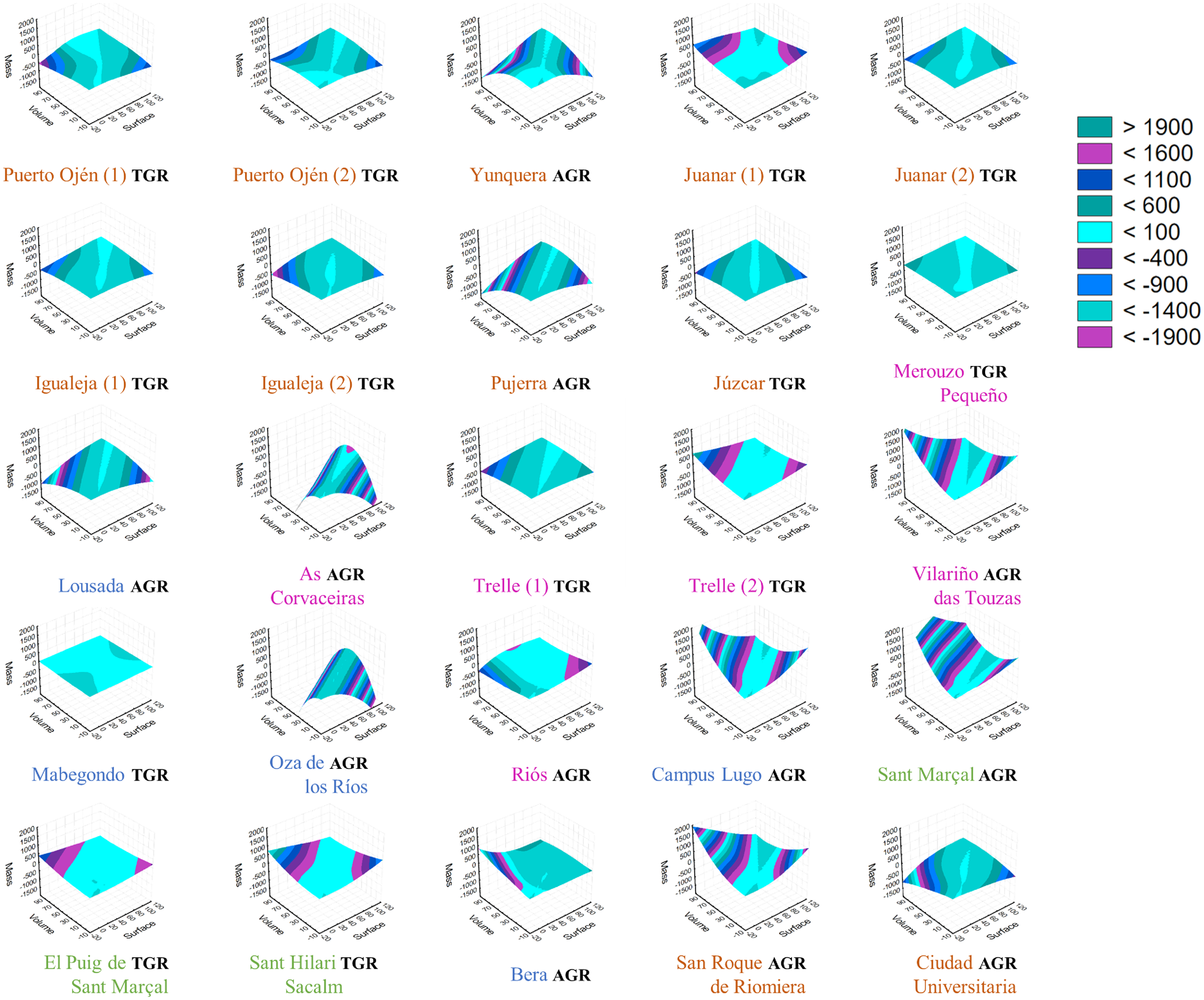
Figure 2. Surface plots of gall responses per locality. In each sampling point figure, the x-axis is the surface area; the y-axis is the volume and the z-axis is the mass. The colour of each sampling point name is related to the bioclimatic region to which it belongs according to fig. 3b. Legend values and colours are related to the measure of the variation of each plane formed by the three variables and indicate the type of gall response. Less variation in the plane and mild convexity or concavity are related to a TGR, and high variation in the plane and high convexity, concavity or intermediate curvature, appearing as sigmoidal planes, are related to an AGR. These two categories appear above each sampling point name depending on the corresponding gall response (see table 1).
SIMPROF cluster analysis based on geographical attributes shows three main groups, including all galls from the southern sampling points in a single set (South region); all galls from the northwest areas together; and a group with galls from the remaining localities (Northeast and Central regions) (fig. 3a). The last group can be further divided into two groups, but they remain united in the subsequent analyses for simplification. SIMPROF analysis of climatic variables among the sampling points shows four main groups. The significant groups (P < 0.05) reflect well the climatic classification of the sampling points (Köppen-Geiger IP regions: M-Csa/Bsk, M-Cfa/Cfb, E-Cfa/Cfb and M-Csb) (fig. 3b).

Figure 3. Dendrogram obtained from the SIMPROF cluster analyses of Iberian sampling points. (a) Similarity among points based on geographical independent variables. (b) Similarity among points based on bioclimatic independent variables.
The SIMPROF cluster analysis based on gall morphological variables (fig. 4) shows the classification of sampling points reflecting the mass and volume of galls, highlighting three significantly different groups (P < 0.05) (large-, medium- and small-sized galls, with the last group including very small galls). Large galls are associated with southern sampling points and with TGR galls, while small galls only occur at northern sampling points. However, galls from a locality of the Northwest region (Merouzo Pequeño, fig. 1a, 10) belong to the large size group, and galls from different regions are included in the medium size group.

Figure 4. Dendrogram obtained from the SIMPROF cluster analyses of Iberian sampling points considering the morphological variables of D. kuriphilus galls. (a) Similarity among points based on morphological variables based on the bioclimatic groups of fig. 2. (b) Similarity to dependent variables based on the geographic groups in fig. 2.
Kruskal–Wallis tests show that there are significant differences between the climatic and geographical regions for all the gall morphological variables (climatic, mass: H = 71.488, P < 0. 0001, volume: H = 44.058, P < 0.0001; geographical, mass: H = 66.633, P < 0.0001, volume: H = 43.481, P < 0.0001) (figs 5 and 6). These analyses show that galls are larger and with more mass in the M-Csa/Bsk (and Southern) region. Mann–Whitney U test comparisons by groups indicate that in most cases, there are differences between the South area and the other geographical regions and between M-Csa/Bsk and the other climatic regions.

Figure 5. Graphs showing the mean ± standard error of gall mass (a) and volume (b) across climatic regions, together with the results of the Kruskal–Wallis and Mann–Whitney U by groups. Different letters refer to significant paired differences.

Figure 6. Graphs showing the mean ± standard error of gall mass (a) and volume (b) across geographical regions, together with the results of the Kruskal–Wallis and Mann–Whitney U by groups. Different letters refer to significant paired differences.
The results of the GLMs (table 2) show that the most important explanatory variable of the geographic model is latitude, and for the mass and volume, this variable explains the greatest amount of their variance (39.24 and 34.72%, respectively). The most important explanatory variable of the climatic model is BIO1 (annual mean temperature), which explains 40.60% of the observed variance in mass. The pure geographical effect for mass and volume is null, and the pure bioclimatic effect is very small (1.41% for mass and 2.58% for volume). However, the combined effect for the geographical and bioclimatic models reaches 30–40% of the total variance (39.20% for mass and 32.14% to volume).
Table 2. Results of GLMs between the dependent variables (mass and volume of D. kuriphilus galls) and independent variables (geographic and bioclimatic), according to each model type

The names of climatic variables are referred to the name of Worldclim variables, accessible at https://www.worldclim.org/bioclim. These results show the explained variance of each dependent variable, its respective significance value (P = *<0.05; **<0.01; ***<0.001) and whether its effect is positive or negative with respect to the dependent variable.
All the contour plots based on the effects of the explanatory variables on gall morphological variables (fig. 7) show a similar pattern: if BIO1 is high and latitude is low (or vice versa), then gall mass and volume increase. The mass/volume relationship for the galls of the four different zones is calculated, and the slopes for these four regions are compared with the average mass/volume slope for all galls pooled together. All slopes are similar with the exception of the slope for the M-Csb galls from the North IP, which is higher (slope mean: 12.668; M-Csa/Bsk slope = 12.620; M-Cfa/Cfb slope = 12.630; E-Cfa/Cfb slope = 12.687; M-Csb slope = 15.750); therefore, gall mass increases much more than the volume in this region.

Figure 7. Contour plots showing the distribution of D. kuriphilus gall morphology (z-axis) in relation to the mean temperature (BIO1) (y-axis) and latitude (x-axis). (a) Mass and (b) volume. Values of independent variables have been standardized.
Discussion
Variation in gall morphology across the Iberian Peninsula
We found significant morphological differences in gall morphology among different sampling points (figs 2 and 4–6). Chestnut tree species respond to different environmental conditions with different morphologies (Wang et al., Reference Wang, Bauerle and Mudder2006) and physiologies (Lauteri et al., Reference Lauteri, Scartazza, Guido and Brugnoli1997), depending on light acclimation and photosynthetic capacity, and southern galls may be larger than most of the other samples because of the high production of chestnut trees at this latitude, where they are under very favourable conditions. Indeed, although the suitable niche of C. sativa is related to high rainfall and rare drought (as found on the northern IP), the photosynthetic activity of these chestnuts may be higher due to the periods of high radiation that are typical of the southern IP. Considering that C. sativa trees are distributed in the South IP in M-Csa/Bsk only at high-altitude locations as suitable sites for their cultivation, the ideal conditions of rainfall and humidity are met, and chestnut trees can grow optimally with an addition of high photosynthetic activity. This argument coincides with the observed response in fig. 7, being the larger galls at lower latitudes in warmer areas. In other parts of the chestnut distribution on the IP, particularly in the North, rainfall is abundant, and the average yearly temperature and insolation are lower (AEMET, 2014), could lead to lower chestnut tree productivity and, consequently, to relative smaller galls of D. kuriphilus (fig. 6). This fact could suggest a general correlation between plant productivity and gall size in cynipids, a hypothesis that may be tested in future analyses of other species and regions.
In the northern areas, smaller galls would more likely be aborted and the larvae die due to frost damage. For example, the galls from As Corvaceiras and Oza de los Rios (fig. 1a, 11 and 17) are small possibly because these localities have suffered periods of frost and freezing of bud trees. In January 2017, there was a period of heavy frost on the Northwest IP (AEMET, 2017), coinciding with the beginning of the period of stagnation and plant dormancy (Reale et al., Reference Reale, Tedeschini, Rondoni, Ricci, Bin, Frenguelli and Ferranti2016). It is possible that frosts are a limiting factor (and a larval mortality factor) affecting the size and mass of D. kuriphilus galls. In a premature stage of cecidogenesis, galls seem to be less effective as environment insulators for larvae (Price et al., Reference Price, Fernandes and Waring1987).
However, large galls were also found to a lesser extent in the northern samples. Considering the possible limiting effect of frosts and low temperatures on D. kuriphilus gall development and viability, only larger galls may survive under these conditions, leading to the possibility that gall size is not only a response constrained by climate (i.e. southern conditions favour larger galls) but also results from an attempt to adapt to colder environments (i.e. in the North). This is related to the microenvironment hypothesis of the adaptive significance of galls (Price et al., Reference Price, Fernandes and Waring1987; Stone et al., Reference Stone, Schönrogge, Atkinson, Bellido and Pujade-Villar2002), although the adaptation of these structures also responds to other factors, such as the global environment. This finding could support the ‘microenvironment hypothesis’ (Price et al., Reference Price, Fernandes and Waring1987; Stone et al., Reference Stone, Schönrogge, Atkinson, Bellido and Pujade-Villar2002), with the frosting regime as a natural selection driver for D. kuriphilus. In support of this hypothesis, the slopes of the mass/volume relationships across the galls of the four different zones were similar, except for the M-Csb galls from the North. The reason for this different mass/volume relationship could be the Csb climate conditions (Kottek et al., Reference Kottek, Grieser, Beck, Rudolf and Rubel2006) at high latitudes, which are rainy and cold but also present greater continentality and less isothermality, leading to both droughts and frosts in the region.
Results indicate that there are differences in gall morphology among sampling points throughout the IP (figs 4–6). Up to 30–40% of this variance was explained by geographic and climatic variables, particularly by their combination (table 2). As most of the variance remains unexplained, there must be other unknown factors acting on gall morphology, such as differences between chestnut tree varieties, tree age, the years of settlement of the pest in the area, tree aggregation, the population density of D. kuriphilus (Bonsignore and Bernardo, Reference Bonsignore and Bernardo2018) and the existence of resistant ecotypes (Nugnes et al., Reference Nugnes, Gualtieri, Bonsignore, Parillo, Annarumma, Griffo and Bernardo2018). Gall size also depends on the number of eggs laid within the chestnut bud (Panzavolta et al., Reference Panzavolta, Bracalini, Croci, Campani, Bartoletti, Miniati, Benedettelli and Tiberi2012, Reference Panzavolta, Bernardo, Bracalini, Cascone, Croci, Gebiola, Iodice, Tiberi and Guerrieri2013; Bernardo et al., Reference Bernardo, Iodice, Sasso, Tutore, Cascone and Guerrieri2013), and are related to the D. kuriphilus assessment period and the population density. However, in the northeast area, where D. kuriphilus was firstly introduced in the IP (2012), no galls larger than the rest of the areas were observed (figs 4 and 6). Also, concerning the south and northwest areas, D. kuriphilus was introduced in the same year (2014) and the two areas present dissimilar gall sizes (fig. 6) and that provides the observed relationship between gall size, mean temperature and latitude (fig. 7). Furthermore, microclimatic variables may influence gall size and may therefore explain why some points located very close to each other (e.g. Juanar (1) and Juanar (2), separated by 1 km) harboured galls of different sizes.
As D. kuriphilus is an alien species in a foreign territory, it is possible that it is not fully adapted to the conditions of this environment, where it may be found in less optimal areas than in the heart area of its original distribution. Considering niche-based potential models for D. kuriphilus on the IP (Gil-Tapetado et al., Reference Gil-Tapetado, Gómez, Cabrero-Sañudo and Nieves-Aldrey2018), some of the locations studied here, such as As Corvaceiras and Oza de los Rios (fig. 1a, 11 and 17), are not as suitable as other nearby chestnut forest areas, which may result in an AGR at these sampling points (fig. 2). In fact, suitability data (Gil-Tapetado et al., Reference Gil-Tapetado, Gómez, Cabrero-Sañudo and Nieves-Aldrey2018) and the gall response categories appeared to be associated (R 2 = 0.311; P = 0.004), and significant differences were observed between groups (Kruskal–Wallis test: KW-H = 5.097; P = 0.024; and simple regression: r 2 = 0.311; P = 0.004). Similar results were obtained when using the suitability of the zones near the sampling locations within a buffer of 10 km (Kruskal–Wallis test: KW-H = 5.861; P = 0.002; and simple regression: r 2 = −0.498; P = 0.011). It is possible that chestnut trees in low-suitability areas induce a different, variable gall response (fig. 2), related to lower production, lower resource availability or even lower fitness of Castanea trees. Because the D. kuriphilus distribution on the IP is related to human activities (i.e. transport of tree seedlings; Avtzis et al., Reference Avtzis, Melika, Matošević and Coyle2019), it is possible that it occurs in suboptimal areas regardless of the presence of chestnut forests (Gil-Tapetado et al., Reference Gil-Tapetado, Gómez, Cabrero-Sañudo and Nieves-Aldrey2018).
Possible consequences of gall morphology variability for the communities of D. kuriphilus parasitoids
In its invaded areas, D. kuriphilus has recruited native parasitoids (Askew et al., Reference Askew, Melika, Pujade-Villar, Schonrogge, Stone and Nieves-Aldrey2013; Cooper and Rieske, Reference Cooper and Rieske2007; Aebi et al., Reference Aebi, Schönrogge, Melika, Quacchia, Alma and Stone2007; Quacchia et al., Reference Quacchia, Ferracini, Nicholls, Piazza, Saladini, Tota, Melika and Alma2012; Matošević and Melika, Reference Matošević and Melika2013; Kos et al., Reference Kos, Kriston and Melika2015; Jara-Chiquito et al., Reference Jara-Chiquito, Heras and Pujade-Villar2016; Nugnes et al., Reference Nugnes, Gualtieri, Bonsignore, Parillo, Annarumma, Griffo and Bernardo2018). It would be particularly interesting to compare the northwestern and southern IP parasitoid communities associated with D. kuriphilus since this cynipid arrived in these areas in the same year (2014). In general, all known parasitoids recruited by this cynipid exhibit a wide host range (Aebi et al., Reference Aebi, Schonrogge, Melika, Alma, Bosio, Quacchia, Picciau, Abe, Moriya, Yara, Seljak, Stone, Ozaki, Yukwa, Ohgushi and Price2006; Quacchia et al., Reference Quacchia, Ferracini, Nicholls, Piazza, Saladini, Tota, Melika and Alma2012). However, their abundance, richness and community composition can vary in different areas of the invaded range. This variation is related to which parasitoid species attack adjacent native oak cynipid communities (Aebi et al., Reference Aebi, Schonrogge, Melika, Alma, Bosio, Quacchia, Picciau, Abe, Moriya, Yara, Seljak, Stone, Ozaki, Yukwa, Ohgushi and Price2006, Reference Aebi, Schönrogge, Melika, Quacchia, Alma and Stone2007). As parasitoid species discriminate among galls of different morphologies during host and oviposition site selection (Weseloh, Reference Weseloh, Norlund, Jones and Lewis1981; Vinson, Reference Vinson, Kerkut and Gilbert1985, Reference Vinson and Gupta1988; Vet and Dicke, Reference Vet and Dicke1992; Quicke, Reference Quicke1997), at least some of these species may either intentionally choose D. kuriphilus galls or be confused by them and mistake them for native cynipid galls in the case of morphological similarity. European native galls with a similar morphology to those of D. kuriphilus are produced by Plagiotrochus australis (Mayr, 1882), Plagiotrochus quercusilicis (Fabricius, 1798), Andricus curvator (Hartig, 1840), Biorhiza pallida (Olivier, 1791) or the sexual generation of Neuroterus quercusbaccarum (Linnaeus, 1758) (Nieves-Aldrey, Reference Nieves-Aldrey2001). These galls of native species have been the target of studies of host preference of Torymus sinensis Kamijo, 1982, which is commonly used as a chestnut gall wasp biocontrol agent in other invaded countries (Moriya et al., Reference Moriya, Shiga and Adachi2003; Quacchia et al., Reference Quacchia, Moriya, Bosio, Scapin and Alma2008, Reference Quacchia, Moriya, Askew and Schönrogge2013; Matošević et al., Reference Matošević, Lacković, Melika, Kos, Franić, Kriston, Bozso, Seljak and Rot2016; Paparella et al., Reference Paparella, Ferracini, Portaluri, Manzo and Alma2016; Avtzis et al., Reference Avtzis, Melika, Matošević and Coyle2019). In these host preference studies (Ferracini et al., Reference Ferracini, Ferrari, Pontini, Nova, Saladini and Alma2017, Reference Ferracini, Bertolino, Bernardo, Bonsignore, Faccoli, Ferrari and Rocco2018), authors obtained that this natural enemy can oviposit in these galls, although the chestnut gall wasp remains its preferred host. Considering this, as T. sinensis is a fairly specialized species synchronized with D. kuriphilus, generalist native parasitoids would be more likely to parasitize this new resource in chestnuts.
The parasitoid recruitment rate per area could depend on the morphology or growing stage of D. kuriphilus galls, which is in turn dependent on environmental conditions (Bonsignore and Bernardo, Reference Bonsignore and Bernardo2018; Gil-Tapetado et al., Reference Gil-Tapetado, Gómez, Cabrero-Sañudo and Nieves-Aldrey2018; Panzavolta et al., Reference Panzavolta, Croci, Bracalini, Melika, Benedettelli, Tellini and Tiberi2018; Bonsignore et al., Reference Bonsignore, Vono and Bernardo2019). In addition, the influence of size and shape of host has been previously observed in other parasitoid–host relationships (Jones, Reference Jones1983; Stone et al., Reference Stone, Schönrogge, Atkinson, Bellido and Pujade-Villar2002; Bonsignore and Bernardo, Reference Bonsignore and Bernardo2018). Bonsignore and Bernardo (Reference Bonsignore and Bernardo2018) conclude that parasitoids seem to prefer small D. kuriphilus galls (i.e. easier to parasitize galls by having a thinner wall, Cooper and Rieske (Reference Cooper and Rieske2010)). Areas with an AGR (fig. 2) may harbour a parasitoid community with higher richness and diversity, which may result in higher recruitment compared with areas with a TGR, which produces larger galls. Despite this, community composition of native oak gall wasp parasitoids and the degree of synchronization of these species with their host phenology may be factors to consider (Bonsignore et al., Reference Bonsignore, Vono and Bernardo2019). As an example of this interaction, the synchronization of parasitoids that are specialized with an early development stage of the gall can be influenced by the temperature, that cause a sooner or later develop of the chestnut tree buds and the consequent formation of galls in their more conspicuous stages.
The results of our study emphasize other previously published articles about the effect of temperature on D. kuriphilus growth and phenology in an invaded territory, modifying the morphological characteristics of the galls and probably influencing their interaction with the native parasitoids and biological control.
Supplementary material
The supplementary material for this article can be found at https://doi.org/10.1017/S0007485320000450.
Acknowledgements
This study was financed by an Encomienda de Gestión from MAPAMA to Agencia Estatal CSIC, 16MNES003, awarded to JLNA, DGT, JF Gómez and CP, and by project AGL2016-76262-R (AEI/FEDER, UE), awarded to JLNA. We would like to thank Maria Pilar Rodriguez, Carmen Rey and Jose Ignacio (Chechu) Aguirre for help with collecting galls and the sampling work.
Author contribution
Conceived and designed the work: DGT, FJCS, JFG and JLNA. Performed the experiments and analysed the data: DGT, FJCS and CP. Contributed materials/analysis tools: DGT, FJCS and JLNA. Wrote the paper: DGT, FJCS, JFG, CP and JLNA.
Financial support
This study was financed by an Encomienda de Gestión from MAPAMA to Agencia Estatal CSIC, 16MNES003 awarded to JLNA, DGT, JFG and CP.
Conflict of interest
The authors have declared that no competing interests exist.


