1. Introduction
Financial firms are regularly asked to provide reassurance that they have the capital strength to cope with the events of the future. Regulators, shareholders, market counterparties and individual policyholders alike demand assurance that capital buffers are large enough to withstand potential losses. Where a track record of prudent management might have sufficed to engender trust in the past, firms are now asked to report, or are keen to demonstrate, their supposed strength in a quantitative manner. The “1-in-200 year” test in Individual Capital Assessment and Solvency II calculations are examples of quantitative demonstration of capital strength in insurance that echoes the 5% daily value-at-risk (VaR) number monitored by banks. Section 1.1 contains examples of two published cases where the capital calculations based on 1-year VaR of firms proved to be insufficient.
Practitioners involved in these calculations are aware that a purely mechanical approach to a capital or solvency calculation can be unhelpful. This paper looks at the various reasons why a purely mechanical approach may not be possible or justified. It also presents tools and techniques to help address some of these difficulties.
The main reasons for this, which are behind much of the thinking in this paper, can be summarised in terms of breadth and depth:
Too much breadth – although unintuitive at first sight, one of the biggest issues related to the calculation of solvency capital is that a glut of data/information on the numerous potential risks that a firm is exposed to may actually make it difficult to see the wood from the trees. In other words, a good understanding of what risks are important to the business is increasingly necessary, and a simplification or sifting stage is essential to begin to quantify the risks faced by the firm.
Insufficient depth – to adequately calibrate a probability event in the tail of a distribution requires a large amount of data, which is often simply not available. There may not even be enough data to know what model is most suitable for these tail events, never mind what parameters should be chosen for this model.
In both cases, judgement is needed to make sensible choices, but these choices will influence the results. Understanding this influence, and modifying results to allow for it, should be an important aspect of capital calculations. This paper seeks both to offer a guide to the kinds of things that can go wrong and to provide a set of tools that can be used to make capital calculations more robust.
It is tempting to believe that complex analytical and statistical approaches are doomed to fail and that a simple approach is the best way forward. Haldane (Reference Haldane2012) makes an erudite argument for such an approach, and we recommend it as further reading. Our view is that risk models are necessary but have to be carefully built, given that they can at best be an approximate representation of the real world. In particular, practitioners need to be aware of the impact of the multitude of choices they are forced to make, and model results should be treated with a healthy dose of wariness.
1.1. A (Hypothetical) Motivating Example
We consider a set of hypothetical but not implausible events for a financial firm that assesses at the start of the year that €10 bn is sufficient to absorb losses with 99.5% probability. By the end of the year, the firm has lost €20 bn. Many things have gone wrong at once, including the following:
Accounting change
• A clarification in the regulatory calculation of the illiquidity premium meant that the insurer could no longer use the yield on certain illiquid assets to discount the liabilities. The liabilities rose as a result of this change, leading to an accounting loss. At the same time, a change in tax rules meant that a deferred tax asset previously considered recoverable had to be written off.
Unmodelled heterogeneity
• A problem arose with a set of policies that, for calculation convenience, had been modelled together. It turned out that within a group of policies assumed to be homogenous, there was in fact a variety of investment choices; as a result, a large block of these policies had guarantees that were significantly into the money. Policyholders selectively took advantage of these guarantees, producing costs far beyond those projected from the capital model.
Market risks
• New risks emerged that had not previously been modelled explicitly. Specifically, a loss on derivative positions arose from the widening of spreads between swaps based on LIBOR and overnight index swaps. A euro government defaulted on its bonds.
• A change in the shape of the credit spread curve meant that the existing market-consistent ESG could not exactly calibrate the year-end market conditions. Concerned about how this would appear in upcoming meetings with the regulator, a new ESG from a different provider was put in place at short notice. However, for reasons that are still not fully transparent, this led to an increase in the stated time value of liability options.
Non-market risks
• Losses from an earthquake in the Middle East were substantially greater than the maximum possible loss calculated from a third-party expert model. The reasons for this seem to be a combination of a disproportionate number of January policy inceptions (the model assumed uniformity over the year), inadequate coverage of the region in the external catastrophe model, and poor claims management exacerbated by political instability and corruption.
• The annuity portfolio took a one-off hit because of a misestimation of the proportion married and a strengthening of the mortality improvement rates.
Poor returns on new investments
• Early in the year, the firm participated in some securitised AAA investments that exploited market anomalies to provide yields closer to those on junk bonds. The capital model had been based on the portfolio before this participation. The participation turned out to be disastrous, and virtually all the investment had to be written off following an avalanche of unforeseen defaults in the underlying assets.
Legal loophole
• Many life insurance claims became due following an industrial accident. The insurer was confident that a proportion would be recovered from reinsurers as assumed within the capital model. However, the reinsurance contract contained a clause not captured in the capital model, which limited payouts in the event of large losses from a single event.
Although our example in this case is hypothetical, there are indeed real examples of firms who proclaimed that they held economic capital to withstand a loss equivalent to a very extreme event (e.g. a 1-in-2,000 year) before losing a multiple of that amount of that figure.
Table 1 shows the published 1-year VaR figures for two of the well-publicised cases in 2008 that ultimately led to state bailouts – AIG (2008) and Fortis (2008). We have also calculated the confidence level associated with the experienced losses, assuming normal distributions.
Table 1 Published 2008 1-year VaR for AIG and Fortis

1Based on the upper value of $19.5 bn ECAP.
It is of course theoretically possible that such an outcome was a case of exceptionally bad luck, but with hindsight we have seen how risks that ultimately proved to be important were either overlooked or scoped out of the capital models.
1.2. Capital Model Scope
Our hypothetical example in section 1.1 highlights many possible sources of loss. Whereas some of these are avoidable, and others may be captured within a stochastic internal model, many will not be modelled. These losses may be attributed to lack of knowledge and genuine model uncertainty rather than an explicit stochastic element. It is debatable whether probability theory is the right tool to address such risks.
If these risks are simply ignored, then firms are likely to see frequent exceptions, that is, experience losses worse than the previously claimed 1-in-200 event. Mounting evidence of such exceptions could undermine a firm's claims of financial strength, and may even call into question the advertised degree of protection (e.g. 1-in-200) that a supervisory regime claims to offer.
Thus, rather than simply asserting (ex post) that these risks were out of scope, it is therefore desirable that risks are identified and some attempt is made at quantification, even if a variety of techniques are needed to address different elements.
1.3. What's in this Paper?
In the remainder of this paper, we focus on four specific types of error and also examine some broad themes.
Section 2 considers the overall aspect of choice or judgement with respect to modelling, explaining the basic need for judgement, and highlighting several broad areas where judgement/choice is manifested in the context of actuarial modelling. The chapter then considers each area, and introduces some methods of mitigating the need for judgement as well, providing some observations on good practice for cases where judgement is inevitable.
Section 3 looks at the choice of risks to include in a model. Two key aspects are considered. These are the selection of features and extraction of features to be modelled. How to allow for the risks not explicitly covered in the model is also discussed. Some mitigants including grossing-up techniques and stress testing are discussed.
Section 4 looks into model and parameter risk and describes classic statistical approaches to parameter error, showing constructions of confidence and prediction intervals, incorporating the T-effect, for a range of distributions and data sample sizes. It also tackles model error, with a number of examples, before discussing some techniques to assess model errors.
Section 5 looks at several aspects of errors introduced by calculation approximations when, in the interest of faster run times, assets or liabilities are approximated by polynomials. This first looks at proxy models, and the potential errors that they introduce, as well as the errors introduced by Monte Carlo sampling.
Section 6 includes a summary of key conclusions from previous sections, our concluding thoughts on the topic and references.
Appendix A draws together the use of Bayesian methods in risk analysis, including the application of judgement, Bayesian networks and the use of Markov chain Monte Carlo methods to compute posterior distributions.
Appendix B gives details of the liability valuation formulas used in the proxy model examples from section 5.
2. Judgement
First, it is important to acknowledge that judgement is a necessary and inescapable part of actuarial modelling, and it is very difficult (in fact, one could argue impossible with the exception of pathological examples) to simply avoid the need to make any choices. Moreover, as we shall explain, judgement permeates almost every aspect of modelling, which means that one may encounter the need to make choices at various levels.
Another aspect is that any judgement, by definition, depends to a certain extent on who is making the judgement, and the framework within which they need to make the judgement. In the United Kingdom, the board is ultimately responsible for all assumptions and judgements, and statutory audits in the United Kingdom assert that a set of accounts provide a “true and fair” view, in accordance with the accounting principles.
A specific element of the audit assesses whether judgements made by management during the production of a set of “true and fair” accounts are reasonable. A reasonable judgement may be interpreted as within the range of conclusions an expert could draw from the available data, and will have regard to common practice in the market. The range for reasonable judgements may be narrower than parameter standard errors in a statistical sense, especially when data are limited.
An audit process also looks for errors that are unintentional human mistakes, such as the use of an incorrect tax formula or omitting an expense provision. Any such mistake is assessed using the concept of a “materiality” limit. This is an amount of error, expressed in currency terms, which is deemed not likely to change the decisions of the users. Material errors should be corrected, but a clean audit can still be granted provided the aggregate effect of mistakes is within the materiality limit.
The exercise of judgement is not a mistake; it is possible for two reasonable judgements to differ by more than the materiality limit. Therefore, decision makers relying on financial statements should be aware that alternative judgements in the account preparations could have led to different decisions. True and fair accounts must be free of material mistakes but cannot be free of material judgement.
Thus, there is a considerable element of judgement embedded in the production of the basic “realistic” or “best estimate” balance sheet, even before extrapolating into the calculation of the capital required to withstand a hypothetical 1-in-200 event.
We try to address this aspect of judgement by looking at two elements:
• Section 2.1 aims to broadly categorise the different manifestation of choice/judgement inherent within modelling, and point the reader to tools that potentially deal with each aspect.
• It is extremely unlikely that we can do away with judgement altogether, and there will be aspects that inevitably require judgement. In section 2.2, we try and summarise some good principles within current industry practices.
2.1. Manifestations of Judgement
Judgements are an integral part of any modelling exercise, because any model is necessarily a simplified representation of the real world and as such needs to be stripped down to its most relevant components. This ensures that the model is a useful analogy of the real world for the specific purpose that a model is required for. The process of stripping down to the bare useful components and “calibrating” the resultant model inevitably has a large amount of judgement associated with it. In the limited context of actuarial modelling, this judgement can broadly be thought to manifest itself in the following ways:
• choosing which risk factors to model;
• choice of overall model framework;
• choosing individual parts of the model;
• choice of calibration methodology;
• judgements inherent within the data itself;
• choice of parameters.
One can imagine that these have (broadly) decreasing levels of significance to the end results. However, the industry appears to have the greatest focus on the final (and perhaps second to last) elements of parameter choice and calibration methodology, often to the detriment of the overall choice of framework and model fitting. For example, companies may focus most of the documentation and rationale of expert judgement in the final two categories, potentially at the expense of reduced oversight and attention paid to the substantial implied judgements involved in the first two categories.
2.1.1. What Risk Factors to Model?
Perhaps the single biggest modelling choice to be made by a company is simply what risks to model. As briefly explained above, a model can only hope to be a simplified representation of the reality it intends to model. A philosophical way of thinking about it is that any model of the universe needs to be at least as large as the universe itself, and in fact in order for us to project it into the future faster than real time, it needs to be even larger.
A key constraint on the number of risk factors to include in a model is availability of resources. Human resources, computer resources and time are required in most modelling exercises and these have to be used in the most efficient manner. To that end, we need to choose the most appropriate aspects to model. Suppose we could simplify the modelling problem considerably, by converting the problem into a simple choice regarding the number of “risk factors” to model. It can be shown that the number of modelling choices faced by a company is simply enormous! For example, section 3.1 details a case study to highlight the enormity of this decision, where over a million inputs to the balance sheet are summarised by as few as 100 risk factors.
Needless to say, choosing the risk factors to model is an extremely important exercise and one that should not be taken lightly. Also important is that once the modelling choices have been made is how to allow for the risk factors that are not modelled. This is addressed in the “grossing-up techniques” commentary in section 3.3.
2.1.2. Choice of Overall Framework
This is quite possibly the second most significant judgement to be made within a (capital) modelling context, although it is not always appreciated as such. Of course, the materiality of the different choices depends on the particular problem at hand. We try to illustrate this in the context of aggregation methodology using a very simple case study with two risks (described as two products of equal size, A and B):
• Each risk akin to a simple product with a guaranteed £100 m liability, in which not all the risks are hedgeable. There is a residual 1-in-200 risk that the assets (and capital) would lose half their value. The extra capital required at time 0 such that the product has a 99.5% probability of meeting its guarantees at time 1 is (an extra) £200 m (£100 m for each product).
• The two products are assumed to be uncorrelated.
Let us now consider two commonly used methods of calculating the aggregate capital requirement:
1. Using an “external correlation matrix” approach, the answer is relatively simple. The aggregate capital requirement can be calculated as
 $$$\sqrt {Capital_{A}^{2} + Capital_{B}^{2} } $$$
, which is £141.6 m in total and £70.8 m per product.
$$$\sqrt {Capital_{A}^{2} + Capital_{B}^{2} } $$$
, which is £141.6 m in total and £70.8 m per product.2. Using an alternative approach of undertaking a Monte Carlo simulation of the losses of the two products assuming the distribution of the losses are lognormal (again, a popular choice amongst practitioners) with the same 1-in-200 individual capital requirements. This produces a different aggregate capital requirement of £121 m and £60.5 m post-diversification capital requirement for each product.

This simple example of the impact of the choice of the aggregation framework shows that the aggregate capital requirement can differ by 20% of the liabilities. This example is not special in any sense, in that the two products could represent pretty much any two risk factors.
One can appreciate that there are multiple choices to be made in simply aggregating different risk factors. This is further compounded by choices that need to be made in relation to exotic copula structures, non-linearities, etc.
Finally, this example only touches on a very specific aspect of framework choice; there are many other implicit judgements necessitated by trying to create a simplified representation of the real world. There is a long list of other judgements that need to be made, examples of which include:
• using heavy models versus lite (proxy) models;
• if proxy model, choice of proxy model;
• what measure is used to estimate capital, for example, VaR, tail VaR, etc;
• granularity of assets, model points;
• use of instantaneous stress approximation (time 0, time 1 or other);
• holistic model of the business versus detailed product-specific models aggregated;
• treatment of new business;
• fungibility of capital;
• measure of correlation used.
2.1.3. Choice of Model Components
The choice of model for each risk is an important aspect of modelling. A previous paper, an extract of which is showed below, from this working party (Frankland et al., Reference Frankland, Smith, Wilkins, Varnell, Holtham, Bifis, Eshun and Dullaway2009) showed that fitting different models to the same historical data can have a range of different results, even when using relatively large amounts of data (Chart 1).
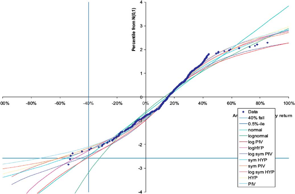
Chart 1 Quantile-Quantile plot of UK equity returns, 1969–2008, with various fitted models
“Even after settling on a single data set, the fitted curves for U.K. produce a wide range of values for the 1-in-200 fall. The most extreme results are from a Pearson Type IV, applied to simple returns, which implies a fall of 75% at the 1-in-200 probability level. At the other extreme is the lognormal distribution, with a fit implying that even a 35% fall would be more extreme than the 1-in-200 event. Other distributions produce intermediate results”.
Chart 2 shows the 0.5th percentile estimated using different models for the UK and Denmark. Interestingly, the same extreme potential model error is also true for Denmark (which also has relatively large amounts of historical data), but in this case the models that result in the most and least extreme values are completely different.
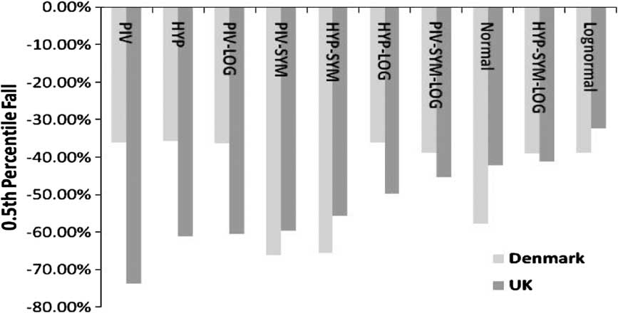
Chart 2 0.5th percentile estimated using different models based on UK and Danish equity data
Another example of model risk is described in section 4.2 and the reader is also referred to a recent paper by Richards, Currie and Ritchie, and the subsequent discussion.
2.1.4. Choices Inherent within the Calibration
There are other, more commonly acknowledged calibration choices that should be noted in the same context. For example, calibration of a model is required to fit historical data to a 1-in-200 event, and one of the decisions is the choice of data period to use. Very simply, if we are using x years of data, then the model would accept the worst event within this data window as being a 1 in x event. Thus, the choice of data window makes an important contribution to the results, and it is important to note that even picking any available data set comes with a default assumption regarding the data period.
This context results in an obvious place where one may want to exercise judgement, that is, one may want to impose some views on the extremity of actual events observed. An obvious example can be constructed by using very short data series that included the recent credit crisis, which would naively overestimate the resulting extreme percentile calculated by assuming such an extreme event that would occur regularly within such a short time period. Of course, it goes without saying that the reverse would also have been true when looking at short-term data before the recent financial crisis.
Another example of judgement related to calibration is the choice of method to estimate the parameters of a model. The two approaches that are commonly used are maximum likelihood estimation and the method of moments (described further in section 4.1.4). In calibration exercises where data are limited, these different approaches can lead to very different results.
2.1.5. Judgement Inherent within Underlying Data
Before the application of judgement to the data, it is useful to consider the nature of the raw data used to calibrate the model. The data might not themselves be accurate, being based on estimates, or might contain a systemic effect that would influence our interpretation of the data and perhaps the calibration.
A recent example of data that is based on estimates, which was perhaps not generally appreciated at the time, is the ONS mortality data for older ages in England and Wales. The results of the 2011 Census revealed that there were 30,000 fewer lives aged 90 years and above than expected. In absolute terms, a difference of 30,000 lives is not a large change. However, in relative terms, it represents a reduction of around 15%. Between census years, the exposure to risk is an estimated figure. The funnel of doubt around the estimate increases as the time since the last census increases. The ONS data, being based on a large credible data set, are the source of most actuarial work on longevity improvements, including the projection model developed by the continuous mortality investigation. One implication of the recent census data is that estimates of the rate of improvement of mortality at high ages might have been significantly overstated.
An example of a systematic effect that may be present in data, and should be considered before using any data to calibrate an internal model, would be the derivation process behind a complex market index. As an illustration, Markit publishes a report on its iBoxx EUR Benchmark IndexFootnote 1 that documents multiple changes to the basis of preparation. This index may be considered a suitable starting point to construct a model of future EUR bond spread behaviour, but such an analysis should consider the effect of the various changes. Of course, the report from Markit contains extensive details of the past index changes, but an equivalent level of detail might not be available for other potential data sources.
2.1.6. Choice of Parameters and Expert Overlay
Irrespective of the model we have chosen to use, we would need to supply it with suitable parameters. This can be done by using some statistical methods of choosing the best parameters, acknowledging the parameter uncertainty inherent from fitting to limited data. Section 4.1.1 looks at possible ways of quantifying the risk capital where parameters are uncertain.
In addition to genuine parameter uncertainty (assuming that past data are truly reflective of the future), we may also have uncertainty as the future conditions may be different to historic conditions (taking interest rates, for example). In this case, management still needs to make some judgements on the choice of parameters.
This judgement on model parameters can be explicit or implicit. For example, at the most explicit level, one may override the 1-in-200 stress itself by superimposing the views of investment experts. In many cases, the paucity of data and the changing economic landscape makes this a regular part of the capital calculation exercise. Alternatively, judgement can be more implicit in the structure of the model. For example, conditional on the form of the model, one may have prior views on certain parameters (e.g. we may have a prior view on the volatility parameter of a lognormal distribution).
However, it should be recognised that any judgement (even though necessitated because of poor data and changing environment) is ultimately subjective. One advantage of explicit judgement (over implicit judgement) is that it is extremely transparent and openly recognises that models and data can only go so far in terms of predicting future distributions.
For either explicit or implicit judgement, we need to recognise that, although one may have a better base assumption, parameter uncertainty (section 4.1.1) still needs to be taken into account. In addition, one should aim to follow a good process when coming up with the parameters, and some observations on current practice within the industry are discussed in the next section.
2.2. Expert Judgement: Current Practices
Judgement is by no means limited to actuarial modelling, and it has been the subject of much literature outside of the financial world, for example, engineering and public health. From a purely statistical viewpoint, there is much to learn from Bayesian statistics, and a summary of Bayesian methods is provided in Appendix A, which we hope the readers find useful. In addition, there has been substantial research on this subject in other fields, particularly science and engineering (see Ouchi, Reference Ouchi2004 for a literature review of expert judgement research). We refer to some examples as extremely useful reading,Footnote 2 and perhaps learning good principles on judgement from other fields could be the scope of further actuarial research.
However, perhaps because of the huge range of possible decisions to make within actuarial modelling itself, we limited our scope to discuss aspects of current practices in the UK insurance industry. It quickly becomes evident that judgement has always been a part of risk modelling, even if it has not always been explicit. More recently, as firms started to prepare for Solvency II, there has been a much greater level of codification and documentation of expert judgement, as with other aspects of modelling. In this section, we look at how insurance firms are currently approaching this area and briefly look at research on expert judgement outside financial modelling.
2.2.1. Regulatory Background
The Solvency II Directive does not contain any direct references to expert judgement, but its use is anticipated in the Level 2 technical standards:
Expert judgement
“1. Insurance and reinsurance undertakings shall choose assumptions on the issues covered by Title 1, Chapter VI of the Directive 2009/138/EC based on the expertise of persons with relevant knowledge, experience and understanding of the risks inherent in the insurance or reinsurance business thereof (expert judgement)”.
Article 4, implementing measures, states that:
“Insurance and reinsurance undertakings shall choose assumptions on [the issues covered by Title 1, Chapter VI of the Directive 2009/138/EC] [valuation of assets and liabilities, calculation of capital requirements and assessments of own funds] based on the expertise of persons with relevant knowledge, experience and understanding of the risks inherent in the insurance or reinsurance business thereof (expert judgment).
Insurance and reinsurance undertakings shall, taking due account of the principle of proportionality, ensure that internal users of the relevant assumptions are informed about its relevant content, degree of reliance and its limitations. For this purpose, service providers to whom functions have been outsourced shall be considered as internal users”.
Level 3, Guideline 55 requires that:
“The actuarial function should express an opinion on which risks should be covered by the internal model, in particular with regard to the underwriting risks. This opinion should be based on technical analysis and should reflect the experience and expert judgement of the function”.
CEIOPS issued a consultative paper on internal models (CP56) in 2009 that, inter alia, set out its views at that time on expert judgement, commencing that “CEIOPS recognises that in a great many cases expert judgement comes into play in internal model design, operation and validation”. Further references from the CP are set out in the Appendix to this policy.
It is likely that the use of expert judgement will be subject to Level 3 guidance. EIOPA prepared an early draft guidance paper on expert judgement, which concentrated on the need for proper documentation, validation and governance of assumptions derived by expert judgement. It also identified the need for clear communication between users and providers of expert judgement to avoid misunderstandings. However, with the ongoing delays to the Solvency II project, it is not clear when this particular guidance will be open to public consultation.
In a letter to firms on IMAP progress in July 2012 (Adams, Reference Adams2012), the FSA identified expert judgement as an area for additional commentary. This recognised expert judgement as important and necessary in many aspects of internal models but identified areas for improvement that include the same areas of documentation, validation and governance. This feedback indicates that firms are finding it challenging to integrate expert judgement, with its inevitable uncertainties, into internal model processes where the emphasis is on a high standard of justification and documentation.
Against this background, a wide range of practices have developed. We comment below on a few of these, based on the experience of members of the working party and a survey made by the Solvency & Capital Management Research Group (Michael et al., Reference Michael, Roger and Peter2012) covering 15 UK life firms. Our comments are biased towards risk calibration in internal models, although, as we note below, expert judgement may apply in many other areas.
2.2.2. Scope of Expert Judgement
Expert judgement can be applied in many areas of actuarial work and not limited to deciding on the distribution of risks. Examples of other areas where expert judgement is commonly used include management actions applied in extreme scenarios, asset valuation in illiquid markets and the use of approximations. Expert judgement applies to standard formula calculations and internal models. Firms differ on which areas are within the scope of expert judgement and in fact defining that scope is not straightforward. There is almost no area of a capital model that does not involve some subjective aspects, and thus it is difficult to determine where the boundary should lie.
Defining when expert judgement should be used is also not easy. Sometimes there seems to be an assumption that data analysis and expert judgement are mutually exclusive, usually with the expectation that expert judgement is used only when data are insufficient to be relied on alone. In practice, it seems more likely that decisions will combine both, but with more weight on expert judgement as the quantity or quality of data diminishes.
In the area of risk distributions, expert judgement is commonly applied to the choice of data, calibrated parameters of risk models and correlations. It is also commonly used to adjust the tails of the distribution that are not considered sufficiently extreme, or conversely, are considered too extreme.
A more fundamental divergence between firms is whether the choice of overall risk model is considered to be subject to expert judgement or not. In section 2.1, we have illustrated how model risk can be as significant as other modelling decisions, if not more so; however, as we noted above, it seems that some firms limit the scope of expert judgement to the choices made once the model is selected.
2.2.3. Expert Judgement Policies
Most firms have developed a framework for expert judgement and this is usually embodied in an expert judgement policy. This is commonly a standalone policy covering all applications of expert judgement, but may instead be embedded in the documentation of those parts of the internal model where judgement is applied. Typically, the policies cover the high-level principles and the governance process, such as the various levels of review and signoff needed for the approval of specific expert judgements. Other contents vary widely and there are some significant differences in the scope and application of expert judgement.
2.2.4. Who are the Experts?
Arguably, the single most important aspect of expert judgement is simply identifying suitable and relevant experts. Policies may indicate what criteria are used to establish whether someone qualifies as an expert, but often there is no formal process to identify them in advance. Instead the choice might be left to the modeller's discretion, which allows for some flexibility, but one may need to be careful to ensure that a wide enough range of views is sought. Another important aspect is for the experts to be sufficiently independent of both the calibration process and the capital calculation process. The importance of this is likely underestimated, as are the risks of expert judgement influencing the capital outcomes.
Occasionally more than one expert may express a view, which in turn leads to differences of opinion that need to be merged into a single modelling decision. Thus, in addition to model risk, we now have to consider “expert risk”. Some firms get round this by using a technical committee, and therefore effectively (or explicitly) the committee acts as the “expert” and the committee process resolves diverse views into a single decision. However, committees are only one way to aggregate the opinions of several experts and may not be the most effective, and this aspect has been better researched in other fields. SeeFootnote 3 Ouchi (Reference Ouchi2004) for a literature review of expert judgement research. A large part of this research covers elicitation and aggregation of expert judgement, which so far do not seem to have been widely considered in economic capital applications (other than possibly operational risk).
Elicitation is the process of gathering expert judgement. Experts are human and can be subject to various biases or herding. In a group or committee, the most senior, most confident or simply most biased (e.g. not independent) experts may overrule other opinions. Various structured approaches to elicitation have been developed to reduce the impact of these biases (Cooke & Goossens, Reference Cooke and Goossens1999) give a detailed procedure guide. As an example, one of the first such approaches was the Delphi technique, in which experts give their initial opinions individually and these are then shared anonymously with the group. The experts can then revise their opinions and the process is repeated until a consensus is reached.
To summarise, we need to be conscious about careful choice of experts, ensuring independence of experts, and the aggregation of expert judgement from more than one expert. There is scope for further research in these areas to see whether a more structured approach to expert judgement could address some of these perceived weaknesses.
2.2.5. Validation of Expert Judgement
Expert judgement in an internal model is subject to validation requirements. Expert judgement, by its nature, is not the output of a mechanical process that can be tested in a simple manner. Where expert judgement has been used and is of material consequence to capital requirements, it is good practice to try and validate the judgement.
Some examples of potential methods that can be used to validate judgement are given below:
• The most common approach is a review and challenge process, which involves discussing the judgement with the expert, with the aim of better understanding the rationale and applicability to the current problem.
• Discussion by an independent panel (e.g. a technical committee) may provide a useful avenue for discussion and debate.
• Sensitivity analysis, to establish the importance of the expert judgement.
• Comparison against any relevant external information such as industry benchmarks and other regulatory information (e.g. internal model stress against the standard formula stresses). Care must be taken to avoid systemic risk via “herd behaviour”.
• Backtesting has also been proposed, although this may be problematic as judgement is often used in situations where data are sparse by definition (i.e. opining on an extreme event).
2.2.6. Case Study
We illustrate the importance of the validation of expert judgement and independence of experts by considering the views of different experts (at different points in history) on the maximum possible human lifetime for different countries. In 2002, Jim Oeppen and James W. Vaupel published a paper looking at life expectancy, and how proposed limits on life expectancy have consistently been exceeded by reality (Chart 3).

Chart 3 Male life expectancy at birth for a series of countries as a function of the year of publication
The markers on Chart 3 show male life expectancy at birth for a series of countries, expressed as a function of the year of mortality table publication. The fitted trend is shown as the thick black ascending line. The horizontal bars correspond to expert assertions of biological upper bounds on life expectancy. The left-hand end of each bar represents the date of the assertion. The intersection of each horizontal line with the ascending trend indicates the point at which experience refuted the claimed upper bound. Where there is no intersection, and the horizontal bar lies to the right of the fitted trend, this indicates that the asserted upper bound was already contrary to published mortality tables at the date the assertions were made.
It is not surprising that even experts get life expectancy wrong. Longevity is a subtle and complex area, with its fair share of historic data, data errors, competing models and uncertain impact of future social trends. What is surprising is that experts have appeared to systematically underestimate future lifespans rather than a mixture of underestimating and overestimating, which we would have intuitively expected.
Oeppen and Vaupel give one possible explanation for the consistent underestimates that “They give politicians license to postpone painful adjustments to social security and medical-care systems”. One might say that in the market for theories, there is a demand from politicians for short lifespan theories. There might be a similar demand from insurers or pension funds who write annuities. There is no similar demand for theories of long lifespans, as the pensioners who might benefit from better capitalised annuity writers are seldom sufficiently well organised to commission research to support their case. As pointed out by Smith & Thomas (Reference Smith and Thomas2002), a skewed demand for experts may bias the theories that the market supplies.
2.3. Key Points
The salient point of this chapter is simply that, although the calculation of capital requirements is extremely sensitive to judgements made, judgements are also a necessary and inescapable part of actuarial modelling. To that end, it is important for the companies to recognise where judgement occurs, and we try and broadly categorise different areas where judgements can occur, together with some detailed examples. In particular, the importance of the choice of risk factors to model, choice of framework and choice of model should not be underestimated.
Given that in many cases expert judgement is inescapable, we take a critical look at current practices of expert judgement within the industry. Key aspects considered are the scope of expert judgement (it needs to cover all the categories discussed, in particular choice of risk factors, framework and models) as well as the importance of choosing independent experts. The paper also highlights that we can perhaps learn more about the process of gathering expert judgement from other fields.
3. Choice of Risk Factors to Model
As highlighted in section 2.1.1 previously, it is not always intuitive what risk factors to model or how they should be modelled. To do this, it is essential to identify the features of the phenomenon that are essential and then extract the features to be modelled. Consideration should be given to features that are not considered. We discuss each of these in turn below.
3.1. Selection of Risk Factors
Selection of risk factors reduces the dimensionality of the data set by selecting only a subset of the identified predictive variables or the factors that have the greatest impact on the variable of interest. Although this is perhaps the single most important aspect of risk modelling within a company, it is not always transparent what drives the selection of factors. In theory, the variables discarded are those that have least predictive power in explaining a set of data outcomes.
In practice, the variables ultimately modelled are chosen using judgement accumulated over the years; it is very unlikely for a model to be created entirely from scratch, and as such it often inherits legacy judgements, such as granularity of model points, assets, time-step, etc.
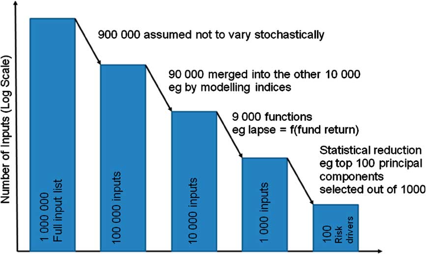
It is perhaps useful to consider the selection of risk factors via a hypothetical example. One can imagine that the number of inputs that affect the balance sheet of a firm that can be modelled stochastically is in excess of a million (this could easily be true assuming you count separately each number in the input mortality tables, have a number of different business units and products, etc.), but that ultimately an internal model is constrained to use as few as 100 risk drivers (Chart 4).

Chart 4 Simple illustration of how the number of risk factors compounds
The processes from reducing the 1,000,000 to 100 could include:
• ignoring some drivers because they are deemed to be deterministic or “insignificant”;
• using some as proxies for others;
• making some risk factors a function of others;
• more quantitative approaches such as principal component analysis (PCA) (Chart 5).
Chart 5 Simple illustration of how risk factors to include in the capital model might be obtained

In addition to the selection methods alluded to above, there are many algorithmic approaches used to identify those variables that minimise the measurement of predictive error subject to constraints of the size of any subset studied. Algorithmic approaches typically carry out a feature selection by including extra variables one at a time when carrying out the process in a forward manner, or exclude variables one at a time when carrying out the process in a backward manner. Of course, one needs to be careful when interpreting p-values associated with adding or removing variables problematic with this approach, as each is conditional on prior inclusion or exclusion of variables. In addition, any R 2 value may be overestimated, if based on the number of degrees of freedom from using the fitted variables, rather than the number of degrees of freedom used up in the entire model fitting process.
3.2. Dimension Reduction
This section focuses on the final step in the diagram overleaf, which considers the reduction in a large number of stochastic variables to a smaller number of important or “principal” factors.
3.2.1. PCA
This is a statistical method that transforms data from a high dimension space into a space of reduced dimension. A subset of new features from the original features in the data is performed by means of functional mapping techniques that aim to keep as many features as possible of the original data set. PCA is one of the most commonly used feature extraction techniques.
PCA uses an orthogonal transformation to convert a set of observations of correlated variables into a set of orthogonal principal components. The number of principal components is less than or equal to the number of original variables. PCA is a heavily researched statistical technique and already has a lot of applications in finance. For detailed examples in the context of interest rate modelling, refer to Lazzari & Wong (Reference Lazzari and Wong2012).
Deciding which factors to retain in the model can be based on the following techniques:
a) The eigenvalue-one criterion: also known as the Kaiser criterion, components are retained that have an eigenvalue greater than or equal to 1, that is, the retained variable is accounting for a greater amount of the variance than that contributed by one variable.
b) Proportion of variance retained: retain a component if it accounts for a threshold percentage, for example, 5% or 10% of the total variance, where the proportion of variance retained is given by: eigenvalue for component of interest/Σ (eigenvalues of correlation matrix).
Non-linear dimension reduction techniques extend these ideas based on non-linear mappings. Again, the principle is the same, maximising the variance in the resulting data set relative to the variance in the original data set.
The single biggest criticism of PCA in finance is that it is a pure statistical technique and ignores any economic or real-world causalities. Thus, it needs to be used and interpreted very carefully to avoid data mining and spurious accuracy. For example, you do not want to inadvertently have one of the important risk factors of your model be the size of Brazilian coffee beans, simply because the time series was included in the set of regression variables and provided an almost perfect fit. Although this is an extreme example that is obviously nonsensical, the lesson is that pure statistical models would be blind to this. More importantly, there may be many other significantly more subtle areas where the models are inadvertently subject to data mining.
Another criticism is that pure PCA factors are simply a linear combination of many variables and would lack intuition, as well as being subject to changes over time that are hard to explain.
The main mitigant of inadvertent data mining is for there to be expert human intervention at key stages of the process, choice of regression inputs through to sense checking and validation of the output results. Some of these are discussed in the next section.
3.2.2. Direct Choice of Principal Factors
This is another technique that is also commonly used alongside the PCA approach. This method directly chooses what are thought to be the principal factors so as to arrive directly at a fitted model, without recourse to any dimension reduction technique being applied. As such, this approach relies hugely on the skill or otherwise of the modeller in picking the appropriate modelling random variables that best satisfy the “eigenvalue-one” criterion and/or the “maximising the proportion of variance retained” criterion discussed above.
Although this approach could be very efficient in the presence of a skilled modeller, it suffers from the same drawbacks as per other aspects of judgement. In addition, the subjective element reduces the transparency of the choice components if not properly documented.
3.2.3. Hybrid Methods
In practice, neither a purely statistical nor a purely judgemental method is used. The method often adopted is a combination of the direct choice of principal factors and statistical techniques. Although this may often be done implicitly, it may be useful to be aware of the judgement and statistical steps explicitly, so as to avoid the worst pitfalls of each method.
Also important is the need to be aware of areas where selection of risk factors can cause potential problems. Some possible pitfalls are:
a) The model may have been subject to too wide a range of explanatory variables, resulting in inadvertent data mining.
b) The most important factors may have been wrongly selected or not selected at all, giving spurious and misleading results.
c) Presence of correlated variables results in a risk of a more intuitive/direct explanatory variable killed for another less intuitive/useful variable.
d) If the factors selected mechanically have not been validated, there is a risk that some inappropriate factors have been inadvertently included.
e) The weighting of the different factors may change over time. Factors that may have had an influence in the past may dissipate over time, whereas the opposite may be true of other factors.
f) Exogenous factors, for example, a change in external regulatory or commercial environment may change the nature of the problem and one needs to remember to revisit the choice of random variables in the selection process (i.e. there may be some “emerging” risk factors).
3.3. Grossing-Up Techniques
Acknowledging that there are practical limitations to the number of risks that can be modelled, some effort needs to be made to “gross up” the capital (i.e. make a capital allowance for the risks that have not been explicitly modelled). Thus, having gone through the selection (and perhaps) reduction of risk factors to come up with a capital model, one should take care not to forget these steps when estimating the total capital.
For example, as a very crude calculation, you might think that reducing 1,000,000 to 100 risk drivers, the resulting SCR should be grossed up by a multiple of 10,000. Most of us would probably say that is too big as there has been some effort to pick the most important of the 1,000,000 within the 100, but it is still likely that some important risks get squeezed out. Moreover, this only considers the risk factors that have been identified but not modelled (and does not delve into the unknown).
In principle, there is a strong relationship between grossing-up methodology and willingness to update models/incorporate new risks. If your initial SCR contains an explicit gross-up factor, then it is reasonable to release some of that factor as modelling becomes more detailed and comprehensive. If there is no grossing up, then every new risk you model causes a higher SCR, and therefore one might struggle to find acceptance within the business.
In addition to the basic grossing-up techniques for risk factors that may have been identified but not modelled described above, the following grossing-up techniques following dimension reduction are suggested below. Where the commonly used PCA approach has been used, it should be possible to apply both grossing-up techniques discussed below.
3.3.1. R 2 Adjustment
Following dimension reduction, a computation of the R 2 value can be compared between the original data set and the data set following dimension reduction. As noted above, the R 2 value in the dimensionally reduced data set will be an overestimate based on number of degrees of freedom used in the fitted variables, rather than the degrees of freedom used in the fitting process. A possible approximate grossing-up factor may be undertaken as follows:
 $$\frac{{{\rm{(Adjusted) }} \,{{R}^{\rm{2}}} \ {\rm{value}} \ {\rm{in}} \ {\rm{dimension - reduced}} \ {\rm{data}} \ {\rm{set}}}}{{{{R}^{\rm{2}}} \ {\rm{value}} \ {\rm{in}} \ {\rm{original}} \ {\rm{data}} \ {\rm{set}}}}$$
This only allows for the PCA element. A suitable margin for prudence should also be incorporated, to allow for any potential missed features in both the original data set and the dimensionally reduced data set that could affect results significantly in the future.
3.3.2. R Eigenvalue Grossing-up Factor
Compute the eigenvalue correlation matrix for both the components in the dimensionally reduced model and the original model. The grossing-up factor for the model then becomes:
 $$\frac{{\rSigma ({\rm{eigenvalues}} \ {\rm{of}} \ {\rm{correlation}} \ {\rm{matrix}} \ {\rm{of}} \ {\rm{original}} \ {\rm{model}})}}{{\rSigma {\rm{(eigenvalues}} \ {\rm{of}} \ {\rm{correlation}} \ {\rm{matrix}} \ {\rm{of}} \ {\rm{dimensionally}} \ {\rm{reduced}} \ {\rm{model)}}}}$$
Again a suitable prudence margin should be allowed for risk selection errors in the original model.
3.4. Stress and Scenario Testing
A possible method of estimating the impact of risks not modelled stochastically is to carry out a series of “sensitivity tests” to the model with changes in that deterministic variable. In addition, scenario testing is also useful, both as an addition to the aggregation methods applied and as an explanatory aid to senior management.
It should be noted that scenario and sensitivity testing could quite easily span a number of sections in this document as it is quite a broad method and can be used for a number of purposes. In addition to modelling non-stochastic risks and addressing some aspects of uncertainty on models and parameters, some specific examples of reasons why sensitivity testing is required are listed below.
• Not enough data for calibration of model – model uncertainty. An example of these is in the aggregation of capital owing to lack of data, there may be uncertainty as to the copula to use. For example, use of a Gaussian versus Student T copula. The impact of using an alternative copula can be tested;
• Not enough data for calibration of the parameters of a model – parameter uncertainty. An example of this is assessing the impact using a different loss, given default in deriving the capital for credit risk;
• Changes in conditions – the past may not be a good guide to what may happen in the future such as changes in interest rate regimes;
• Assessing the importance of assumptions made – the assumptions that have the most impact on the results can be determined by changing each assumption by the same proportion;
• Regulatory requirements such as “What if scenarios”, “reverse stress testing”, etc.
• Management information – an example of this is to assess the impact of different volumes of new business or different business mix on the capital strength of a firm in the next 3 years.
• Assessing the impact of different data sources used in the calibration of a model. For a lot of risks, there are alternative data sources. For equities, S&P500 or FTSE 100 or FTSE All Share indices can be used to calibrate the risk. A sensitivity test can be undertaken in which the stresses derived from using different data sources are assessed.
• Assess the impact of prior beliefs. Most actuarial tasks involve a number of prior beliefs. Examples of prior beliefs in actuarial tasks include the distribution that the aggregate capital of a fund or company is assumed to follow. Sensitivity testing allows the impact of these assumptions to be assessed.
A detailed example of scenario and stress testing related to aggregation methodology is provided in the next section.
3.4.1. Stress and Scenario Testing: an Example
In this section, the results of a case study to assess the impact of the use of different copulas models are investigated.
This case study assesses the impact of prior beliefs, especially when there are not sufficient data to be conclusive about the assumption being made. It involves assessing the impact on aggregate capital when different types of copulas are used to aggregate individual capital requirements.
The copulas used in these case studies are the copulas that lend themselves easily to aggregate more than two risks. As such copulas such as Gumbel, Clayton and Frank are not considered.Footnote 4
In the first case, the marginal distributions are all assumed to be normally distributed as shown in Table 2. Another case study is presented later in which different marginal distributions are assumed. We assume that we have the following risks with the distributions as specified in Table 2.
Table 2 Marginal risk factor distribution

The risks are assumed to be correlated as per Table 3.
Table 3 Correlation between risk factors

The aggregate capitals based on the following copulas are assessed:
a. correlation matrix;
b. normal;
c. Student T with different degrees of freedom.
The results of using different copulas are set out in Table 4.
Table 4 Capital required by type of copula

It is worth noting that when the marginals are all elliptically distributed (e.g. normal, Student T) the results of a normal copula and correlation matrix should be very similar, with any difference arising because of an inadequate number of simulations used in the Monte Carlo simulation.
Another sensitivity test was undertaken in which the marginal distributions were not all normally distributed. The distributions used are set out in Table 5. The parameters and the distributions were selected such that the capital of the marginal distributions was the same as that of the normal distributions above.
Table 5 Sensitivity - the effect of some risk factors not being normally distributed

1Note that the mean and standard deviation do not refer to lognormal distribution, but to its logarithm.
The results of this sensitivity are shown in Table 6.
Table 6 Sensitivity - capital required when some risk drivers are not normally distributed

The sensitivity testing as described in the case study above can be used to assess the range of values that the aggregate capital can assume, given the uncertainty about the appropriate dependency approach to use. It is important to note that this covers just one aspect of sensitivity testing, and that this would ideally need to be repeated for all of the key decisions in the capital calculation framework.
3.5. Key Points
The selection of what risk factors to model stochastically is a crucial choice within capital models, and deserves a great deal of attention. We illustrate this by an example where a very large number of potentially stochastic inputs are compressed to merely 100 risk drivers. We discuss the possible range of factor-reduction methods at the final stages of the selection and highlight some potential pitfalls in the process.
We also explain the importance of “grossing up” for all the risk factors that are not modelled stochastically, by considering the link between grossing-up methodology and willingness to update models/incorporate new risks.
Finally, we discuss the idea of scenario and stress testing, together with a worked example on capital aggregation.
4. Model and Parameter Error
4.1. Allowing for Model and Parameter Risk
With the “appropriate” model and “accurate” assumptions, we can justify statements such as “with €100 m of available capital, there is a 99.5% probability of sufficiency one year from now”.
However, given that a model is only intended to be a representation of reality, it is unlikely any model will be ever fully correct, or the assumptions fully accurate. This section considers how such a statement may be modified if a firm has concerns about the correctness of models or accuracy of parameter estimates. There might be several models that adequately explain the data. Even when one model is a better fit than another, we may not be able to reject the worse fitting model as a possible explanation of the data. There is a difference, however, between picking one model as the most credible explanation and picking one model as the only credible explanation. We should not discount the possibility that some initially less plausible model could subsequently turn out to be the most appropriate.
Model error is one of many risks to which financial firms are exposed. We might hope to quantify model error in much the same way as other risks, by examining the potential losses arising from model mis-specification. These might then be incorporated into a risk aggregation process, making appropriate assumptions about the correlation between model risk and other risks.
In this section, we argue that model risk is of an essentially different nature to other modelled risks. To describe interest rate risk, we take as given a model of how interest rates might move, test the model against past data and use this model to explore the likelihood of possible adverse shocks. A probability approach is ideal for such an analysis. The probability framework is less equipped to cope with ambiguity in models. For example, we may struggle to find an empirical basis to express the likelihood of alternative models being correct.
Several different models might account for the historic data, but they might have different implied capital requirements. Percentile-based capital definitions no longer produce a unique number, but rather a scatter of numbers depending on which model is deemed to be correct. If we want the answer to be a single number, then we have to change the question.
We then give concrete examples of model and parameter risk. We consider possible ways of clarifying the 99.5%-ile question in the context of model ambiguity and explore the impact on model output.
It is helpful to consider model ambiguity in three stages:
• Models and parameters are known to be correct. This is the (hypothetical) base case to which we compare other cases.
• Location scale uncertainty (section 4.1.1): past and future observations are samples from a given distribution family, but the model parameters are uncertain. Specifically, we consider situations where candidate distributions are related to each other by shifting or scaling.
• Model and location scale uncertainty (section 4.1.2): both the applicable model and the parameters are uncertain. For example, there may be some dependence between observations and the observations may be drawn from one of a family of fatter-tailed distributions. In each case, limited data are available to test the model or fit the parameters.
4.1.1. Parameter Uncertainty in Location Scale Families
We consider an example where the underlying model is of a known shape, but where the location and scale of the distribution are subject to uncertainty. This is usually the case in practice.
We then consider three possible definitions of a percentile where parameters are uncertain (Table 7).
Table 7 Possible percentile definitions when there is parameter uncertainty

It is not always clear in practice, even for statutory purposes such as computing the solvency capital requirement, which, if any, of these definitions applies.
4.1.2. Comparison of Statistical Definitions to Actuarial Best Estimates
We contrast probability definitions with actuarial concepts of best estimates, as discussed, for example by Jones et al. (Reference Jones, Copeman, Gibson, Line, Lowe, Martin, Matthews and Powell2006):
“best estimates … contain no allowance or margin for prudence or optimism”.
“… they [best estimates] are not deliberately biased upwards or downwards”.
“The estimates given in the report are central estimates in the sense that they represent our best estimate of the liability for outstanding claims, with no deliberate bias towards either over or under-statement”.
The actuarial best estimate definitions refer to a lack of deliberate bias. This suggests that provided the actuary did not intend to introduce bias, a “best estimate” results. If there turns out to be a bias in a statistical sense, this does not disqualify an actuarial best estimate provided the bias is unintentional. This highlights the difference between actuarial best estimates defined in terms of intention and statistically unbiased estimates defined in a mechanical way.
Our statistical definitions refer to probabilities that can in principle be tested in controlled simulation experiments, and indeed we will conduct such experiments in the example that follows. As defined above, any best estimate is a point estimate. However, there is an interval of plausible outcomes around this estimate. There are different statistical definitions for such an interval. The experiment that follows considers two of these intervals (described in section 4.1.1):
• substitution: β-quantile;
• confidence interval with probability γ containing the β-quantile;
• prediction interval containing the unseen observation with probability β.
What the experiment shows is that the properties of a probability distribution do not necessarily determine a unique construction for an interval. There might be (and indeed, there are) several ways to construct intervals satisfying the definitions.
4.1.3. Five Example Distributions
We now show some example calculations of these intervals based on five distribution families. In each case, we define a standard version of a random variable X; the other distributions in the family are the distributions of sX + m where m can take any value and s > 0.
Our five distributions include fatter- and thinner-tailed examples, and include asymmetric distributions (Table 8).
Table 8 The five example distributions and their properties

Our families consistent of cumulative distribution functions
 $$$F\left( {\frac{{x\,{\rm{ - }}\,m}}{s}} \right)$$$
and density
$$$F\left( {\frac{{x\,{\rm{ - }}\,m}}{s}} \right)$$$
and density
 $$$\frac{1}{s}f\left( {\frac{{x\,{\rm{ - }}\,m}}{s}} \right)$$$
, where F and f are taken from a (known) row of Table 8.
$$$\frac{1}{s}f\left( {\frac{{x\,{\rm{ - }}\,m}}{s}} \right)$$$
, where F and f are taken from a (known) row of Table 8.
Chart 6 shows these probability density functions. We have chosen values of m and s for each family to make the distributions as close as possible to each other.
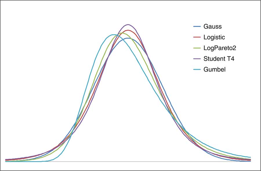
Chart 6 Probability density functions of the five example distributions
4.1.4. Methods of Estimating Parameters
We consider four ways of estimating model parameters given a random sample of historic data (Table 9).
Table 9 Four methods of estimating model parameters

4.1.5. Interval Calculation
We now provide algorithms for calculating the different types of intervals (Table 10).
Table 10 Algorithm for calculating the different types of interval

When talking about probabilities, care needs to be taken with respect of the set over which averages are calculated. The frequentist methods (method of moments, probability weighted moments, maximum likelihood) measure probabilities over alternative data sets. The Bayesian statements average over possible alternative parameter sets but not over any data sets, besides the one that actually emerged. A 99.5% interval under a frequentist approach is not the same as a 99.5% Bayesian interval.
We use Monte Carlo methods to calculate confidence and prediction intervals. We show these in the case of 20 data points, using the method of moments, based on the 99.5%-ile. These measures differ only because the data are limited; as the data increase these are all consistent estimators of the “true” percentile. None of these is *the* right answer; the different numbers simply answer different questions (Chart 7).
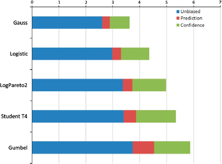
Chart 7 Illustration of various interval definitions for the five example distributions
The interval size (expressed as a number of sample standard deviations) varies from one distribution to another. Note that, although the T4 distribution has the fattest tails in an asymptotic sense (it has a power law tail, whereas the others are exponential), the Gumbel produces the largest confidence intervals. This is because the asymptotic point at which the T4 distribution becomes fatter lies way beyond the 99.5%-ile in which we are interested.
We also consider how the intervals vary by the number of observations. The prediction intervals are shown below. We can see that the prediction interval requires a smaller number of standard deviations as the sample size increases, because a better supply of data reduces the errors in parameter estimates (Chart 8).
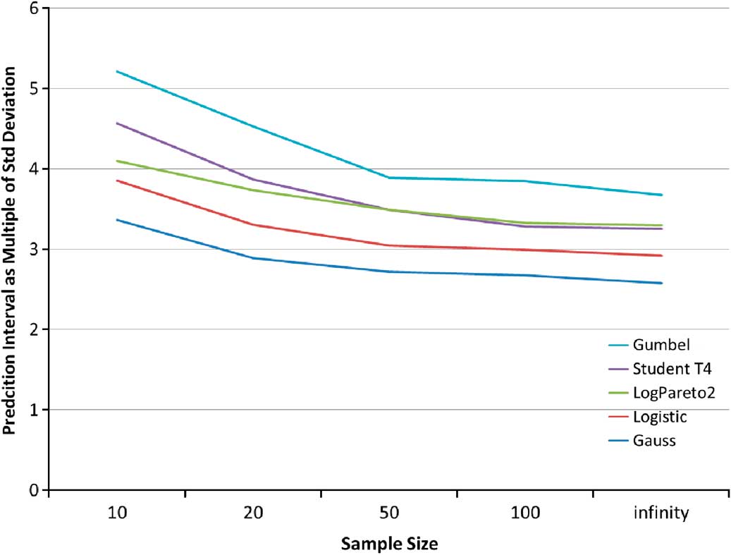
Chart 8 Prediction Interval variation by sample size for the five example distribution
4.2. More on Model Risk
We have described ways of calculating 99.5%-iles in the presence of parameter risk, at least in the case of location scale probability distribution families.
Uncertainty about shape parameters or about underlying models is more difficult to address. The difficulty is constructing an interval that covers 99.5% of future outcomes, uniformly across a broad family of models. In general, the best we can hope is an inequality, so that at least 99.5% is covered.
We set out two examples of the impact of using different models to estimate variables of interests. These show that the choice of the models has a very material impact of the estimate of the variable of interest. We then set out some techniques that can be used to assess the impact of model errors. The techniques described later are by no means an exhaustive list, but a list of the techniques commonly used in practice.
4.2.1. Example of Model Risk
A recent paper by Richards, Currie and Ritchie compares seven different models of longevity. They compare the value of a life annuity with a 70-year-old man, limited to 35 years and discounted at 3%. The paper constructs a probability distribution forecast for this annuity in 1 year's time using different models of mortality improvements. We reproduce table 5 from that paper below (Table 11).
Table 11 Comparison of average annuity value and percentile estimate by different longevity models

.
Please refer to the paper by Richards et al. (2014) for more details about the mortality models. We might hope for a degree of consensus between the different modelling approaches, but these figures show the opposite. Indeed, a future annuity value of 12.5 lies below the mean for two of the models, but above the 99.5%-ile for two other models (http://www.actuaries.org.uk/sites/all/files/documents/pdf/value-risk-framework-longevity-risk-printversionupdated20121109.pdf).
4.2.2. Another Example: Gauss and Gumbel Distributions
Let us return to the set of five probability distributions described in section 4.1.3. The distribution functions are sufficiently close that the curves are difficult to distinguish by eye. However, we can separate them by subtracting one of the cumulative distribution functions, for example, the logistic. Chart 9 shows the CDF for each distribution minus the logistic CDF.
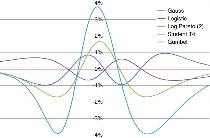
Chart 9 Illustrating the difference in the CDF of the five example distributions, measured relative to the logistic
Although these distributions have different shapes, the distribution functions differ nowhere by more than 4%. This suggests that it will be difficult to separate the distributions using statistical tests based on small sample sizes.
Goodness-of-fit tests such as Kolmogorov–Smirnov and Anderson–Darling have low power when data are scarce. Table 12 shows the power of KS and AD tests with 20 data points. The chance of rejecting an incorrect model is often only marginally better than the chance of rejecting the correct model, and in a few cases the correct model is more likely rejected than an incorrect one.
Table 12 Probability of Rejecting a Model Fitted Using the Method of Moments Tested Using a Kolmogorov–Smirnov (or Anderson–Darling) Statistic Based on 95% Confidence and 20 Observations

Even with samples of 200 or more, it is common not to reject any of our five models. This implies that model risk remains relevant for applications including scenario generators, longevity forecasts or estimates of reserve variability in general insurance.
4.3. Techniques to Assess Model Errors
The examples described above shows that there are a range of models that can be used to undertake a task. This motivates a quest to understand any error introduced by model choice.
Model risk remains relevant for virtually all aspects of actuarial modelling, from longevity forecasting to capital aggregation. Are we then at risk of channelling too much energy and expense into the “holy grail” route of modelling, justifying each parameter and component of a single model? Does our governance process consider model risk, or does board approval for one model implicitly entail rejection for all others?
Given the inevitable uncertainty in which model is correct, how can we make any progress at all? There are several possible ways to proceed:
• Pick a standard distribution, for example, the Gaussian distribution, on the basis that it is not rejected. The statistical mistake here is to confuse “not rejected” with “accepted”.
• Taking the prudent approach – the highest 99.5%-ile from all the models.
• Build a “hyper-model”, which simulates data from a mixture of the available models, although expert judgement is still needed to assess prior weights. Ian Cook (Reference Cook2011) has described this approach in more details on the context of catastrophe models.
Industry collaboration on validation standards may lead to generally accepted practices. For example, over a period of time practice may converge on a requirement to demonstrate at least 99.5% confidence if the data happen to come from a Gaussian or logistic distribution, but not for Student T or Gumbel distributions. This may not always be a good thing, particularly if it leads to a false sense of security.
A commonly used mitigant against model and parameter error already in use within the industry is to carry out scenario- and stress-testing approaches. These were described in section 3.4. A more statistical technique that may prove useful is the concept of robust statistics and ambiguity sets described below.
4.3.1. Robust Statistics and Ambiguity Sets
Robust statistics is the study of techniques that can be justified across a range of possible models rather than a single model. It can be used to help derive prediction intervals that are robust to the choice of distribution.
Suppose using the method of moments we wanted to construct a prediction interval of the form
 $$$\left( {{\rm{ - }}\infty, \hat{\mu }\, + \,y\hat{\sigma }} \right)$$$
valid across a class of distributions (this set is known as the ambiguity set). We cannot achieve exact α-coverage for all distributions. We can, however, achieve at least α-coverage for a class of distributions simply by taking the largest y across that class. For example, we might specify that the methodology should cover at least a proportion α of observations X n + 1 for an ambiguity class, including Gaussian and logistic distributions. In this case, our chart in section 4.1.4 shows that the logistic distribution produces the highest y, and therefore the prediction interval is defined based on the logistic distribution, knowing this is conservative for other distributions in the specification of the ambiguity class.
$$$\left( {{\rm{ - }}\infty, \hat{\mu }\, + \,y\hat{\sigma }} \right)$$$
valid across a class of distributions (this set is known as the ambiguity set). We cannot achieve exact α-coverage for all distributions. We can, however, achieve at least α-coverage for a class of distributions simply by taking the largest y across that class. For example, we might specify that the methodology should cover at least a proportion α of observations X n + 1 for an ambiguity class, including Gaussian and logistic distributions. In this case, our chart in section 4.1.4 shows that the logistic distribution produces the highest y, and therefore the prediction interval is defined based on the logistic distribution, knowing this is conservative for other distributions in the specification of the ambiguity class.
Robustness for a given ambiguity class says nothing about models outside the class. We might construct prediction intervals robust across uniform, normal and logistic distributions, but these intervals would not be valid for Gumbel distributions. They would also not be valid if other assumptions are violated – if the observations are not independent or are drawn from more than one distribution.
The size of the ambiguity set is a key determinant of prediction interval size. A bigger ambiguity set means a harsher test of coverage and larger prediction intervals. It also means more wastage, in the sense that if the true distribution is one of the more benign from the ambiguity set, then the prediction interval will contain a higher than intended proportion of future observations.
Nassim Taleb (2007) has popularised the notion of “Black Swan” events, that is, unpredictable events that arise with no prior warning (and by definition unpredictable with models that existed before the event happening). Models popular in the mid-2000s, many based on Gaussian distributions, were criticised for producing too few Black Swan events and therefore understating risks. Black Swan events also highlight the classic philosophical “problem of induction” that inference from past events can only work to the extent that the same model applies in the past as in the future. We could define a “Black Swan” model as one where one set of formulas applied until yesterday, and tomorrow another unrelated set of formulas takes over. There can be no robust statistical procedure that works for such models as the past data are of no value for future inference. It may potentially be the case that the world has fundamentally and unrecognisably changed, but one also needs to be extremely careful that less likely models are not rejected early on in the decision-making process in favour of the most plausible model without allowing for model risk. One conclusion is that any claims of robustness with respect to a statistical procedure should include a careful description of the ambiguity set against which the procedure is robust.
4.4. Key Points
This section focused on model and parameter error and considers in details two cases, where observations are from a given distribution, but there is uncertainty about the parameters (parameter error) or where we are uncertain about the actual model itself (model error).
It also highlighted the important case that when we have model or parameter uncertainty, the capital estimation problem itself is not unambiguous, going on to discuss three possible definitions of a percentile where parameters are uncertain. We also provided an extended example, based on different methods of estimating parameters and based on different possible distributions.
Finally, we also discussed different techniques to assess model errors, and introduced the idea of robust statistics and ambiguity sets, which look at techniques that apply over a range of candidate models, rather than a single model that is considered to be most plausible, finishing with a caution to properly allow for model risk before labelling too many events as “Black Swans”.
5. Errors Introduced by Calculation Approximations
So far, we have looked at errors in the process of trying to build the best model, while acknowledging that any model is at best a representation of reality. However, in practice, the models are not always run to their full capacity in terms of granularity or number of simulations.
In particular, over the last few years, there has been a rise in so-called proxy (or “lite”) models, which purport to have a good approximation of the more established “heavy” models. These approximations are usefully introduced in the interest of faster run times and quicker reporting, and may include the approximation of asset and liabilities by simpler polynomials and/or running a limited number of simulations.
Section 5.1 looks at the types of errors that can arise from the proxy model approximations, whereas section 5.2 tackles Monte Carlo sampling error. In addition, some simplified insurance assets and liabilities are described for the purpose of testing proxy models in capital aggregation calculations, and some lessons presented.
5.1. Proxy Models
Insurers’ assets and liabilities are complicated functions of millions of inputs whose future values are uncertain. The inputs include market prices of assets and financial instruments, incidence of events giving rise to insured losses, and vast tables of experienced and projected actuarial decrements such as mortality or attrition. Insurers use “heavy models” to compute the value of assets and liabilities as functions of the long list of inputs.
In theory, insurers are supposed to perform full stochastic projection to demonstrate there is a relatively high probability that, in future, assets will exceed the value of liabilities. This means:
- simulate millions of joint scenarios;
- in each scenario, the asset and liability functions are evaluated using a heavy model fed from the millions of jointly simulated input variables.
In cases where a market-consistent valuation of a complex, path-dependent option is required for each real-world simulation, the well-known “nested stochastic” situation arises. In this structure, a set of market-consistent simulations is required for each “real-world” scenario.
Despite advances in computer calculation speed and storage capacity over the last few decades, a full stochastic projection remains beyond the reach of most insurers. Instead, there is a widespread use of simplified “proxy” models. These are simple functions of a small number of variables intended to approximate the heavy model output, usually expressed as a sum of terms whose coefficients are estimated by fitting to heavy models. While running the heavy model millions of times is costly, this number of proxy model evaluations is easily feasible.
The functions that make up the proxy models are referred to as basis functions.
5.1.1. Spanning Error
The method of proxy functions assumes that the true assets and liability functions are of the chosen form, or can be approximated sufficiently accurately by functions of that form. This assumption could fail severely, for example, if:
• Assets and liabilities depend on inputs that have been excluded in the selection of risk factors to model, through the dimension reduction process discussed previously. Thus, the behaviour of assets and liabilities are not sufficiently explained by the retained risk factor inputs.
• The true function has a “cliff-edge” (i.e. a discontinuity), whereas all the basis functions are continuous. More subtly, the true function could have a kink (i.e. point where it is not differentiable), whereas the basis functions are assumed to be continuously differentiable.
• The assets and liabilities have “sink holes”, that is, regions of parameter values where assets collapse or liabilities explode, whereas none of the basis functions exhibit this behaviour.
• The asymptotic behaviour of the liabilities is simply different from the functions chosen. This is not an uncommon occurrence, because polynomials (apart from constants) tend to ±∞, whereas guaranteed liabilities would tend to 0 when they are out of the money and ∞ when in the money.
These are all examples of “spanning failure”, where the true assets and liabilities are not in the linear span of a proposed set of basis functions. The “spanning error” is any mis-statement in the required capital that arises from spanning failure. We set out some approaches that can be used to validate proxy models through case studies in the sections that follow.
5.1.2. Selected Test Models
We construct test valuation formulas based on three risky asset classes: government and corporate bonds, equities and a risk-free cash asset. We consider three lines of business: regular premium term assurance, a life annuity and a single premium-guaranteed equity bond. We use simplified policy models so that exact valuation is possible with closed formulas, based on nine risk drivers: risk free rate, equity price, equity volatility, corporate bond spread, liquidity premium, mortality (term and annuity) and lapses (term and guaranteed equity).
This is a simplified set of risk drivers for ease of calculation. We use a single discount rate for risk-free cash flows of all maturities. The equity volatility is required for valuing the guarantee according to option pricing theory. We assume that annuities cash flow will be discounted at a discount rate that includes a return premium for holding illiquid assets. This is assumed to be assessed with respect to the observed yield spread on a class of illiquid asset subject to credit rating criteria.
Our firm also holds corporate bonds. The change in value of these bonds is driven by changes in bond spreads, but in this case we need to follow the fate of a fixed portfolio of bonds rather than tracking typical spreads for a particular grade. This distinction implies that a portfolio of bonds cannot perfectly hedge the liquidity premium assessed in relation to a particular grade.
The formulae for the assets and liabilities described in the table overleaf are detailed in Appendix B.
5.1.3. Curve Fitting Methodology – Annuity Case Study
To illustrate the issues involved, we start by approximating the annuity examples, using polynomials in the discount rate (which we denote by r) and in the maximum lifetime (denoted by t). There are several different ways to build up polynomials of increasing order. We have considered the following four ways (Table 13).
Table 13 Possible ways to construct polynomials for curve fitting

5.1.3.1. Least Squares Results
We calculated least squares estimates using a 101-step grid for each of the two risk drivers, that is, a 101 × 101 grid covering max lifetime between 0 and 20 years combined with discount rates between 0% and 25%. The Chart 10 below shows the minimised root mean square error (RMSE) as a function of parameter count (maximum 36) for each of our fit families.
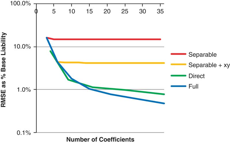
Chart 10 Root mean square error against parameter count by type of fitting polynomial
Chart 10 shows how the fit improves as the number of coefficients increases. The results show that the separable formula, with or without the xy terms, quickly gets stuck. Adding higher order polynomials in just one variable has a negligible impact on the RMSE. Instead, it is necessary to add sufficiently rich joint powers alongside the univariate powers to achieve convergence.
The chief advantages of the least squares method include:
• It is known to have a unique solution provided the number of sample points exceeds the number of fitted coefficients.
• Finding that unique involves the relatively straightforward solution of simultaneous linear equations. In addition to being readily soluble, it is also easy to demonstrate that a proposed solution satisfies the relevant equations and thus verify that the solution is optimal from a least square perspective.
• Beyond our particular example, where the liability is defined as the average of Monte Carlo simulations, there may be computational efficiencies by the use of least squares Monte Carlo techniques.
The chief limitation of least squares techniques is the difficulty of converting a RMSE into a bound in the accuracy of an estimated percentile. The problem is that the RMSE is an average of the errors; the error in a percentile estimate may be much larger because not all points have an equal impact on the percentile. Large percentile errors arise if the estimate is sensitive to the fit-for-risk driver values where the fitted proxy polynomial diverges most from the true function.
5.1.3.2. Regression Diagnostics
Statistical regression packages usually provide additional output, including R 2 statistics, parameter significance tests, confidence intervals and information criteria such as those of Akaike. We might hope these could provide a scientific basis for including or excluding terms in a polynomial. The derivation of these tools relies on various assumptions listed below (Table 14).
Table 14 Assumptions implicit in regression diagnostic tools

The standard statistical assumptions clearly do not apply in our example where the fitting is not even random and the underlying annuity function is not a polynomial. Such statistical tools overstate the effective number of observations by assuming that each new observation contains an independent model observation, whereas in our curve fit new observations are still from the same deterministic curve. The statistically derived intervals are spectacularly too narrow compared with the true error.
5.1.3.3. Minimax Calculations
We have described curve fitting by regression and the difficulty of translating a RMSE into an error in percentile estimates.
The situation is more straightforward if we consider the maximum error. If we know that the maximum error is bounded, for example, by 1% of the liability value (for all risk-driver values), then we know that our percentile estimates are also accurate to within 1% of the liability value.
In our regression examples, the maximum error is between five and ten times the RMSE, with the multiples generally increasing for models with more parameters. Note that any attempt to construct error bounds on the RMSE using probabilistic logic is doomed to failure, as in our cases the residuals are not generated from any probability distribution.
Performing a least squares fit does not minimise the maximum error. Minimising the maximum error requires a minimax fit, typically giving a different polynomial than the least squares. The minimax fit will by construction have a lower maximum error than the least squares fit, but a large RMSE. The reduction in maximum error is not spectacular; in most of our examples, the reduction was <50% of the least squares maximum error, although the available reductions tend to increase with larger parameter counts. However, the minimax fits are much more difficult to implement numerically, frequently beset by multiple solutions.
Finally, we note that the stated RMSE is a function of the size of the region over which the fit is measured. Had we chosen a smaller region, the stated RMSE would typically reduce. However, it would be wrong to conclude that the corresponding capital numbers have become more accurate, as the smaller region would then exclude a larger proportion of the risk scenarios over which the capital requirement is calculated.
5.1.4. Curve Fitting Methodology: Combined Model
We now develop tools for fitting curves to the actuarial formulas in a combined model of all risks. This can help us to evaluate the extent to which observed RMSE for each asset and liability type may translate into errors in estimated percentiles.
We fit curves to a series of stress tests. The stress tests are constructed using median values for each risk driver, as well as high (α-quantile) and low (1−α-quantile) values. For example, if α = 0.995 then we would calibrate to the 0.5%-ile, median (50%-ile) and 99.5%-ile for each risk driver.
We look at all combinations of high, median and low for each risk driver. This implies that with nine risk drivers, we may have to examine 39 = 19,683 stress tests. Thankfully, this is an overestimate, as our example assets and liabilities depend individually on at most four risk drivers. The maximum number of stresses is then 34 = 81 risk drivers, in the case of the guaranteed equity bond. The minimum number of stresses is three, for the risk-free bond and the equity, which depend on only one risk driver.
Having constructed the stress tests, we then fit a polynomial. In each case, we use ordinary least squares to fit the formula. We consider three fits based on the polynomials considered in the annuity example:
• Linear fit: we estimate assets or liabilities as a constant term plus linear terms in each risk driver.
• Separable quadratic fit: we estimate assets or liabilities as a constant term, plus linear and squared terms in each risk driver. This formula is still separable, that is, basic own funds is a sum of functions, each of which depends only on one risk driver. There is no mechanism for the level of one risk driver to affect the sensitivity of net assets to another driver.
• Quadratic fit with cross terms: assets and liabilities are a constant term, plus linear and squared terms in each risk driver, and also products of risk drivers taken two at a time.
We can consider extending these fits to cubic and higher order polynomials. However, we are unable to investigate such fits in our simple example, at least in the one-dimensional cases (equities and government bonds), because we have chosen to evaluate only three fitting points that are insufficient to estimate polynomials of higher than quadratic order.
5.1.5. Risk Driver Distribution
For demonstration purposes we assume that risk drivers have shifted lognormal distributions. We construct these using formulas of the form:
 $${\rm{riskdriver}}\, = \,{\rm{median}}\, + b\,\frac{{{{e}^{cZ}} \ {\rm{ - }}\,1}}{c}$$
where b is a positive coefficient, whereas c is positive or negative. If c = 0 we replace the fraction
 $$$\frac{{{{e}^{cZ}} \ {\rm{ - }}\,1}}{c}$$$
by its limiting value Z. This is readily calibrated to quantiles. For example, suppose for some k, the Φ(−k) quantile is median −α and the Φ(k) quantile is median + β, we have to solve the equations:
$$$\frac{{{{e}^{cZ}} \ {\rm{ - }}\,1}}{c}$$$
by its limiting value Z. This is readily calibrated to quantiles. For example, suppose for some k, the Φ(−k) quantile is median −α and the Φ(k) quantile is median + β, we have to solve the equations:
 $$\matrix { b\frac{{{{e}^{{\rm{ - }}ck}} \ {\rm{ - }}\,1}}{c}\, = \,{\rm{ - }}\alpha \cr b\frac{{{{e}^{ck}} \ {\rm{ - }}\,1}}{c}\, = \,\beta $$
From this, it immediately follows that
 $$\matrix { {{e}^{{\rm{ - }}ck}} \, = \,\frac{{{{e}^{{\rm{ - }}ck}} \ {\rm{ - }}\,1}}{{1\,{\rm{ - }} \ {{e}^{ck}} }}\, = \,\frac{\alpha }{\beta } \cr c\, = \,\frac{1}{k}\ln \left( {\frac{\beta }{\alpha }} \right) \cr b\, = \,\frac{{c.\alpha \beta }}{{\beta \,{\rm{ - }}\,\alpha }} $$
There is a special limiting case when α = β, where c = 0 and b = α/k.
Within the firm's internal models, there is no general rule relating the opening (t = 0) risk drive values to their future distribution. However, for simplicity in the current curve fitting tests, we assume that the opening values are equal to the median.
5.1.6. Some Simulated Results
Chart 11 shows a scatter of the basic own funds (for the whole company) based on fitted polynomials compared with the “true” result based on the exact formula, for 1,000 simulations. In a capital calculation, we are interested principally in the bottom left-hand side, which corresponds to low values of own funds.
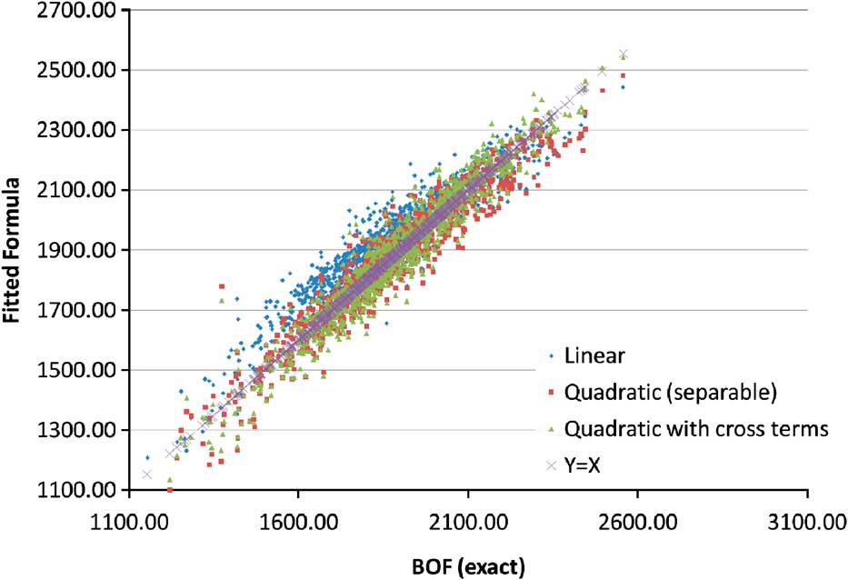
Chart 11 Actual BOF against BOF calculated by proxy formula by type of fitting polynomial
Overall, the quadratic with cross terms provides the best overall fit, which is not surprising as it has the largest parameter count. However, the deviations between the exact and fitted formula are substantial in places, and furthermore appear to show significant biases – for example, the linear regression overestimates BOF more often than it underestimates BOF.
This observation may at first seem odd; if the coefficients are estimated by regression, then surely the average residual should be 0. To resolve this paradox, we need to note that there are many different ways to calculate an average. The regression is an average over a small number of selected stress points, whereas our simulated BOF produces an average over a realistic distribution of risk drivers. We would not expect these averages to coincide. Indeed, biases in fits are commonly observed whenever the scenarios used for fitting a proxy model are not the same as those used for capital calculations.
Further investigations involving the elimination of negative reserves have revealed that discontinuities or kinks in the formulas need to be modelled as an additional layer. They cannot be well modelled using polynomial functions, even of very high order.
5.2. Monte Carlo Sampling Error
In this section, we consider two instances of Monte Carlo sampling error:
• That arising from the market-consistent valuation of options and guarantees (complex, path-dependent, options) by calculation of the discounted mean cash flows over a large number of randomly simulated scenarios.
• That arising in estimating the SCR, or more generally any quantile, by simulation.
In the particular case of market risk, the market-consistent simulations are likely to come from a risk-neutral economic scenario generator. The simulations for the SCR are likely to be “real-world” simulations.
In the ideal world assumed, the issue of Monte Carlo sampling is the only “error”. That is, we assume that the internal model has no missing risks and the modelling of the known risks is 100% accurate (the actual underlying risk driver can be modelled using the chosen risk drivers and the parameterisation of the risk drivers and loss functions is 100% accurate).
5.2.1. Market-Consistent Valuation and Monte Carlo Sampling
A market-consistent valuation of a complex, path-dependent liability will typically involve running a number of risk-neutral scenarios, from an appropriately calibrated economic scenario generator through a cashflow model. The mean of the guarantee and option cost, across all the simulations, is the market-consistent value of the guarantees. Furthermore, we can use the standard deviation of the individual scenario costs to calculate a confidence interval for the mean (i.e. the market-consistent cost of the guarantees and options in this instance) using the independent and identically distributed property and the central limit theorem. It is worth noting that estimation of the confidence interval as shown below applies under some strict conditions, such as the variable in question being normally distributed and the suitably large number of scenarios:
 $${\rm{95\%, }} \ {\rm{two}} \ {\rm{sided,}} \ {\rm{confidence}} \ {\rm{interval}} \ {\rm{for}} \ {\rm{mean}} \ {\rm{ = }}\,\hat{\mu }\, \pm \,{\rm{1}}{\rm{.96}}\frac{\sigma }{{\sqrt N }}$$
Various variance reduction techniques can be applied to make the valuation converge more rapidly – antithetic sampling, control variates, stratified sampling, importance sampling and low-discrepancy numbers (Sobol, Niederreiter, etc.). When using these techniques, the assumption of independent and identically distributed scenario outputs may not be valid.
Occasionally, situations arise, associated with sampling error, which can trap the unwary. For example, consider 1,000 observations from a lognormal distribution whose parameter (the standard deviation of the log) is β. Each observation is of the form exp(β.Z) for some Z ≅ N(0,1). When β is large (and hence the distribution is most skewed) the interval
 $$\left( {\hat{\mu } \ {\rm{ - }}\,1.96\frac{{\hat{\sigma }}}{{\sqrt N }},\;\hat{\mu } \ {\rm{ + }}\,1.96\frac{{\hat{\sigma }}}{{\sqrt N }}} \right)$$
is dominated by the term exp(β.Z max) where Z max is the largest observation. However, we know that the true mean is exp(β 2/2) and that for large β it is pretty certain that the true mean lies outside the confidence interval. In this case, it would be much better to recognise the data as lognormal and take logs of the data and estimate the parameters using analytical formula. The reason for this is that the above formula for determining confidence interval is based on the assumption that the variable of interest is normally distributed. Thus, when the distribution followed by the variable is highly skewed, then the above formula would not be applicable.
In cases such as this it seems useful to have some room to override the standard approach – the example described here is relevant to out-of-the-money guarantee costs.
5.2.2. Quantile Estimates and Monte Carlo Sampling
It is useful to start by considering the base case of an internal model using real-world simulations of risk drivers and loss functions. It is desirable to know the sampling error in the SCR estimate that is obtained from an ordered series of losses from a run of the internal model.
At a naïve and qualitative level, the degree of sampling error can be assessed by examining the distribution properties of the ranked internal model output. If the losses around the 99.5% simulation are “smoothly distributed”, tightly grouped and lie within the same range, then the sampling error will be small. Equivalently, we can look at the distribution of the 99.5%-ile simulation from a repeated sampling of the internal model with different random number sequences (but with all other parameters left unchanged). Obviously, we will need to recheck if these distribution properties apply for each recalibration of the model.
The estimation of quantiles can be considered at a more mathematical level. First, defining a notation for a quantile as Qα (b.X) where:
• α is a probability between 0 and 1;
• X is a random vector, which might represent profits from different business units or risk types;
• b is a vector of multipliers, reflecting a firm's exposure to each business or risk type.
The given data take the form of n observations of a random vector X, assumed to be a random sample from some distribution. For historic data, the assumption of a random sample may be open to challenge. However, in some applications, we are seeking to estimate percentiles from data that have been generated from Monte Carlo simulation; in that case, we can be more confident that the observations truly are independent samples from a common distribution.
The estimation of a quantile is often an intermediate step in a longer calculation. For example, a firm may wish to understand the sensitivity of a percentile to the selected risk exposures, which means calculating the sensitivities of the quantile Qα to the exposure vector b. There may be some form of optimisation involved, for example, finding multipliers to maximise expected profit subject to constraints on financial strength that might be expressed in terms of extreme quantiles.
In the simplest case, we can directly estimate the quantile from the empirical distribution function – here we refer to this approach of quantile estimation as direct percentile estimation.
5.2.2.1. Direct Percentile Estimation
To ease notation, we consider the scalar case. Suppose then we have n independent scalar observations X 1, X 2, .., Xn .
We can sort this into increasing order, denoting the sorted variables with subscripts in parentheses: X (1) ≤ X (2) ≤ … ≤ X ( n ).
The empirical cumulative distribution function is given by
 $$\hat{F}(k)\, = \,\frac{1}{N}\mathop{\sum}\limits_{i\, = \,1}^N {\chi \{ {{X}_i}\,\leq \,k\} } \, = \,\frac{1}{N}\mathop{\sum}\limits_{i\, = \,1}^N {\chi \{ {{X}_{(i)}}\,\leq \,k\} } $$
This is the average of a series of step functions and is easily seen to be an unbiased estimate of the true cumulative distribution function. The corresponding right continuous inverse is (for 0 ≤ α < 1):
 $${{\hat{F}}^{{\rm{ - }}1}} (\alpha )\, = \,X\left( {1\, + \,\left\lfloor {N\alpha } \right\rfloor } \right)$$
where X(i) denotes the i th sample value of X, in increasing order. This provides the most basic estimate of sample quantiles.
5.2.2.2. Direct Percentiles: Exact Distribution
We can construct the cumulative distribution function of the sorted observations X ( r ) in the important special case where the true distribution function F(x) is continuous.
The exact distribution of the r th observation is a transformation of the β distribution (this is readily proved by induction):
 $${\rm{Prob}}\left\{ {X(r)\,\leq \,x} \right\}\, = \,\frac{{\rGamma (n\, + \,1)}}{{\rGamma (r)\rGamma (n\,{\rm{ - }}\,r\, + \,1)}}\mathop{\int}\limits_0^{F(x)} {{{u}^{r\,{\rm{ - }}\,1}} {{{(1\,{\rm{ - }}\,u)}}^{n\,{\rm{ - }}\,r}} du} $$
This enables us to construct prediction intervals for specific percentiles; for example, to construct a 95% prediction interval for the 75%-ile, we need to find integers 1 ≤ r ≤ s ≤ n such that
 $${ &#x0026; {\rm{Prob}}\left\{ {X(r)\,\leq \,{{F}^{{\rm{ - }}1}} (0.75)\,\leq \,X(s)} \right\} \, = \,\frac{{\rGamma (n\, + \,1)}}{{\rGamma (r\, + \,1)\rGamma (n\,{\rm{ - }}\,r\, + \,1)}}\mathop{\int}\limits_0^{0.75} {{{u}^{r\,{\rm{ - }}\,1}} {{{(1\,{\rm{ - }}\,u)}}^{n\,{\rm{ - }}\,r}} du} \cr\ \ \ \qquad\qquad {\rm{ - }}\,\frac{{\rGamma (n\, + \,1)}}{{\rGamma (s\, + \,1)\rGamma (n\,{\rm{ - }}\,s\, + \,1)}}\mathop{\int}\limits_0^{0.75} {{{u}^{s\,{\rm{ - }}\,1}} {{{(1\,{\rm{ - }}\,u)}}^{n\,{\rm{ - }}\,s}} du} \, = \,0.95 \cr}$$
The confidence interval is then [X(r), X(s)]; the size of the interval follows from the claim above.
If F is continuous, we can restate the result as saying F(X ( r )) has a β (r, n + 1−r) distribution. As the mean of this distribution is r/(n + 1), the observation X ( r ) is sometimes taken to be an estimator of the r/(n + 1)-quantile. Our inverse CDF method, however, allows X ( r ) to estimate any quantile between (r – 1)/n and r/n, a range which of course includes r/(n + 1).
It is worth noting that in most cases, the solution for r and s, as described above, are not unique. A unique solution can be found by applying some constraints such as the interval being symmetrical around the percentile of interest.
5.2.2.3. Direct Percentiles: Approximate Distribution
In practice it is usual to appeal to the central limit theorem and derive a 100. β confidence interval for the α-quantile from the ordered X(i) (where i goes from 1 to n) is given by an interval (X(n.α−Y), X(n.α + Y)) where
 $$Y\, = \,\sqrt {n.\alpha (1\,{\rm{ - }}\,\alpha )} {{\rPhi }^{{\rm{ - }}1}} \left( {\frac{{1\, + \,\beta }}{2}} \right)$$
This formula makes no assumptions about the distribution of the X(i). This formula also does not depend on the number of risk drivers modelled in the internal model (the dimensionality of the internal model).
Applying this formula to a 95% confidence interval for a 99.5% quantile, where n = 10,000, an interval of (X(36), X(64)) is obtained. Of course, the actual interval that this gives will depend on the distribution of the X(i).
Repeating the above calculation but using n = 1,000,000 the interval (X(4,861), X(5,139)) is obtained. As mentioned above, the actual interval that this gives will depend on the distribution of the X(i), but the 100× increase in the internal model output has only led to a 10× reduction in the confidence interval (strictly speaking this is a confidence interval for the SCR from the Monte Carlo error sampling process – there may well be many other errors that are also present in the SCR estimate).
These calculations so far have made no assumptions about the true CDF F(x). If the distribution is known to be of a certain form, then parametric approaches may be preferable. It is instructive to consider the special case where F(x) is normally distributed.
5.2.2.4. Alternative Percentile Estimates: Normal Distribution
Suppose that the X ( i ) are known to be drawn from a normal distribution, whose CDF is
 $$F(x)\, = \,\rPhi \left( {\frac{{x\,{\rm{ - }}\,\mu }}{\sigma }} \right)$$
Here, Φ is the standard normal CDF. We might then choose to estimate the α-quantile by substituting estimated parameters into an exact formula, of the form
 $${{\hat{Q}}_\alpha }\, = \,\hat{\mu }\, + \,\hat{\sigma }\rPhi {{\,}^{{\rm{ - }}1}} (\alpha )$$
Here, the standard estimates are given as
 $$\matrix { \hat{\mu }\, = \,\frac{1}{n}\mathop{\sum}\limits_{r\, = \,1}^n {{{X}_r}} \cr {{{\hat{\sigma }}}^2} \, = \,\frac{1}{{n\,{\rm{ - }}\,1}}\mathop{\sum}\limits_{r\, = \,1}^n {{{{\left( {{{X}_r} \ {\rm{ - }}\,\hat{\mu }} \right)}}^2} } $$
These expressions are of course invariant under permutations of the Xr . In particular, we can write the estimated quantile in terms of the sorted observations:
 $${{\hat{Q}}_\alpha }\, = \,\mathop{\sum}\limits_{r\, = \,1}^n {\left( {\frac{1}{n}\, + \,\frac{{{{\rPhi }^{{\rm{ - }}1}} (\alpha )}}{{n\,{\rm{ - }}\,1}}\frac{{{{X}_{(r)}} \ {\rm{ - }}\,\hat{\mu }}}{{\hat{\sigma }}}} \right){{X}_{(r)}}} $$
We can interpret this as a weighted average of the ranked observations, with (for α > 1/2) higher weights given to the largest observation. In this case, the weights depend on the observations themselves; however, we could approximate the weights by their expected values (or, more accurately, approximate Φ(X ( r )) by its expected value based on estimated parameters) to obtain a new estimated quantile:
 $${{\hat{Q}}_\alpha }\, \approx \,\mathop{\sum}\limits_{r\, = \,1}^n {\left( {\frac{1}{n}\, + \,\frac{{{{\rPhi }^{{\rm{ - }}1}} (\alpha )}}{{n\,{\rm{ - }}\,1}}{{\rPhi }^{{\rm{ - }}1}} \left( {\frac{r}{{n\, + \,1}}} \right)} \right){{X}_{(r)}}} $$
This is now an example of an L-estimate, that is, an estimated quantile that is a linear combination of the sample quantiles, in which the weights add to 1.
5.2.3. Bias and Sampling Error in Smoothed Percentiles
A sample quantile uses only one observation out of a set of n. The other observations are not totally correlated with the selected observation. Taking an average of nearby quantiles would therefore have a smaller variance than a single quantile. However, this would be at the expense of introducing bias, that is, averaging with nearby percentiles may on average (over many random samples of size n) produce underestimates or overestimates of the desired quantile.
The sign of any bias, positive or negative, depends on the shape of the true CDF. Where the shape of the true CDF is known, we can use that knowledge to construct clever weights that reduce variability without introducing bias.
There is another reason to use smooth percentiles for applications involving sensitivities or optimisation. The inverse empirical CDF is a step function, and thus we cannot calculate a meaningful gradient. This renders sensitivities meaningless and creates multiple local maxima and minima to thwart any optimisation routine.
A smoothed version, however, could be differentiable, provided that the weights vary smoothly as a function of the desired probability α. A smoothed version is also naturally easier to optimise. The extent of smoothing should be chosen carefully, to eliminate spurious local optima without smoothing out the true optimum of the objective function.
There are three common examples of L-estimates for quantiles:
• logistic Epanechnikov smoothing;
• the Harrel–Davis method;
• hypergeometric Smoothing.
We provide more details on Logistic Epanechnikov smoothing in Appendix section B.5.
5.3. Key Points
This section considers the errors introduced in the pursuit of faster run times, either by introducing a series of “proxy”/“lite” models or by the finiteness of a simulation set.
Section 5.1 discusses in detail the “spanning error” in proxy models, concluding with some findings based on case studies and experiments carried out by the working party. Useful elements for the reader to take away would be examples and cases where simple models fail to fit the assets and liabilities.
Monte Carlo sampling error is also discussed, together with methods to quantify the error by estimating a confidence interval around the stated capital result. We also discuss techniques for using most of the available information to smooth the percentiles.
6. Summary
A summary and recap of the sections within the paper are provided below, before concluding with some final thoughts.
6.1.1. Judgement Galore!
The salient point being simply that, although capital requirements are extremely sensitive to judgements made in the process, judgement is a necessary and inescapable part of modelling. To that end, it is important for the companies to recognise where judgement occurs, and we try and broadly categorise different areas where judgements can occur, together with some detailed examples. In particular, the importance of the choice of risk factors to model, choice of framework and choice of model should not be underestimated.
Given that in many cases expert judgement is inescapable, we take a critical look at current practices of expert judgement within the industry. Key aspects considered are the scope of expert judgement (it needs to cover all the categories discussed, in particular choice or risk factors, framework and models) as well as the importance of choosing independent experts. The paper also highlights that we can perhaps learn more about the process of gathering expert judgement from other fields.
6.1.2. What Risk Factors to Model?
The selection of what risk factors to model stochastically is a crucial choice within capital models and deserves a great deal of attention. We illustrate this by an example where a very large number of potentially stochastic inputs are compressed to merely 100 risk drivers, and discuss the possible range of factor-reduction methods at the final stages of the selection, highlighting some potential pitfalls.
We also explain the importance of “grossing-up” for all the risk factors that are not modelled stochastically, by considering the link between grossing-up methodology and willingness to update models/incorporate new risks.
6.1.3. How to Allow for Model and Parameter Uncertainty?
Section 4 focused on model and parameter error and considers in details two cases, where observations are from a given distribution, but there is uncertainty about the parameters (parameter error) or where one is uncertain about the actual model itself (model error).
We highlighted the important fact that when there is model or parameter uncertainty, the capital estimation problem itself is ambiguous, going on to discuss three possible definitions of a percentile where parameters are uncertain. We also provided an extended set of examples, based on different methods of estimating parameters and based on different possible distributions.
Finally, we discussed different techniques to assess model errors, and introduced the idea of robust statistics and ambiguity sets, which look at techniques that apply over a range of candidate models, rather than a single model that is considered to be most plausible, finishing with a caution to properly allow for model risk before labelling too many events as “Black Swans”.
6.1.4. Even More Approximations!
Section 5 considers the further errors introduced in the interests the greater demand for quick results and faster run times, either by introducing a series of “proxy”/“lite” models or by running fewer simulations.
We discuss “spanning error” in proxy models, concluding with some findings based on case studies and experiments carried out by the working party. Useful elements for the reader to take away would be examples and cases where simple models fail to fit the assets and liabilities.
Monte Carlo sampling error is also discussed, together with methods to quantify the error by estimating a confidence interval around the stated capital results, as well as possible techniques for using the most of the available information to smooth the percentiles.
6.2. Concluding Thoughts
In this paper, we set ourselves the task of estimating extreme percentiles of profits for complex financial institutions given limited data, and models that are at best an approximate representation of reality.
It might be argued that any attempt to extrapolate from limited data to extreme percentiles is doomed to failure. For example, Rebonato (2007) derides the use of “science fiction” percentiles. At the other extreme, there is a risk of professing more belief in our models than is warranted, a risk exacerbated by tests requiring firms to demonstrate model use to regulators to receive model approval.
We have argued that extreme percentiles can be estimated, but clarity is required about the problem to be solved (e.g. unbiased percentile estimate, confidence interval for a percentile or prediction intervals). Clarity is also required about the range (or ambiguity set) of mathematical models for which an approach is required to work.
Available resources usually constrain firms to pick a single internal model for decisions, subject to stress and scenario testing. However, we should always remain cognisant of the fact that other models could just as well have been picked; accepting one model does not imply that all others are rejected. It is very rare to have a solid basis for believing the model we have is the only one.
The regulatory process and regulatory environment often discourages deviations from what is seen to be best practice among peers. Given an all-pervasive model uncertainty, it is not practical to explore all alternatives, and it is inevitable that some modelling practices are social constructs, reflecting cultural aspects as much as statistical influence. We have to learn to live with this: cultural context is a bad thing only when it masquerades as hard science.
This paper was originally motivated by alarm at the extent to which risk models failed to predict outcomes in the 2008 financial crisis. We have tried to highlight conceptual pitfalls to avoid, and we have highlighted specific remedies for model and parameter risks, judgemental aspects and computational approximations. It is our hope that these techniques will allow actuaries to close the gap between the risks we capture in our models and those revealed in the wake of financial losses.
Acknowledgements
Acknowledgements to Dr Ian Currie for suggesting the Oeppen & Vaupel paper, Dr Peter England for useful advice on MHA, Dr Andreas Tsanakas for his expertise on model risk, participants at various seminars including the 2012 Life Convention for valuable discussion and “difficult questions”, two anonymous scrutineers and most of all, other working party members for stimulating discussion and ideas.
A. Appendix A – Bayesian Methods
This section discusses the use of Bayesian methods and how they might be used to provide a framework for expert judgement. The Bayesian method is described and two example case studies are worked through in detail, which is followed by a discussion of possible bias using basing methods.
A.1. Context of Bayesian Statistics
Bayesian statistical inference differs from the frequentist version because of their different notions of probability itself.
The frequency interpretation of probability is simply a long-run ratio in a sequence of repeatable events. It is most suited to statistical inference in the context of an experiment that can be repeated many times. Coin tosses and balls drawn from urns are tell-tale signs of a frequentist mindset.
The Bayesian or “epistemic” perspective is that probabilities represent a personal assessment, a “degree of belief” about something. Claiming that there is a 50% chance of rain tomorrow is a typically epistemic statement. Bayesians are prepared to update their beliefs (and thus make statistical inferences) based on observations from a single performance of an experiment.
These different views lead to fundamentally different procedures of estimation. For further details, the reader is referred to Suess and Trumbo (Reference Suess and Trumbo2010) for a mathematical treatment and to Howie (Reference Howie2002) for a historical and sociological one.
A.2. Bayes’ Theorem
Bayes’ theorem (Bayes, Reference Bayes1763) is the basis for Bayesian methods. For an observed event E and a partition {A 1,A 2,…,A k } of the sample space S:
 $$P({{A}_j}{\brvbar}\left. |E \right)\, = \,\frac{{P({{A}_j})P(E{\brvbar}\left. |{{{A}_j}} \right)}}{{\mathop{\sum}\nolimits_{i\, = \,1}^k {P({{A}_i}} )P(E|{\brvbar}{{A}_i})}}$$
The general version of Bayes theorem involving data x and a parameter π is shown below:
 $$p(\pi {\brvbar}\left. |x \right)\, = \,\frac{{p(\pi )p(x{\brvbar}\left. |\pi \right)}}{{\int {p(\pi } )p(x{\brvbar} |\pi )d\pi }}\, \propto \,p(\pi )p(x{\brvbar}|\pi )$$
A posterior distribution of π is found from the prior distribution of π and the distribution of the data x given π. This is the basis for Bayesian methods. An initial prior view, based typically on expert judgement is updated with some data to give a new view that allows for both the data and expert judgement. Bayesian methods can be summarised as:
 $${\rm{Posterior}} \ {\rm{distribution}} \propto {\rm{Prior}}\,\times \,{\rm{Likelihood}} \ {\rm{function}}$$
A.3. Calculating the Posterior: Conjugate Priors
To calculate the posterior probability appears to require the calculation of (formula (A.2)). Whereas the numerator is straightforward to evaluate, the integral in the denominator may be over a large space and be rather formidable.
For many years, the application of Bayesian statistics was restricted to the cases in which the integral in the denominator could be evaluated analytically. The typical case involved cases where the posterior distribution p(π∣x), is from the same family of distributions as the prior distribution, p(π). The Bayesian updating process then amounts to an updating of the distribution parameters based on the realised data.
A.4. Normal Distribution with Unknown Mean and Variance
This section presents the conjugate prior for the mean and variance of in the special case when the data are from a normal distribution. The likelihood function for the normal distribution is
 $$p(x{ \brvbar | }{{\sigma }^2}, \theta )\, = \,\frac{1}{{\sqrt {2\pi {{\sigma }^2} } }}\exp \left\{ {{\rm{ - }}\frac{1}{{2{{\sigma }^2} }}{{{(x\,{\rm{ - }}\,\theta )}}^2} } \right\}$$
For several (n) observations:
 $$p(x{ \brvbar | }{{\sigma }^2}, \theta )\, = \,\frac{1}{{{{{(\sqrt {2\pi {{\sigma }^2} } )}}^n} }}\exp \left\{ {{\rm{ - }}\frac{1}{{2{{\sigma }^2} }}\mathop{\sum}\limits_i {{{{({{x}_i} \ {\rm{ - }}\,\theta )}}^2} } } \right\}$$
 $$p(x{ \brvbar | }{{\sigma }^2}, \theta )\, \propto \,{{\sigma }^{{\rm{ - }}n}} \exp \left\{ {{\rm{ - }}\frac{1}{{2{{\sigma }^2} }}\left( {n{{{(\theta \,{\rm{ - }}\,\bar{x})}}^2} \, + \,\mathop{\sum}\limits_i {{{{({{x}_i} \ {\rm{ - }}\,\bar{x})}}^2} } } \right)} \right\}$$
The conjugate prior for the mean and variance of the normal distribution is the normal inverse Gamma family, written as NIGamma(d, a, m, v) with distribution function
 $$p({{\sigma }^2}, \theta )\, = \,\frac{{{{a}^d} {{{\left( {{{\sigma }^2} } \right)}}^{{\rm{ - }}(d\, + \,3/2)}} }}{{\sqrt {2\pi v\rGamma (d)} }}\exp \left[ {{\rm{ - }}\frac{1}{{{{\sigma }^2} }}\left\{ {\frac{{{{{\left( {\theta \,{\rm{ - }}\,m} \right)}}^2} }}{{2v}}\, + \,a} \right\}} \right]$$
Integrating out θ gives the marginal distribution of σ
2:
 $$$p({{\sigma }^2} )\, \propto \,{{({{\sigma }^2} )}^{{\rm{ - }}d{\rm{ - }}1}} \exp \left\{ {{\rm{ - }}\frac{a}{{{{\sigma }^2} }}} \right\}$$$
the inverse Gamma distribution (i.e. σ
2 ~ invGam(d, a))
$$$p({{\sigma }^2} )\, \propto \,{{({{\sigma }^2} )}^{{\rm{ - }}d{\rm{ - }}1}} \exp \left\{ {{\rm{ - }}\frac{a}{{{{\sigma }^2} }}} \right\}$$$
the inverse Gamma distribution (i.e. σ
2 ~ invGam(d, a))
Similarly, integrating out σ 2 gives the marginal distribution of θ:
 $$$p(\theta )\, \propto \,{{\left( {1\, + \,\frac{{{{{(\theta {\rm{ - }}m)}}^2} }}{{2av}}} \right)}^{{\rm{ - }}(d\, + \,1/2)}} $$$
the generalised Student T distribution (i.e. θ ~ T
2
d
(m,av/d))
$$$p(\theta )\, \propto \,{{\left( {1\, + \,\frac{{{{{(\theta {\rm{ - }}m)}}^2} }}{{2av}}} \right)}^{{\rm{ - }}(d\, + \,1/2)}} $$$
the generalised Student T distribution (i.e. θ ~ T
2
d
(m,av/d))
 $$\openup 4pt{ &#x0026; p({{\sigma }^2}, \theta { \brvbar | }x)\, \propto \,p({{\sigma }^2}, \theta )p(x{ \brvbar | }{{\sigma }^2}, \theta ) \cr &#x0026; p({{\sigma }^2}, \theta { \brvbar | }x)\, = \,\frac{{{{a}^d} {{{\left( {{{\sigma }^2} } \right)}}^{{\rm{ - }}(d\, + \,3/2)}} }}{{\sqrt {2\pi v\rGamma (d)} }}\exp \left[ {{\rm{ - }}\frac{1}{{{{\sigma }^2} }}\left\{ {\frac{{{{{\left( {\theta \,{\rm{ - }}\,m} \right)}}^2} }}{{2v}}\, + \,a} \right\}} \right] \cr &#x0026; \qquad \qquad \quad \times \frac{1}{{{{{(\sqrt {2\pi {{\sigma }^2} } )}}^n} }}\exp \left\{ {{\rm{ - }}\frac{1}{{2{{\sigma }^2} }}\mathop{\sum}\limits_i {{{{({{x}_i} \ {\rm{ - }}\,\theta )}}^2} } } \right\} \cr}$$
 $${ &#x0026; p({{\sigma }^2}, \theta { \brvbar | }x)\, \propto \,{{\left( {{{\sigma }^2} } \right)}^{{\rm{ - }}(d\, + \,3/2\, + \,n/2)}} \exp \left[ {{\rm{ - }}\frac{1}{{2{{\sigma }^2} }}\left\{ {\frac{{{{{\left( {\theta \,{\rm{ - }}\,m} \right)}}^2} }}{v}\, + \,2a\, + \,\mathop{\sum}\limits_i {{{{({{x}_i} \ {\rm{ - }}\,\theta )}}^2} } } \right\}} \right] \cr &#x0026; p({{\sigma }^2}, \theta { \brvbar | }x)\, \propto \,{{\left( {{{\sigma }^2} } \right)}^{{\rm{ - }}(d\, + \,3/2\, + \,n/2)}} \exp \left[ {{\rm{ - }}\frac{Q}{{2{{\sigma }^2} }}} \right] \cr}$$
Q can be rearranged to give
 $$Q\,{\rm{ = 2}}a\,{\rm{ + }}\,\mathop{\sum}\limits_i {{{{({{x}_i} \ {\rm{ - }}\,\bar{x})}}^2} \, + \,} {{\left( {v\, + \,\frac{1}{n}} \right)}^{{\rm{ - }}1}} {{\left( {\bar{x} \ {\rm{ - }}\,m} \right)}^2} \, + \,\left( {v\, + \,\frac{1}{n}} \right){{\left( {\theta \,{\rm{ - }} \ {{m}^\ast} } \right)}^2} $$
The posterior distribution is of the form NIGamma(d*, a*, m*, v*) where
 $${ &#x0026; {{d}^\ast} \, = \,d\,{\rm{ + }}\,n{\rm{/2}} \cr &#x0026; {{a}^\ast} \, = \,a\, + \,\frac{1}{2}\left\{ {\mathop{\sum}\limits_{i\, = \,1}^n {{{{\left( {{{x}_i}{\rm{ - }}\bar{x}} \right)}}^2} \,} + \,{{{\left( {v\, + \,\frac{1}{n}} \right)}}^{{\rm{ - }}1}} {{{\left( {\bar{x} \ {\rm{ - }}\,m} \right)}}^2} } \right\} \cr &#x0026; {{m}^{\rm{\ast}}} \, = \,\left( {\frac{m}{v}\, + n\bar{x}} \right){{\left( {\frac{1}{v}\, + \,n} \right)}^{{\rm{ - }}1}} \cr &#x0026; {{v}^{\rm{\ast}}} \, = \,{{\left( {\frac{1}{v}\, + \,n} \right)}^{{\rm{ - }}1}} \cr}$$
Hence, for given priors for σ 2 and θ the posteriors can be found analytically
Prior: p(σ 2) ~ invGam(d, a) =>
Posterior:
 $$$ p({{\sigma }^2} { \brvbar | }x) $$$
~ invGam(d*, a*)
$$$ p({{\sigma }^2} { \brvbar | }x) $$$
~ invGam(d*, a*)
Prior: p(θ) ~ Student T 2 d (m, av/d) =>
Posterior:
 $$$ p(\theta { \brvbar | }x) $$$
~ Student T
2
d
* (m*, (a*)(v*)/(d*))
$$$ p(\theta { \brvbar | }x) $$$
~ Student T
2
d
* (m*, (a*)(v*)/(d*))
A practical example of this conjugate prior being used to calibrate to a data set is given in section A.9.
A.5. Calculating the Posterior: Introducing Markov Chain Monte Carlo (MCMC) Methods
It is well known that Monte Carlo simulation can be used to estimate integrals. If
 $$$\left\{ {{{x}_i}} \right\}{{_{i}^{n} }_{ = 1}}$$$
are independent draws from a distribution with density function fx
(x) then, provided
$$$\left\{ {{{x}_i}} \right\}{{_{i}^{n} }_{ = 1}}$$$
are independent draws from a distribution with density function fx
(x) then, provided
 $$${\Bbb E}\,\left( {h\left( x \right)} \right)$$$
is finite, as n→∞:
$$${\Bbb E}\,\left( {h\left( x \right)} \right)$$$
is finite, as n→∞:
 $$\frac{{\rm{1}}}{n}\mathop{\sum}\limits_{i\, = \,{\rm{1}}}^n {h{\rm{(}}{{x}_i}{\rm{)}}} \, \rightarrow \,{\Bbb E}(h(x))\, = \,\int {h(x){{f}_x}(x)dx} $$
Indeed, taking indicator functions in place of h(·), the distribution of the sample
 $$$\left\{ {{{x}_i}} \right\}{{_{i}^{n} }_{ = 1}}$$$
approaches the distribution function Fx
(·) from which samples are taken.
$$$\left\{ {{{x}_i}} \right\}{{_{i}^{n} }_{ = 1}}$$$
approaches the distribution function Fx
(·) from which samples are taken.
In MCMC techniques, the sample points
 $$$\left\{ {{{x}_i}} \right\}_{i}^{n} \, = \,1$$$
are derived as a sequence from a Markov chain rather than as independent draws from the desired distribution. A Markov chain, as described below, is a sequence of random variables where the distribution of each item in the sequence depends on the previous item in the chain. They are therefore, in general, dependent rather than independent variables, and the distribution π
i
of the i
th random variable in the chain is not equal to the target distribution π.
$$$\left\{ {{{x}_i}} \right\}_{i}^{n} \, = \,1$$$
are derived as a sequence from a Markov chain rather than as independent draws from the desired distribution. A Markov chain, as described below, is a sequence of random variables where the distribution of each item in the sequence depends on the previous item in the chain. They are therefore, in general, dependent rather than independent variables, and the distribution π
i
of the i
th random variable in the chain is not equal to the target distribution π.
Surprisingly, it turns out that in many cases a Markov chain can be set up which is both easy to simulate and also where the distribution of the items in the sequence approaches an asymptotic limit, which is a chosen target distribution π. This limiting distribution π is the stationary distribution of the Markov chain. In the algorithms discussed below, the Markov chain also satisfies the conditions required for the Monte Carlo estimator to approach the limit
 $$${\Bbb E}\,\left( {h\left( x \right)} \right)$$$
as n→∞, that is, the same limit applies as if the sample consisted of independent draws.
$$${\Bbb E}\,\left( {h\left( x \right)} \right)$$$
as n→∞, that is, the same limit applies as if the sample consisted of independent draws.
The remainder of this note sets out the relevant Markov chain theory; the application to Bayesian techniques, and the most well-known examples of MCMC estimation: the Gibbs sampler and the Metropolis–Hastings algorithm (MHA).
A.6. The MHA
In its original form, the MHA was set out by Rosenbluth et al. (Reference Richards, Currie and Ritchie1953) and then generalised to its current form by Hastings (Reference Hastings1970). Tierney (Reference Tierney1994) was influential in popularising MCMC methods in Bayesian statistics. A recent survey paper by Roberts and Rosenthal (Reference Roberts and Rosenthal2004) is one possible entry point for mathematical readers wanting to know more. We found the emphasis on applications and coding in Suess and Trumbo (Reference Suess and Trumbo2010) to be a good introduction.
MHA effectively provides a recipe for altering one Markov chain to produce another with the desired stationary distribution. The first Markov chain on a state space
 $$${\cal X}$$$
is defined by a density Q(x; dy) = q(x; y)dy, and the alteration is defined by an acceptance function a(x,y) on
$$${\cal X}$$$
is defined by a density Q(x; dy) = q(x; y)dy, and the alteration is defined by an acceptance function a(x,y) on
 $$${\cal X}\,\times \,{\cal X}$$$
. This satisfies 0 ≤ a(x,y) ≤ 1. At each step, given Xn
, sampling from the density Q(Xn
; dy) is used to propose a new point y. The algorithm accepts y as the next point Xn
+ 1 with probability a(x; y), otherwise the proposal is rejected and the process remains in the same place, that is, Xn
+ 1 = Xn
. The acceptance function is defined by
$$${\cal X}\,\times \,{\cal X}$$$
. This satisfies 0 ≤ a(x,y) ≤ 1. At each step, given Xn
, sampling from the density Q(Xn
; dy) is used to propose a new point y. The algorithm accepts y as the next point Xn
+ 1 with probability a(x; y), otherwise the proposal is rejected and the process remains in the same place, that is, Xn
+ 1 = Xn
. The acceptance function is defined by
 $$a(x,y)\, = \,\min \left[ {{\rm{1,}}\,\frac{{\pi {\rm{(}}y{\rm{)}}q(y,x)}}{{\pi {\rm{(}}x{\rm{)}}q(x,y)}}} \right].$$
The form of the acceptance function ensures that, without any condition on Q, π is a stationary distribution for the new Markov chain. In most circumstances in practice, for example, when Q defines a normally distributed random walk on
 $$${\cal X}$$$
; the distribution of the sample converges on π; and the sample average of h(Xi
) converges to E(h) when this exists.
$$${\cal X}$$$
; the distribution of the sample converges on π; and the sample average of h(Xi
) converges to E(h) when this exists.
The importance of this algorithm in a Bayesian context arises from the fact that π enters into both numerator and denominator of a(x; y). The algorithm therefore runs without complaint when π is only known up to an overall constant – this is often the case for a Bayesian posterior.
A.6.1. The Gibbs Sampler
When the state space
 $$${\cal X}$$$
is an open subset of
$$${\cal X}$$$
is an open subset of
 $$${{{\Bbb R}}^d} $$$
, and the one-dimensional conditional distributions can be calculated, a special case arises. The Gibbs sampler breaks down the problem of sampling from a d-dimensional distribution π on
$$${{{\Bbb R}}^d} $$$
, and the one-dimensional conditional distributions can be calculated, a special case arises. The Gibbs sampler breaks down the problem of sampling from a d-dimensional distribution π on
 $$${\cal X}$$$
into the simpler problem of sampling from the d one-dimensional conditional distributions.
$$${\cal X}$$$
into the simpler problem of sampling from the d one-dimensional conditional distributions.
For
 $$$x\, \in \,{\cal X}$$$
, write
$$$x\, \in \,{\cal X}$$$
, write
 $$${{x}_{{\rm{ - }}i}}\, \in \,{{{\Bbb R}}^{d{\rm{ - 1}}}} $$$
for the components of x, except the i
th. If the conditional one-dimensional distributions π(x∣x
−
i
) are known sufficiently to be sampled from easily, then Gibbs sampling provides a good approach. At each step in the Markov chain, a particular dimension i is chosen (this could be randomly; more commonly, the indices are cycled through in order). If the chain is currently at x, that is, xn
= x; then x n + 1 is set equal to x along all dimensions other than i; and sampling from π(·∣x
−
i
) gives the value along the i
th dimension.
$$${{x}_{{\rm{ - }}i}}\, \in \,{{{\Bbb R}}^{d{\rm{ - 1}}}} $$$
for the components of x, except the i
th. If the conditional one-dimensional distributions π(x∣x
−
i
) are known sufficiently to be sampled from easily, then Gibbs sampling provides a good approach. At each step in the Markov chain, a particular dimension i is chosen (this could be randomly; more commonly, the indices are cycled through in order). If the chain is currently at x, that is, xn
= x; then x n + 1 is set equal to x along all dimensions other than i; and sampling from π(·∣x
−
i
) gives the value along the i
th dimension.
This can be seen as a special case of the MHA: the proposal distribution q is just defined by π(·∣x − i ) and, writing πi for the marginal distribution of x − i under π; the ratio appearing in the acceptance function is
 $$\frac{{\pi (y)q(y,x)}}{{\pi (x)q(x,y)}}\, = \,\frac{{\pi (y\left| {{{y}_{{\rm{ - }}i}}} \right.){{\pi }_i}({{y}_{{\rm{ - }}i}})\pi (x\left| {{{y}_{{\rm{ - }}i}}} \right.)}}{{\pi (x\left| {{{x}_{{\rm{ - }}i}}} \right.){{\pi }_i}({{x}_{{\rm{ - }}i}})\pi (y\left| {{{x}_{{\rm{ - }}i}}} \right.)}}$$
and this is equal to unity as x − i = y − i by construction. The Metropolis–Hastings proposal is therefore always accepted in this case.
A.7. Digression: Some Markov Chain Theory
Markov chains on a finite state space are well known (e.g. Grimmett & Stirzaker, Reference Grimmett and Stirzaker1982). Here we emphasise the definitions and considerations that enable the intuition from a discrete set of states to carry over to a continuous state space. For a full treatment, Meyn & Tweedie (Reference Meyn and Tweedie2009) is a classic reference.
A.7.1. The Transition Kernel
A homogeneous Markov chain is a stochastic process, a sequence of points
 $$${{x}_i}\, \in \,{\cal X}$$$
where the position of the next point x i + 1 depends only on the location of the current point xi
. In typical introductory examples,
$$${{x}_i}\, \in \,{\cal X}$$$
where the position of the next point x i + 1 depends only on the location of the current point xi
. In typical introductory examples,
 $$${\cal X}$$$
is finite, and the Markov chain is defined by a transition matrix
$$${\cal X}$$$
is finite, and the Markov chain is defined by a transition matrix
 $$$p(y\left| x \right.)\, \equiv \,{\Bbb P}({{x}_{i\,{\rm{ + }} \ {\rm{1}}}}\, = \,y\left| {{{x}_i}\, = \,x} \right.)$$$
. A more general state space is required in most MCMC applications – the probability of x i + 1 being at a point x may be zero for all x i + 1, but nonetheless there may be a well-defined distribution, of the form f(x)dx, for example, which captures the probability structure. In general, the conditional distribution of x i + 1 given that xi
is given by a transition kernel
$$$p(y\left| x \right.)\, \equiv \,{\Bbb P}({{x}_{i\,{\rm{ + }} \ {\rm{1}}}}\, = \,y\left| {{{x}_i}\, = \,x} \right.)$$$
. A more general state space is required in most MCMC applications – the probability of x i + 1 being at a point x may be zero for all x i + 1, but nonetheless there may be a well-defined distribution, of the form f(x)dx, for example, which captures the probability structure. In general, the conditional distribution of x i + 1 given that xi
is given by a transition kernel
 $$$P({{x}_i}, \cdot )$$$
where
$$$P({{x}_i}, \cdot )$$$
where
 $$$P(x,A)\, = \,{\Bbb P}({{x}_{i\,{\rm{ + }} \ {\rm{1}}}}\, \in \,A\left| {{{x}_i}\, = \,x)} \right.$$$
. This kernel should satisfy some technical measurability conditions, but they are broad and pose no practical constraint.
$$$P(x,A)\, = \,{\Bbb P}({{x}_{i\,{\rm{ + }} \ {\rm{1}}}}\, \in \,A\left| {{{x}_i}\, = \,x)} \right.$$$
. This kernel should satisfy some technical measurability conditions, but they are broad and pose no practical constraint.
If xi has a distribution π i then the distribution π i + 1 is given by integration against the transition kernel:
 $${{\pi }^{i\, + \,{\rm{1}}}} (A)\, = \,{\int}_{\!\!\!\!\cal X} {P(x,A){{{\rm{\pi }}}_{\rm{i}}}(dx)} $$
Similarly,
 $$${{p}^n} (x{\rm{,}}A)\, = \,{\Bbb P}\,({{x}_{i\, + \,n}}\, \in \,A\left| {{{x}_i}\, = \,x{\rm{)}}} \right.$$$
is obtained by iterated integration, for example:
$$${{p}^n} (x{\rm{,}}A)\, = \,{\Bbb P}\,({{x}_{i\, + \,n}}\, \in \,A\left| {{{x}_i}\, = \,x{\rm{)}}} \right.$$$
is obtained by iterated integration, for example:
 $${{p}^{\rm{2}}} (x,A)\, = \,{\int}_{\!\!\!y\, \in \,{\cal X}} {P(y,A)P(x,dy)} .$$
For example, for the Markov chain arising from the MHA, the transition kernel is
 $$P(x,dy)\, = \,q(x,y)a(x,y){{d}}y\, + \,b(x){{\delta }_x}(dy)$$
where δx
is a Dirac delta density at x and
 $$$b{\rm{(}}x{\rm{)}}\, = \,{\rm{1 - }}\int {q{\rm{(}}x{\rm{,}}y{\rm{)}}a{\rm{(}}x{\rm{,}}y{\rm{)}}dy} $$$
is the probability of staying at x for one step.
$$$b{\rm{(}}x{\rm{)}}\, = \,{\rm{1 - }}\int {q{\rm{(}}x{\rm{,}}y{\rm{)}}a{\rm{(}}x{\rm{,}}y{\rm{)}}dy} $$$
is the probability of staying at x for one step.
A.7.2. Stationary Distributions and Reversibility
A stationary distribution π is a distribution that is invariant under this operation, that is, if π i = π then π i + 1 = π. For applications, it is desirable that the distributions π i converge to a limiting distribution π, or more simply, P n (x,A) → π(A) for all A. Such a limiting distribution is necessarily stationary.
A useful concept, which enables MCMC algorithms to be constructed, is that of reversibility, also known as the principle of detailed balance. A Markov chain is reversible relative to a probability distribution π if for
 $$$x,y\, \in \,{\cal X}$$$
,
$$$x,y\, \in \,{\cal X}$$$
,
 $$\pi (dx)P(x,dy)\, = \,\pi (dy)P(y,dx)$$
As the integral of P(y,dx) over
 $$$x\, \in \,{\cal X}$$$
is unit Y, integrating both sides gives
$$$x\, \in \,{\cal X}$$$
is unit Y, integrating both sides gives
 $$\int {\pi (dx)P(x,dy)\, = \,\pi (dy)} $$
In other words, π is a stationary distribution for the Markov chain. For the Metropolis–Hastings Markov chain:
 $${ \pi (dx)P(x,dy)\, &#x0026; = \,\pi (x)q(x,y)a(x,y)dxdy\, + \,\pi (x)b(x){{\delta }_x}(dy) \cr &#x0026; = \,\min [\pi (y)q(y,x),\pi (x)q(x,y)]\, + \,\pi (x)b(x){{\delta }_x}(dy) \cr}$$
The first term is symmetric in x and y and the second equals π(y)b(y)δy (dx), and thus detailed balance holds for the MHA. The target distribution π is therefore the stationary distribution, as required. This calculation explains the form of the acceptance function in the algorithm.
A.8. Bayesian Networks
Bayesian networks provide an explicit description of causal relationships between discrete and continuous variables. They take the form of a directed graph, where each node defines the conditional distribution of a (hidden or observable) variable given the predecessor nodes. Rather than consisting of a single step, Bayesian updating requires inductive application of Bayes theorem through the directed graph.
Bayesian networks can be difficult to calibrate to real data, as historic correlations are seldom accounted for by a small number of causal links. They can, however, be useful in eliciting expert views and building these together into a subjectively parameterised model. There are significant technical obstacles, including finding a good way to discretise continuous variables for computational purposes, and the difficulty of incorporating feedback effects (as cycles are generally not permitted in the direct graph).
The recent book by Fenton and Neil (Reference Fenton and Neil2012) provides an enthusiastic description of Bayesian networks (and an entertainingly over-the-top denigration of all competing approaches).
A.9. Case Studies
In this section, two case studies are considered. Both look at how Bayesian methods might be used to calibrate a 1-in-200 equity stress based on a specific data set. The data used in both case studies are based on the Dimson et al. (Reference Dimson, Marsh and Staunton2002) study. The data used include updates to the original DMS data and covers the period 1900–2008. The case studies below are based on logarithmic annual returns of the UK DMS data set.
A.9.1. Case Study 1
In this case study, the simple case where the data are assumed to have a normal distribution and the mean (θ) and variance (σ 2) of the data are unknown is considered. The mean and variance are assumed to be distributed with the Student T and inverse Gamma distribution, respectively. These assumptions allow formula (2) to have an analytic solution, which allows calculations to be calculated in a relatively straightforward manner. Using the conjugate priors described in section 5.3.1, a Bayesian posterior distribution can be constructed that takes into account the expert judgements used in the prior and the data set used.
The conjugate prior of the normal distribution for unknown mean and variance is the normal-inverse-gamma (NIGamma) distribution, which has four parameters.
The prior NIGamma(d, a, m, v) has a conjugate posterior distribution NIGamma(d*, a*, m*, v*) where
 $$ { &#x0026; {{d}^\ast} \, = \,d\,{\rm{ + }}\,n{\rm{/2}} \cr &#x0026; {{a}^\ast} \, = \,a\,{\rm{ + }}\,\frac{1}{2}\left\{ {\mathop{\sum}\limits_{i\, = \,1}^n {{{{\left( {{{x}_i} \ {\rm{ - }}\,\bar{x}} \right)}}^2} \,} + \,{{{\left( {v\, + \,\frac{1}{n}} \right)}}^{{\rm{ - }}1}} {{{\left( {\bar{x} \ {\rm{ - }}\,m} \right)}}^2} } \right\} \cr &#x0026; {{m}^{\rm{\ast}}} \ {\rm{ = }}\,m\left( {\frac{m}{v}\, + n\bar{x}} \right){{\left( {\frac{1}{v}\, + \,n} \right)}^{{\rm{ - }}1}} \cr &#x0026; {{v}^{\rm{\ast}}} \ {\rm{ = }} \ {{\left( {\frac{1}{v}\, + \,n} \right)}^{{\rm{ - }}1}} \cr} $$
Prior: p(σ 2) ~ invGam(d, a) = >
Posterior:
 $$$ p({{\sigma }^2} { \brvbar | }x) $$$
~ invGam(d*, a*)
$$$ p({{\sigma }^2} { \brvbar | }x) $$$
~ invGam(d*, a*)
Prior: p(θ) ~ Student T 2 d (m, av/d) = >
Posterior:
 $$$ p(\theta { \brvbar | }x) $$$
~ Student T
2
d
* (m*, (a*)(v*)/(d*))
$$$ p(\theta { \brvbar | }x) $$$
~ Student T
2
d
* (m*, (a*)(v*)/(d*))
A.9.1.1. Prior Distributions
In this case study, the process of parameterising the prior distribution (i.e. prior elicitation) is not discussed in detail. This can be a complicated process and it is generally more difficult to elicit a prior for a variance than a mean. In this case study, a prior is presented along with the resulting posterior distributions.
The prior distribution used is NIGamma(4, 0.15, 0.08, 3), which gives the prior means and variances for the mean (θ) and variance (σ 2):
E(θ) = 8%
Var(θ) = 15%
E(σ 2) = 5%
Var(σ 2) = 0.1%
Using the mean estimates of each parameter and noting the underlying data is of log returns, this prior is consistent with a 99.5th percentile simple return from the normal distribution of
 $${\rm{Exp}}\left( {{\rm{ - }}\sqrt {5\% } \left( {{{\rPhi }^{{\rm{ - }}1}} \left( {0.995} \right)} \right)\, + \,0.08} \right)\,{\rm{ - }}\,1\, = \,39.1\% $$
Using the UK DMS data set the posterior distribution is: NIGamma(58.5, 1.992, 0.088, 0.009):
E(θ¦x) = 8.83%
Var(θ¦x) = 0.032%
E(σ 2¦x) = 3.46%
Var(σ 2¦x) = 0.0021%
Using the mean estimates of each parameter from the posterior is consistent with a 99.5th percentile from the normal distribution of
 $${\rm{Exp}}\left( {{\rm{ - }}\sqrt {3.46\% } \left( {{{\rPhi }^{ - 1}} \left( {0.995} \right)} \right)\, + \,0.0883} \right)\,{\rm{ - }}\,1\, = \,32.4\% $$
A.9.1.2. Comparison with the Maximum Likelihood Estimate (MLE)
The above results can be compared with frequentist approaches of distribution fitting such as the MLE. The data set above is calibrated to the normal distribution using the MLE.
The MLE gives estimates of standards errors (s.e.) for the estimate of each parameter that give an indication of the uncertainty in the parameter calibrations.
E(θ) = 8.8%
s.e.(θ) = 1.8%
E(σ) = 18.4%
s.e.(σ) = 1.2%
Using the mean estimates of each parameter from the MLE is consistent with a 99.5th percentile from the normal distribution of
 $${\rm{Exp}}\left( {{\rm{ - }}18.4\% \left( {{{\rPhi }^{{\rm{ - }}1}} \left( {0.995} \right)} \right)\, + \,0.088} \right)\,{\rm{ - }}\,1\, = \,32.0\% $$
which is a very similar result to that of the Bayesian approach.
A.9.2. Case Study 2
In this case study, a possibly more realistic distributional assumption is made for the same purpose of calibrating a 1-in-200 equity stress as in Case Study 1. The data are assumed to have a generalised Student T distribution and the three unknown parameters (location, scale and degrees of freedom) are calibrated using the Bayesian approach. In this case, there is no simple analytic solution to formula (2) and a simulation approach is required to sample from the posterior distribution. The simulation approach used is a MCMC using the MHA with Gibbs sampling, as described in section 5.4.
There are some existing standard packages for running the MHA. WinBUGS is a free software package specifically designed for this purpose (http://www.mrc-bsu.cam.ac.uk/bugs/winbugs/contents.shtml) and some standard coding approaches have been designed to make producing Bayesian posteriors relatively simple. WinBUGS aims to make practical MCMC methods available to applied statisticians, and hence could be an ideal tool. There are some limitations of this package, for example, the Student T distribution has a minimum degrees of freedom parameter of 2, and it is not possible to use improper priors in this package. As both of these two features were desired for this case study, the MHA was written in the statistical package R (also free software http://www.r-project.org/).
To test the R code produced, it was initially calibrated to the same data set, likelihood function and priors used in case study 1. One million simulations were run, ignoring the first 100,000 as burn in to give parameter estimates for the posterior distribution in case study 1. The results were
E(θ¦x) = 8.84%
Var(θ¦x) = 0.032%
E(σ 2¦x) = 3.49%
Var(σ 2¦x) = 0.0022%
which are very similar to the analytical answers using the conjugate formulae seen in Case Study 1.
Applying this approach to the generalised Student T distribution requires prior distributions for the three distribution parameters (location, scale and degrees of freedom). In the absence of clear expert judgement, one approach is to express complete uncertainty in the prior distribution for each parameter. This is done by using an improper prior of: 1/(parameter). This is the approach used in this case study.
Using 100,000 simulations and discarding the first 1,000 simulations as burn in, the following posterior and predictive distributions are produced.
The mean and variance of the posterior for each of these parameters are:

The 99.5th percentile from the predictive distribution is −41.4% in this case.
The 99.5th percentile from using the mean of each posterior distribution is −37.2%.
A.9.2.1. Comparison with the MLE
These results can be compared with the MLE estimates for the same parameters.

The 99.5th percentile using the MLE parameters is −40.9%, converting the log returns into simple returns.
Again the results in this case are similar to the MLE estimates. Perhaps the main difference is the level of uncertainty in the degrees of freedom parameter estimate. This is very high and skewed to the upside in the Bayesian case. It can be seen in the posterior distribution of the degrees of freedom parameter in Figure A1 that the degrees of freedom parameter is positively skewed.
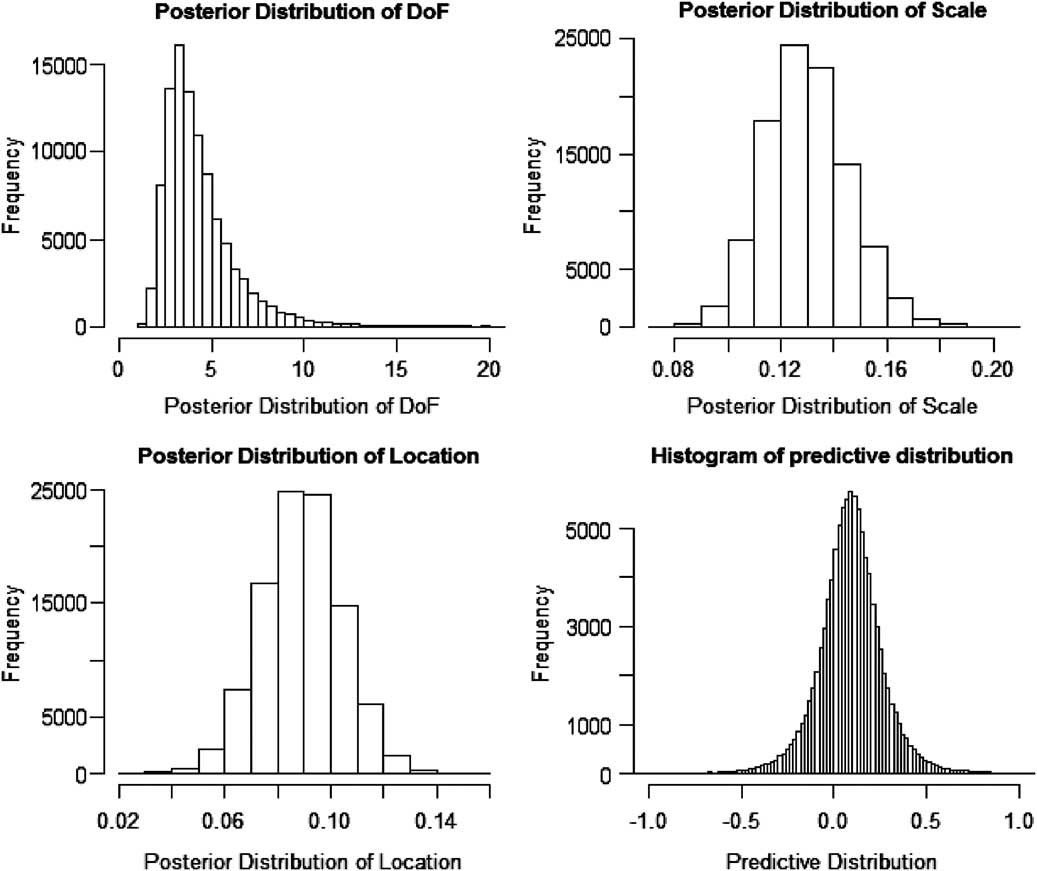
Figure A1 Predictive distribution and posterior distribution for location, scale and degree of freedom
A.9.2.2. Convergence of the MHA
One issue with the MHA is knowing how many simulations to run before a set of stable parameters have been produced. In principle the Markov chains should converge to the limiting distribution, which is the true joint posterior of the model unobservables. There are papers that discuss a number of diagnostic tests that can be used to test whether suitable convergence has been achieved (Cowles & Carlin, Reference Cowles and Carlin1996). For this case study, a simple graphical test was used to observe values of each parameter in each simulation as plotted below (Figure A2).
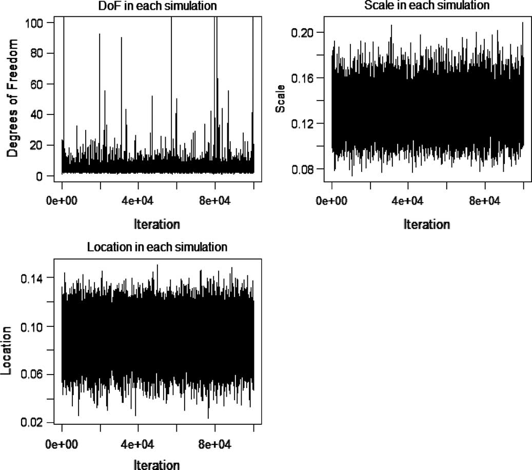
Figure A2 Illustrating the stability of the distribution of for location, scale and degree of freedom
The plots in the graph above show that the values of each parameter have reached a stable distribution and are moving around the sample space of that distribution in each simulation. When running MHAs that are incorrectly specified, these plots would show the parameters diverging in one direction rather than randomly moving around one space.
B Appendix B – Proxy Model Formulae
This appendix is an annex to section 5. It covers the detailed on and details replicating formulae for the following assets and liabilities in section 5.1:
• annuities;
• guaranteed annuities;
• term assurance;
• equities;
• cash, government bonds;
• corporate bonds.
It also covers an example of a smoothing algorithm to remove the bias and sampling error in smoothed percentiles.
B.1. Annuities: Valuation Formula
Assume a constant rate of mortality 1/T in each future year, expressed as a fraction of the initial number of lives, until all have died. The proportion of lives in force at time t is
 $$$\max \left\{ {1\,{\rm{ - }}\,\frac{t}{T},0} \right\}$$$
All policyholders have died by time t = T.
$$$\max \left\{ {1\,{\rm{ - }}\,\frac{t}{T},0} \right\}$$$
All policyholders have died by time t = T.
Thus, the cash flows are (with LCF – liability cash flow per annum before mortality):
 $$${\rm{LCF}}\,(1{\rm{ - 1/}}T)\,{\rm{at}} \ {\rm{the}} \ {\rm{end}} \ {\rm{of}} \ {\rm{year}}\,1$$$
 $$${\rm{LCF}}\,(1{\rm{ - 2/}}T)\,{\rm{at}} \ {\rm{the}} \ {\rm{end}} \ {\rm{of}} \ {\rm{year}}\,2$$$
We use discount rate = risk-free + liquidity premium.
The liability (for unit annual cash flow) is
 $${ &#x0026; PV\, = \,LCF\mathop{\sum}\limits_{t\, = \,1}^{{\rm int}(T)} {\left( {1\,{\rm{ - }}\,\frac{t}{T}} \right){{{(1\, + \,disc)}}^{{\rm{ - }}t}} } \cr &#x0026; \quad\ \ = \,LCF\left\{ {\frac{1}{{disc}} \ {\rm{ - }}\,\frac{{1\, + \,disc}}{{T.dis{{c}^2} }}\left[ {1\,{\rm{ - }}\,\frac{1}{{{{{(1\, + \,disc)}}^{{\rm int}(T)}} }}} \right]\,{\rm{ - }}\,\frac{{1\,{\rm{ - }} \ {\rm int}(T)/T}}{{disc.{{{(1\, + \,disc)}}^{{\rm int}(T)}} }}} \right\} \cr}$$
where int(T) is the integer part of T, that is, the largest integer not exceeding T.
Annuities are single premium products. As the premium has already been paid, we do not need to model it here. There is no lapse risk with annuities.
B.2. Unit Linked with Guarantee: Valuation Formula
We consider a fund with initial value Unit_Fund, invested in risky assets but with a guaranteed amount Gtee_AMT at maturity. We assume that the annual management charge (AMC) is deducted annually in advance. Lapses occur during the year, after the AMC is deducted (with 0 < AMC < 1.00). The total technical provision is the unit fund minus the value of future charges plus the guarantee.
The value of charges is as follows (assuming an integer term T ≥ 1)
 $${ &#x0026; Unit\_Fund \left\lfloor \matrix { AMC\, + \,(1\,{\rm{ - }}\,AMC)(1\,{\rm{ - }}\,lapse)AMC\, + \, \ldots \cr \, + \,AMC{{(1\,{\rm{ - }}\,AMC)}^{T\,{\rm{ - }}\,1}} {{(1\,{\rm{ - }}\,lapse)}^{T\,{\rm{ - }}\,1}} } \right\rfloor \cr &#x0026; = \,Unit\_Fund\,\times \,AMC\frac{{1\,{\rm{ - }} \ {{{(1\,{\rm{ - }}\,AMC)}}^T} {{{(1\,{\rm{ - }}\,lapse)}}^T} }}{{AMC\, + \,lapse\,{\rm{ - }}\,AMC\,\times \,lapse}} \cr}$$
The guarantee is assumed to apply only to policies that reach maturity, and is given by the formula
 $${{(1\,{\rm{ - }}\,lapse)}^T} \,\times \,BS\left( {\frac{{Gtee\_AMT}}{{{{{(1\, + \,disc)}}^T} }},\,{{{(1\,{\rm{ - }}\,AMC)}}^T} \,\times \,Fund,\,volatility\,\times \,\sqrt T } \right)$$
Here, the Black–Scholes formula is
 $${ &#x0026; BS\left( {PVget,PVpay,\alpha } \right)\, = \,PVget\,\times \,\rPhi \left( {\frac{{\ln (PVget/PVpay)}}{\alpha }\, + \,\frac{\alpha }{2}} \right) \cr &#x0026; \qquad \qquad \qquad \qquad \qquad{\rm{ - }}PVpay\,\times \,\rPhi \left( {\frac{{\ln (PVget/PVpay)}}{\alpha } \ {\rm{ - }}\,\frac{\alpha }{2}} \right) \cr}$$
As with the term assurance, we can consider whether the value of the guarantee is more or less than the value of charges. However, we have no simple formula for the breakeven rate of AMC. This is because increasing the charge not only causes a rise in the value of charges (clearly) but also reduces PVpay in the option formula, leading to a rising guarantee cost because more is taken out of the fund before the guarantee is met.
Indeed, in some cases, there is no breakeven management charge, as attempts to increase the value of charges also increase the guarantee cost, with the value of charges never catching up. To avoid this, we have to insist that:
 $$Unit\_Fund\, \gt \,{{{\rm{(1}} \ {\rm{ - }}\,lapse{\rm{)}}}^T} {\rm{/(1}} \ {\rm{ + }}\,disc{{{\rm{)}}}^T} \,\times \,Gtee\_AMT$$
Equivalently, expressing the guarantee as an annual return Gtee_AMT = (1 + gtee_ret) T ×Unit_Fund, a breakeven management charge exists provided the guaranteed return is not too onerous, specifically
 $${\rm{1}} \ {\rm{ + }}\,gtee\_ret\, \lt \,{\rm{(1}} \ {\rm{ + }}\,disc{\rm{)/(1}} \ {\rm{ - }}\,lapse{\rm{)}}$$
As with the term assurance, we can investigate this product on two bases:
• Variant 1 permits negative provisions if charges are sufficiently large: technical provisions = guarantees − charges.
• Variant 2 assumes all policies immediately lapse if provisions were to become negative, so that technical provisions = max{0, guarantees − charges}.
B.3. Term Assurance: Valuation Formula
We assume that lapses are a constant proportion of policies in force during the year, whereas mortality is a constant number of deaths each year (thus, the q-factor increases with age).
We construct the policy count as follows between t−1 and t (Table B1).
Table B1 Evolution of the Term Assurance policy count between times t and t−1

We can then calculate
 $$\openup 6pt{ PVclaims &#x0026; \, = \,SA\mathop{\sum}\limits_{t\, = \,1}^T {\frac{{{{{(1\,{\rm{ - }}\,lapse)}}^{t\,{\rm{ - }}\,1}} \,\times \,mort}}{{{{{(1\, + \,disc)}}^t} }}} = \,\frac{{SA\,\times \,mort}}{{disc\, + \,lapse}}\left\{ {1\,{\rm{ - }} \ {{{\left( {\frac{{1\,{\rm{ - }}\,lapse}}{{1\, + \,disc}}} \right)}}^T} } \right\} \cr}$$
and
 $$\openup 6pt{ &#x0026; PVprems\, = \displaystyle\,annprem\mathop{\sum}\limits_{t\, = \,0}^{T\,{\rm{ - }}\,1} {\frac{{{{{(1\,{\rm{ - }}\,lapse)}}^t} \,\times \,(1\,{\rm{ - }}\,mort\,\times \,t)}}{{{{{(1\, + \,disc)}}^t} }}} \cr &#x0026; = \,\frac{{annprem(1\, + \,disc)}}{{{{{(disc\, + \,lapse)}}^2} }}\left[ \matrix { \left\{ {disc\,{\rm{ - }}\,mort\, + \,lapse\,\times \,mort\, + \,lapse} \right\} \hfill \cr {\rm{ - }}{\displaystyle{\left( {\frac{{1{\rm{ - }}lapse}}{{1\, + \,disc}}} \right)}^T} \left\{ {disc\,{\rm{ - }}\,mort\, + \,lapse\,\times \,mort\, + \,lapse {\rm{ - }}\,(disc\, + \,lapse)\,\times \,mort\,\times \,T} \right\} } \right] \cr}$$
It is easy to find the breakeven premium at which the value of claims is equal to the value of premiums; this occurs when:
 $${ &#x0026; \frac{{breakeven\_annprem}}{{SA}} \cr &#x0026; = \,\frac{\displaystyle{\frac{{mort}}{{disc\, + \,lapse}}\left\{ {1\,{\rm{ - }} \ {{{\left( {\frac{{1\,{\rm{ - }}\,lapse}}{{1\, + \,disc}}} \right)}}^T} } \right\}}}{\displaystyle{\frac{{1\, + \,disc}}{{{{{(disc\, + \,lapse)}}^2} }}\left[ \matrix { \left\{ {disc\,{\rm{ - }}\,mort\, + \,lapse\,\times \,mort\, + \,lapse} \right\} \cr \displaystyle {\rm{ - }}{{\left( {\frac{{1\,{\rm{ - }}\,lapse}}{{1\, + \,disc}}} \right)}^T} \left\{ {disc\,{\rm{ - }}\,mort\, + \,lapse\,\times \,mort\, + \,lapse\,{\rm{ - }}\,(disc\, + \,lapse)\,\times \,mort\,\times \,T} \right\} } \right]}} \cr}$$
We can consider two variants of the valuation formula:
• Variant 1 permits negative provisions if premiums are sufficiently large: technical provisions = PVclaims − Pvprems.
• Variant 2 assumes all policies immediately lapse if provisions were to become negative, so that technical provisions = max{0, PVclaims − Pvprems}
In our example, in the base case, we assume the actual premium is less than the breakeven premium, so that the value of future benefits exceeds future premiums and the technical provisions are positive under Variant 1. This could reflect the situation of a seasoned policy in which mortality was previously higher. However, we make the inequality close enough so that, under the downward mortality stress, the value of benefits is now less than the premiums. This ensures that we obtain different results with Variant 1 and Variant 2.
B.4. Assets
Equities: Responds only to equity stress.
Cash: Unaffected by any stress.
Risk-free bond (term): Affected only by risk-free rate, assuming an annual coupon and term T.
Corporate bond (term): affected by risk-free rate plus credit spread, assuming an annual coupon and term T.
The formula for the risk free bond and corporate bond is
 $${ Market\_Value &#x0026; \, = \,Face\_Value\left\{ {\frac{1}{{{{{(1\, + \,disc)}}^T} }}\, + \,coupon\mathop{\sum}\limits_{t\, = \,1}^T {\frac{1}{{{{{(1\, + \,disc)}}^t} }}} } \right\} \cr &#x0026; = Face\_Value\left\{ {\frac{1}{{{{{(1\, + \,disc)}}^T} }}\, + \,\frac{{coupon}}{{disc}}\left[ {1\,{\rm{ - }}\,\frac{1}{{{{{(1\, + \,disc)}}^T} }}} \right]} \right\} \cr}$$
B.5. Epanechnikov Smoothing of Percentiles
Here we look at logistic Epanechnikov smoothing in a bit more detail. The Epanechnikov kernel function, K(z), and its first derivative are defined by the formula
 $$K(z)\, = \,\left\{ {\displaystyle\matrix {0 &#x0026; \displaystyle{z\,\leq \,{\rm{ - }}1} \cr {\tfrac{1}{2}\, + \,\tfrac{3}{4}z\,{\rm{ - }}\,\tfrac{1}{4}{{z}^3} } &#x0026; {{\rm{ - }}1\,\leq \,z\,\leq \,1} \cr 1 &#x0026; {z\,\geq \,1} } \cr \right ;K^{\prime}(z)\, = \,\left\{ {\matrix{ 0 &#x0026; {z\,\leq \,{\rm{ - }}1} \cr {\tfrac{3}{4} \ {\rm{ - }}\,\tfrac{3}{4}{{z}^2} } &#x0026; {{\rm{ - }}1\,\leq \,z\,\leq \,1} \cr 0 &#x0026; {z\,\geq \,1} \cr } \right.$$
We also define J(z) to be the cumulative distribution function of the logistic distribution, that is
 $$J(z)\, = \,\frac{1}{{1\, + \,{{e}^{{\rm{ - }}z}} }}$$
The idea is to start with the empirical inverse CDF, transform the α-axis to (−∞,∞) using the logistic CDF, smooth the resulting function using the Epanechnikov kernel and then, finally, re-transform the α-axis. Putting these together, we have
 $${{\tilde{F}}^{{\rm{ - }}1}} \left[ {J(y)} \right]\, = \,\mathop{\int}\limits_{{\rm{ - }}\infty }^\infty {{{{\epsilon}}^{{\rm{ - }}1}} K^{\prime}\left( {{{{\epsilon}}^{{\rm{ - }}1}} z} \right){{{\hat{F}}}^{{\rm{ - }}1}} \left[ {J(y\, + \,z)} \right]dz} $$
Here, as before,
 $$${{\hat{F}}^{{\rm{ - }}1}} (\alpha )$$$
is the empirical inverse CDF,
$$${{\hat{F}}^{{\rm{ - }}1}} (\alpha )$$$
is the empirical inverse CDF,
 $$${{\tilde{F}}^{{\rm{ - }}1}} (\alpha )$$$
is the smoothed inverse CDF and ε is a tuning parameter controlling the amount of smoothing. In the limit of ε = 0, there is no smoothing at all; larger values of ε pull more observations into the average. In the other limit as ε tends to infinity, the smoothed inverse CDF corresponds to a point mass at the average of the largest and smallest observations.
$$${{\tilde{F}}^{{\rm{ - }}1}} (\alpha )$$$
is the smoothed inverse CDF and ε is a tuning parameter controlling the amount of smoothing. In the limit of ε = 0, there is no smoothing at all; larger values of ε pull more observations into the average. In the other limit as ε tends to infinity, the smoothed inverse CDF corresponds to a point mass at the average of the largest and smallest observations.
We can break the integral down into a series of integrals over each interval for which the empirical CDF is constant. We can then integrate analytically. This gives the following formula
 $${ {{{\tilde{F}}}^{{\rm{ - }}1}} \left[ {J(y)} \right] &#x0026; \, = \,\mathop{\sum}\limits_{r\, = \,1}^n {\mathop{\int}\limits_{{{J}^{ - 1}} \left( {\frac{{r\,{\rm{ - }}\,1}}{n}} \right){\rm{ - }}y}^{{{J}^{{\rm{ - }}1}} \left( {\frac{r}{n}} \right){\rm{ - }}y} {{{{\epsilon}}^{{\rm{ - }}1}} K^{\prime}\left( {{{{\epsilon}}^{{\rm{ - }}1}} z} \right){{{\hat{F}}}^{{\rm{ - }}1}} \left[ {J(y\, + \,z)} \right]dz} } \cr &#x0026; = \mathop{\sum}\limits_{r\, = \,1}^n {{{X}_{(r)}}\mathop{\int}\limits_{{{J}^{{\rm{ - }}1}} \left( {\frac{{r{\rm{ - }}1}}{n}} \right){\rm{ - }}y}^{{{J}^{{\rm{ - }}1}} \left( {\frac{r}{n}} \right){\rm{ - }}y} {{{{\epsilon}}^{{\rm{ - }}1}} K^{\prime}\left( {{{{\epsilon}}^{{\rm{ - }}1}} z} \right)dz} } \cr &#x0026; = \mathop{\sum}\limits_{r\, = \,1}^n {\left[ {K\left( {\frac{{{{J}^{{\rm{ - }}1}} \left( {\tfrac{r}{n}} \right)\,{\rm{ - }}\,y}}{{\epsilon}}} \right)\,{\rm{ - }}\,K\left( {\frac{{{{J}^{\,{\rm{ - }}\,1}} \left( {\tfrac{{r\, + \,1}}{n}} \right)\,{\rm{ - }}\,y}}{{\epsilon}}} \right)} \right]{{X}_{(r)}}} \cr}$$
The obvious limiting expressions should be used when the arguments of K are infinite. Although our construction used smoothing with an Epanechnikov kernel and logistic transformation, all that really matters are that the functions J and K are valid CDFs. Other distribution functions could equally well have been used.