Methods: models and observational data

Here 16 full ESMs from a total of ~ 60 models from 28 modelling centres whose output has been archived for CMIP5 are analysed. These 16 ESMs span a range of biogeochemical components and pathways. Table I lists the models used in this study, with a reference to their biogeochemical model and an indication of the primary macronutrients that each model simulates. Note that not only do the biogeochemical models vary in their levels of sophistication, but also in the number of nutrients they contain.

As biogeochemistry is a focus here, it is relevant to list the biogeochemical models for reference. There are nine biogeochemical models sampled since CNRM-CM5 (model 4 in Table I) and the IPSL models (11, 12 and 13) use PISCES (Aumont & Bopp Reference Aumont and Bopp2006, Séférian et al. Reference Séférian, Bopp, Gehlen, Orr, Ethé, Cadule, Aumont, Melia, Voldoire and Madec2013). CANESM2 (1) uses CMOC (Zahariev et al. Reference Zahariev, Christian and Denman2008, Christian et al. Reference Christian, Arora, Boer, Curry, Zahariev, Denman, Flato, Lee, Merryfield, Roulet and Scinocca2010), CESM1BGC (2) uses BEC (see Moore et al. Reference Moore, Lindsay, Doney, Long and Misumi2013 and references therein), CMCC-CESM (3) uses PELAGOS (Vichi et al. Reference Vichi, Pinardi and Masina2007), the GFDL models (5 and 6) use TOPAZ2 (see the technical description provided in the supplement to Dunne et al. Reference Dunne, John, Shevliakova, Stouffer, Krasting, Malyshev, Milly, Sentman, Adcroft, Cooke, Dunne, Griffies, Hallberg, Harrison, Levy, Wittenberg, Phillips and Zadeh2013), the GISS models (7 and 8) use NOBM (Gregg Reference Gregg2008), the Hadley Centre models (9 and 10) Diat-HadOCC (Palmer & Totterdell Reference Palmer and Totterdell2001) and the MPI models (14 and 15) HAMOCC5.2 (Ilyina et al. Reference Ilyina, Six, Segschneider, Maier-Reimer, Li and Nez-Riboni2013). The biogeochemical model used in MRI-ESM1 (model 16) is outlined in Adachi et al. (Reference Adachi, Yukimoto, Deushi, Obata, Nakano, Tanaka, Hosaka, Sakami, Yoshimura, Hirabara, Shindo, Tsujino, Mizuta, Yabu, Koshiro, Ose and Kitoh2013), combining their dynamical component MRI.COM3 with a NPZD ecosystem model based on Oschlies (Reference Oschlies2001).

The 16 models have been assessed in terms of their representation of ‘present day climate’ or ‘historical period’, taken to be the period 1976 to 2005 of the model run. This assessment is used to give likelihood estimates on the model future projections under rcp4.5 and rcp8.5, and as a way to construct boundary conditions for downscaling of future states in a high resolution numerical model. At the time of writing the 16 models used had archived most (but not quite all) of the relevant physical and biogeochemical variables for the historical period and for both the rcps that we were able to post-process and analyse. Gaps in model output (in particular associated with the rcps) arise because either the run was never performed, or the relevant model output was never archived.

Figure 1 contours the bathymetry of the Ross Sea region. Within this region a common domain for analysis of observations and model output is shown as the black bounding box. This bounding box has been chosen to capture some of the shelf and deeper waters associated with the Ross Sea gyre, and to avoid inter-model coastline inconsistencies associated with differences in the horizontal spatial resolution between the CMIP5 models, particularly along the front of the Ross Ice Shelf (noting that the present generation of CMIP5 models do not explicitly represent ice shelf processes). We refer to this common domain as region ROSS.

Fig. 1 Colour contour plot of the bathymetry (in metres) of the Ross Sea region (from GEBCO, www.ngdc.noaa.gov/mgg/gebco). The area within the black outline, referred to as region ROSS, is used for the data and model analysis, and spans 171°E to 160°W in longitude and 76°S to 69°S in latitude. Region ROSS samples the Ross Sea continental shelf (< 1000 m) and off-shelf waters (> 1000 m) of the Ross Sea environs. Red contours show isobaths at 1000 and 3000 m.

Figure 2 shows monthly mean averages for November to March over region ROSS of surface chlorophyll (left column) derived from the satellite data averaged over 1997–2005 from the NASA Sea-viewing Wide Field-of-view Sensor (SeaWiFS) instrument (with the white regions missing data), and sea ice concentration (SIC) (right column) from HadISST (Rayner et al. Reference Rayner, Parker, Horton, Folland, Alexander, Rowell, Kent and Kaplan2003) averaged over 1976–2005. According to the supplementary evidence of Pinkerton & Bradford-Grieve (Reference Pinkerton and Bradford-Grieve2010) to the Pinkerton et al. (Reference Pinkerton, Bradford-Grieve and Hanchet2010) paper, there is evidence of satellite underestimate of the in situ chlorophyll in the Ross Sea by ~ 13%, and this is accounted for in the satellite data used here. Further, the range of interannual variation is between 0.4 and 1.6 of each monthly mean estimate, and these values are used as a variance measure around the mean. The ROSS region overlaps with that used by Pinkerton & Bradford-Grieve (Reference Pinkerton and Bradford-Grieve2014), and the present estimates of average surface chlorophyll over the respective domains are similar to those reported in the Pinkerton & Bradford-Grieve (Reference Pinkerton and Bradford-Grieve2010) supplementary evidence.

Fig. 2 Monthly mean surface chlorophyll from SeaWiFS 1997–2005 (mg Chl m^-3, left column) and sea ice concentration (% conc., right column) from HadISST (Rayner et al. Reference Rayner, Parker, Horton, Folland, Alexander, Rowell, Kent and Kaplan2003) for 1976–2005 for November to March over region ROSS (see Fig. 1). Note the non-uniform scale for chlorophyll. Black contour lines show bathymetry at 1000 and 3000 m.

Compared to the surface chlorophyll images from the wider domain in fig. 2 in Smith et al. (Reference Smith, Sedwick, Arrigo, Ainley and Orsi2012), region ROSS misses some of the high intensity signals on the shelf close to the Ross Ice Shelf, but does capture the large amplitude chlorophyll over the shelf break to the east of the domain in December and January. Monthly area averages (not shown) reveal that ROSS matches the timing of the Smith et al. (Reference Smith, Sedwick, Arrigo, Ainley and Orsi2012) domain seasonal cycle, except perhaps underestimating early growth in November, and captures ~ 60% of the total integrated surface chlorophyll.

The HadISST monthly averages for SIC show the emergence of the Ross Sea polynya from November into January, followed by the wider expanse of open water formation in February and the subsequent regrowth from the east and south of region ROSS during March. Compared to fig. 2 in Smith et al. (Reference Smith, Sedwick, Arrigo, Ainley and Orsi2012) it is again apparent that region ROSS is capturing most of the important SIC seasonal signal.

Data representing the historical period are from the World Ocean Atlas (WOA) 2009 database for salinity (Antonov et al. Reference Antonov, Seidov, Boyer, Locarnini, Mishonov, Garcia, Baranova, Zweng and Johnson2010), temperature (Locarnini et al. Reference Locarnini, Mishonov, Antonov, Boyer, Garcia, Baranova, Zweng and Johnson2010), and the nutrients nitrate, phosphate and silicate (Garcia et al. Reference Garcia, Locarnini, Boyer, Antonov, Zweng, Baranova and Johnson2010), and SIC from HadISST (Rayner et al. Reference Rayner, Parker, Horton, Folland, Alexander, Rowell, Kent and Kaplan2003). These sources provide spatial and temporal best fits to in situ observations, and are, therefore, best suited for assessment of climate model output in which we are looking for a statistical comparison of spatial and seasonal patterns averaged over the historical period, rather than a direct match to the individual observations themselves.

For the major circulation factors in the Southern Ocean we consider the Drake Passage transport, and the peak circulation in the sub-polar gyres. Values for the present day Drake Passage transport are obtained from long-term measurements (as indicated by Meijers et al. (Reference Meijers, Shuckburgh, Bruneau, Sallee, Bracegirdle and Wang2012) in their analysis of CMIP5 models in reference to Cunningham et al. (Reference Cunningham, Alderson, King and Brandon2003) and Griesel et al. (Reference Griesel, Mazloff and Gille2012)) spanning a range of 134–164 Sv. The peak sub-polar Ross Sea and Weddell Sea gyre transports are from the Southern Ocean State Estimate (SOSE; Mazloff et al. Reference Mazloff, Heimbach and Wunsch2010) numerical model re-analysis, estimated to be 20 and 40 Sv, respectively.

For an assessment of Intpp there are sparse (in space and time) in situ measurements of primary production in the Ross Sea (see e.g. Pinkerton & Bradford-Grieve Reference Pinkerton and Bradford-Grieve2010 and references therein), but these have typically been used to derive products for global estimates of Intpp. One such product is the so-called vertically generalized production model (VGPM; Behrenfeld & Falkowski Reference Behrenfeld and Falkowski1997), and output from the VGPM has been used here to construct monthly means and standard deviations over region ROSS. Following Pinkerton & Bradford-Grieve (Reference Pinkerton and Bradford-Grieve2010) we adjust the VGPM values by calibration of area averaged surface chlorophyll values, and independent estimates of annual production rates. These adjustments account for the different areas of the Ross Sea over which the estimates are made. In particular Pinkerton & Bradford-Grieve (Reference Pinkerton and Bradford-Grieve2010) use the annual production rate of 140 g C m^-2 y^-1 from Arrigo & van Dijken (Reference Arrigo and van Dijken2004) for the latter’s study area (region AVD, which is largely over the continental shelf). Over the growing season, the satellite data suggests that the ratio of average chlorophyll concentration between regions ROSS and AVD is 0.47, thus we estimate a calibrated annual production over region ROSS to be 66 g C m^-2 y^-1. Over region ROSS, VGPM predicts the annual production to be ~ 55 g C m^-2 y^-1, hence we scale the VGPM values by 1.2 (VGPM*).

Throughout this paper the spatial grids associated with the reference datasets are used as templates for the assessment. Model output is interpolated to the spatial grid associated with the data, and then the relevant statistics are computed. This interpolation can lead to some misrepresentation of the true model coastline, especially where there are relatively large geometrical and spatial differences between the data and model grids. For example, the native horizontal resolution of WOA 2009 is 1° on a regular longitude-latitude grid, while the model grids can have local resolutions smaller or larger, and can be on less standard projections (such as rotated poles etc.). Also, the satellite observations of surface chlorophyll over the Ross Sea contain missing data due to a mixture of low solar elevation, cloud and sea ice (as is apparent in Fig. 2). Any of the computed statistics will be based on the target grid and missing data distribution of the respective reference dataset.

Our statistics are based on area averages, such that the area average A _ave of function A _i , where i labels the grid points within the area, is:

where dS _i is the grid cell area, and the summation is over all grid cells with non-missing data. The results will be presented in terms of area averages of the observed and model values of interest (e.g. temperature, salinity, etc.), the standard deviation of the values of interest (if available), a root-mean-square error (RMSE) measure of the difference between the observed and model values, and a bias (BIAS) taken as (model–observations).

Present day comparisons

From the satellite data, monthly mean area average surface chlorophyll values have been calculated for region ROSS and are plotted on Fig. 3a & b as black circles. Note that the month ordering has been rotated to put the Ross Sea summer months at the middle of the axis. The monthly mean values over the historical period from each of the models are also plotted as the coloured lines. Models 3, 14 and 15 have been plotted in red (model 3 distinguished by a peak shifted to March), the remainder in blue to green. An anomalously low solution associated with model 1 is the dark blue curve. In Fig. 3a the scale accommodates the excess amplitudes predicted by models 14 and 15. The scale is reduced to focus on most of the model solutions in Fig. 3b. Most of the models predict a peak in surface chlorophyll between November and January, with evidence of chlorophyll into April and May beyond that suggested by the light-limited satellite data.

Fig. 3a Satellite (black circles) and individual model monthly mean area averaged surface chlorophyll (mg Chl m^-3). b. Monthly mean area averaged surface chlorophyll (mg Chl m^-3) expanded around satellite data. c. Averaged November to March historical period root-mean-square error (RMSE) (+) and bias (BIAS) (model data) (□) metrics of area averaged surface chlorophyll per model. BIAS greater/less than zero plotted green/blue. The red triangle shows mean model area average surface chlorophyll, the red vertical line shows one standard deviation about the mean. The horizontal dashed line shows the November to March satellite average (0.75 mg Chl m^-3). Inner/outer ensemble and multi-model mean/median ensemble metrics (see text) are labelled I/O and Mn/Md, respectively.

Figure 3c plots the RMSE and BIAS per model (numbered 1–16) averaged over November to March compared to the satellite data. Our assessment of (relative) model skill will consider spatial (over region ROSS) and temporal (over a season) components combined, and so estimation of the time dependence of the spatial errors in terms of RMSE and BIAS represents a potential set of metrics (e.g. see the discussion in Jolliff et al. (Reference Jolliff, Kindle, Shulman, Penta, Friedrichs, Helber and Arnone2009) about alternatives). In this instance, despite the poor solution of model 1, the RMSE and BIAS metrics are not the worst; however, the actual solution of model 1 is the worst as the average value (the red triangle) is well below the data average (the horizontal dashed line). Models 14 and 15 are clear outliers, with excess RMSE and BIAS. Model 3 has a relatively low overall BIAS but not so favourable RMSE, despite its misplaced peak.

Using the RMSE and BIAS from Fig. 3c, we can rank all models for surface chlorophyll. For example, the RMSE value is used to rank the models from 1 to 16, and similarly for the BIAS; the ‘score’ for each model is then simply taken to be the average of its RMSE and BIAS positions, and the lower the overall score the better ranked the model is taken to be. The result of this process is shown in the top frame (labelled ‘Chl’) in Fig. 4. As expected, models 14 and 15 rank the worst, while the relatively anomalous models 1 and 3 rank tenth and ninth, respectively. The next six frames repeat the exercise for SST, the surface nutrients nitrate (NO₃), phosphate (PO₄) and silicate (Si), an estimate of a mixed-layer depth (or depth of the seasonal thermocline, DST), and SIC. A mixed-layer depth is defined to be the depth at which the potential density changes by 0.125 kg m^-3 from its value at the surface (the potential density reconstructed from the monthly mean model values of potential temperature and salinity) and shares properties with the ‘mixed-layer depth’, although given the monthly mean model output timescales is perhaps better associated with a seasonal scale than the relatively rapid dynamics of a ‘mixed-layer depth’ (hence our reference to it as DST). As an indicator of overall performance using the chosen metrics, the bottom frame (‘All’) combines the previous seven rankings by simply summing and averaging each model’s ranking per variable, noting that this mixes physical with biogeochemical variables and models do not all sample the same number of parameters (see the comparably short PO₄ list, for example). This combined ranking shows that models 14 and 15 rank the worst. Therefore, we have defined an initial set of ‘worst fit’ models to form an ‘outer ensemble’ which are models 14 and 15, to which models 1 and 3 are added due to their poor surface chlorophyll representations. The remaining models define an ‘inner ensemble’ of the better ranked models.

Fig. 4 Score and ranking per variable for all models in region ROSS (see Table I). The numbers plotted are the model numbers. Models are ranked by score from lowest (the ‘best’) to highest (‘worst’). ‘All’ combines the scores from all of the other variables to obtain an estimate of an overall ranking.

Examination of the SIC ranking in Fig. 4 reveals that the models split into four approximate groupings. The first group (for the best models) comprises models 5, 8, 1 and 7; these models capture the annual seasonal cycle well, and of these, model 5 captures the February minimum amplitude the best. The annual cycle of area averaged SIC over region ROSS for model 5 is shown in Fig. 5a as the black curve, with the vertical lines indicating the model standard deviation. The HadISST data is shown as the blue circles, with the yellow band the data standard deviation. Apart from slight underestimates in March and April, model 5 matches the data well. Models 2 and 3 form the next group, with good timing of the annual cycle compared to the data (see Fig. 5b for model 2), but neither of these models capture the summer minimum values. Models 10, 9, 11 and 6 form the next group, each typically capturing the February minimum well, but tending to grow too slowly over the autumn period (see Fig. 5c for model 10). The final (worst) group comprises models 4, 12, 15, 14 and 13; these models have too little sea ice over the summer period, and also underestimate the autumn regrowth, typically not matching the data until around July (see Fig. 5d for model 4).

Fig. 5 Examples of model monthly mean sea ice concentration (SIC) for comparison with HadISST for models a. 5, b. 2, c. 10 and d. 4. The black and blue/yellow curves are for model and HadISST monthly mean and variance over the period 1976–2005, respectively.

The monthly mean spatial patterns of SIC for models 5, 2, 10 and 4 are shown in Fig. 6 for comparison with the HadISST data in Fig. 2. In December, model 5 shows a relatively weak Ross Sea polynya emergence in about the right location. In January the opening continues, but tends to spread too far to the east compared to the data, resulting in the relative underestimate in February. The regrowth arises in March with development along the southern part of the domain. For model 2, the Ross Sea polynya emergence and subsequent development matches well the data spatial patterns (in particular the east to west gradient over region ROSS), but as expected the area averaged model amplitude tends to be too high. For model 10, the Ross Sea polynya over region ROSS is not apparent, with the seasonal progression suggesting sea ice thinning at the northern part of the domain. In February and March, model 10 resembles model 5. Finally for model 4, its Ross Sea polynya compares well with the data in December (but perhaps a little underestimated to the east), but clearly has too little ice over region ROSS in January and February, and only a very weak recovery in March.

Fig. 6 Spatial pattern of model monthly mean sea ice concentration for December to March for comparison with HadISST for models 5, 2, 10 and 4.

Note that the rankings for SIC in Fig. 4 reflect both the model temporal and spatial patterns (in Figs 5 & 6, respectively). Consistent with our ‘outer ensemble’ models, 14 and 15 fall into the last grouping for SIC, whereas models 1 and 3 rank relatively well.

The reconstructed surface chlorophyll monthly means from the inner (red) and outer (green) ensembles are shown in Fig. 7. Figure 7a includes the outer ensemble solution, while Fig. 7b does not. For each ensemble the spread about the mean is shown, where the spread is taken to be the average root-mean-square distance between the ensemble members and the ensemble mean. The blue curve with circles shows the mean satellite data, with the yellow band the satellite variance about the mean based on the 0.4 and 1.6 estimates. For comparison, the blue lines are area averaged values obtained from subtracting or adding the monthly mean standard deviation patterns from the SeaWiFS data over the period 1997–2005 to the mean, giving surface chlorophyll lower and upper bound estimates, respectively. The yellow band spans the blue lines, suggesting a consistent measure of the surface chlorophyll interannual variability. In Fig. 7a, the impact of models 14 and 15 to the outer ensemble peak and the shift due to model 3 are clear. In Fig. 7b, it is apparent that the inner ensemble solution matches the data well in terms of the timing with the model spread spanning the data variance, but the ensemble mean is typically in excess of the data mean, at least based on these area average metrics.

Fig. 7 Normalized satellite (blue-yellow), inner ensemble (red), outer ensemble (green), and Mn (black circles) and Md (black triangles) monthly mean area averaged surface chlorophyll (mg Chl m^-3) for region ROSS for a. all models and b. excluding outer ensemble models 3, 14 and 15, and anomalously low model 1. Normalization factor is shown at the top left. The yellow band shows satellite variance about the mean using 0.4 and 1.6 estimates, and the blue lines show satellite variance based on satellite spatial standard deviations per month. Coloured bands for the model ensembles indicate ensemble spread (see text) about ensemble mean.

Also shown in Fig. 7 are the multi-model (using all 16 models) mean (‘Mn’, black circles) and median (‘Md’, black triangles) values. For surface chlorophyll, Mn is typically in excess of the data mean, especially in December and January, whereas Md tracks the data mean very well except for a slight underestimate in October. The respective RMSE and BIAS scores for the inner, outer, and Mn and Md are included in Fig. 3 for comparison with the individual models. The outer and Mn metrics are in excess of the inner and Md equivalents, and as expected Md represents the mean the best (the red triangle), whereas the inner ensemble produces the lowest BIAS score and a relatively lower RMSE value.

The low sample size of 16 models, coupled with the uncertainty regarding the statistical distribution of the model solutions, makes choosing the relevant parametric (or loosely ‘mean-based’) or non-parametric (or loosely ‘median-based’) statistical sampling problematic. The assessment and ranking process for the inner and outer ensembles is both for estimation of the ‘best’ solution and for trying to pick apart why we might need to exclude the outer models from such estimation. For surface chlorophyll the inner solution provides for a working ‘best’ solution (based on our metrics) compared to Mn and Md, and we shall use the inner solution to base assessments of the other variables. However, for reference we shall also provide the Mn and Md values for each variable in the historical data comparisons and also for consideration of model future projections.

Examples of monthly mean surface chlorophyll patterns are presented in Fig. 8 for December to February (from top to bottom). The left column is the satellite data from Fig. 2, the middle column is the inner ensemble, and the right the outer ensemble (noting that the colour scale has been extended to 6.4 mg Chl m^-3 to accommodate the larger outer ensemble amplitudes). For each month the missing data (white) are from the satellite record. For December the inner ensemble (Fig. 8b) captures the elevated band of surface chlorophyll around 75°S in the data (Fig. 8a), with the band extending from the Ross Sea continental shelf, across the shelf break and into the deeper water (the black lines showing the 1000 and 3000 m isobaths). The inner ensemble also captures the northward reduction seen in the data across the continental shelf, with the lower amplitudes arising on the shelf break around 173°E, 71°S. The mean is typically in excess of the data mean but within the variance (see Fig. 7) comprising underestimates along 75°S compared to the data, and overestimates elsewhere, but the spatial pattern is consistent with the data. In comparison, the outer ensemble (Fig. 8c) shows the enhanced chlorophyll signature across most of the shelf, which is even more extensive by January (Fig. 8f) compared to the data (Fig. 8d) and the inner ensemble (Fig. 8e). As before, the inner ensemble tends to underestimate the chlorophyll signature to the south, and overestimate elsewhere, but overall the spatial pattern is consistent with the data and results in the reasonable fit in Fig. 7. By February all three frames (Fig. 8g–i) show a similar average surface chlorophyll amplitude across the entire domain (both on and off the shelf). In fact it might be argued that the outer ensemble (Fig. 8i) is capturing some of the higher chlorophyll signatures in the data across the shelf slope for February better than the inner ensemble, but the metric in Fig. 7 cannot readily distinguish the solutions.

Fig. 8 Reconstructed ensembles from Fig. 7 for December, January and February (rows top to bottom). a., d. & g. Satellite mean, b., e. & h. inner ensemble and c., f. & i. outer ensemble for surface chlorophyll (mg Chl m^-3). Note that the colour scale is extended to 6.4 mg Chl m^-3 compared to the scale in Fig. 2.

Figure 8 provides evidence that the inner models are able to represent the seasonal and spatial surface chlorophyll variations and patterns seen in the data. This suggests that our discrimination on the basis of the metrics used here is enabling a satisfactory fit from the available models. The data contains fine scale features not captured by the models (for example, Fig. 8g shows a number of off-shelf high intensity chlorophyll regions not seen in either of the ensembles), and this is perhaps not surprising given the relatively coarse spatial resolution of the models. Nevertheless, the evidence suggests the inner models are representing some of the important broader scale signatures seen in the data.

Figure 9 compares monthly means, medians and variances for SST (Fig. 9a), SIC (Fig. 9b), the surface macronutrients nitrate (Fig. 9c), phosphate (Fig. 9d), silicate (Fig. 9e) and iron (Fig. 9f), and the integrated (or net) primary production (Fig. 9g). The reference area averages are plotted as blue circles, with yellow bands for the temporal variance where available. As before the inner and outer ensemble means are red and green, respectively, and Mn and Md are the black circles and triangles, respectively. Each graph is normalized to the value at the bottom left of each frame. For SST, the scaling factors are the minimum, maximum and range.

Fig. 9 Normalized area averaged monthly mean plots over region ROSS for a. sea surface temperature (SST), b. sea ice concentration (SIC), c. nitrate (NO₃), d. phosphate (PO₄), e. silicate (Si), f. dissolved iron (DFe) and g. integrated primary production (Intpp) for the historical period. Data are indicated by the blue circles or squares, and the estimated data variance is represented by the yellow band (where available). Inner, outer, Mn and Md ensemble values are shown by red, green, black circles and black triangles, respectively. Normalization factors are shown at the bottom left. For SST the factors are minimum, maximum and range, respectively. Outlier model 3 was removed from the NO₃ and PO₄ outer ensembles, and similarly model 1 for Intpp.

Figure 9a for SST shows that all the ensembles overlap fairly closely over most of the year, except from January to March where the outer ensemble (green) suggests relatively cooler SSTs. Compared to the SST data, the model solutions represent the seasonal cycle well, but overestimate the summer SST peak by ~ 1.5°C (a signature perhaps of the tendency toward a warm bias in the Southern Ocean in CMIP5 coupled models as highlighted in, for example, Wang et al. (Reference Wang, Zhang, Lee, Wu and Mechoso2014)). The lower bounds of the outer ensembles do a better job of approximating the summer SST data, and this is reflected in the good ranking scores for models 1 and 3 in Fig. 4. All ensembles tend not to capture some of the coldest average temperatures seen in the data.

For SIC in Fig. 9b all the ensembles capture the timing of the summer minimum in February, but have the tendency to underestimate the regrowth from March to June seen in the data. The SIC rankings in Fig. 4 show that the outer ensemble models are distributed across the positions and when combined with the different responses illustrated in Fig. 5 result in the range of solutions being blended together.

In Fig. 9c for surface nitrate the anomalously low model 3 solution has been omitted from the outer ensemble. The mean values of each ensemble follow the seasonal cycle and amplitude of the data relatively well, capturing the dip in the December to March period, and returning to similar winter values. However, the spread in the outer ensemble solution is clearly much broader than that of the inner model, perhaps reflecting the comparative spreads in the surface chlorophyll solutions in Fig. 7a, and that the outer ensemble models are ranked the worst for nitrate (see Fig. 4). Further, the inner ensemble spread is relatively narrow, and its mean matches Mn and Md across the seasonal cycle.

For surface phosphate in Fig. 9d the anomalously large model 3 solution has been excluded from the outer ensemble, and also note (see Table I) that model 1 does not include phosphate in its biogeochemical model. The result is a distinct separation between the inner and outer ensembles, with the outer ensemble amplitude lower than the inner ensemble, especially over the summer months. Note that the relatively narrow outer ensemble band presumably results from the outer ensemble models 14 and 15 being from the same modelling centre. Compared to surface nitrate, the phosphate solution for the inner and Md ensembles overlap each other and the data fairly well over the seasonal cycle, but Mn is too large (reflecting the influence of anomalously large model 3 phosphate).

Figure 9e is for surface silicate. Again the inner and outer ensembles are distinct for most of the year, but this time the inner ensemble lies below the outer band, and there is slightly more of an overlap between August to November. As before for surface nitrate, the inner, Md and Mn ensembles match the datapoints remarkably well across the seasonal cycle. Note that the outer ensemble is again only composed of models 14 and 15, as models 1 and 3 do not cycle silicate explicitly in their biogeochemical models.

Note that Smith et al. (Reference Smith, Ainley, Arrigo and Dinniman2014a) observe that the surface macronutrients nitrate, phosphate and silicate are generally not depleted during the phytoplankton growing season, and the inner model solutions are consistent with this picture with proportionately small drops in their values over November to March compared to the rest of the year (see Fig. 9c–e).

The models also predict other less well observed variables of interest biogeochemically. For example, Fig. 9f shows a reconstruction of the monthly mean area average surface iron concentration. Unlike the other nutrients, all the iron ensembles strongly overlap, each ensemble having a seasonal maximum around October and a minimum in January. In the absence of an iron climatology for the oceans, comparison can be made with the in situ data compilation of Tagliabue et al. (Reference Tagliabue, Mtshali, Aumont, Bowie, Klunder, Roychoudhury and Swart2012), in particular their fig. 4c for the upper 100 m iron seasonal cycle for their Ross Sea region (a broad zone spanning 155°W to 180°W and south of 45°S) based on 240 observations over 1990–2008. The median values from fig. 4c are plotted here as the blue circles, and the first and third quartiles provide the yellow band about each value. Figure 9f shows that the models have a summer minimum in January of ~ 2×10^-1 nM, and rising over the year to mean peak values of ~ 7×10^-1 nM in September to October. Apart from February, the data compilation and model amplitudes match reasonably well, even though the respective regions do not overlap too well. However, the models are insistent on a drop in values over the summer, at variance with the observations. Tagliabue et al. (Reference Tagliabue, Mtshali, Aumont, Bowie, Klunder, Roychoudhury and Swart2012) suggest that their elevated February values might be associated with sampling near fast ice melt as opposed to indicating a seasonal trend; they also note that the ‘low throughout the period October to January’ might well signal utilization of winter reserves, which is consistent with the model realization. Also, the model iron is only for the model surface layer (typically ~ 10 m) compared to the upper 100 m values from Tagliabue et al. (Reference Tagliabue, Mtshali, Aumont, Bowie, Klunder, Roychoudhury and Swart2012).

For Intpp (mmol C m^-2 d^-1) in Fig. 9g the anomalously low model 1 has been omitted from the outer ensemble. The blue circles with the yellow variance are the averages from VGPM*, and the blue squares with yellow variance are the values from Pinkerton & Bradford-Grieve (Reference Pinkerton and Bradford-Grieve2010) for their larger domain that also includes the relatively less productive northern waters. In January, the outer ensemble solution (green) has the highest production rate, consistent with the elevated surface chlorophyll in Fig. 7a. Compared to VGPM* all ensemble solutions fall below the November data estimates, but for December to March the inner, Mn and Md solutions compare well. For comparison, the inner ensemble has an average annual production rate for region ROSS of 60.7 g C m^-2 y^-1 underestimating the 66 and 85 g C m^-2 y^-1 from VGPM* and Pinkerton & Bradford-Grieve (Reference Pinkerton and Bradford-Grieve2010), respectively.

If the conditions determining the wider circulation in the ROSS region are relevant to the biogeochemical outcomes (and presumably they are) then Fig. 10a & b rank the models based on major circulation characteristics in the Southern Ocean, viz the transport in the Antarctic Circumpolar Current (ACC), and the peak transports in the Ross and Weddell Sea sub-polar gyres, with the individual ranked transports plotted as the blue symbols A, R and W, respectively. Best observational estimates of the Drake Passage (ACC) transport, and the peak Ross and Weddell gyre transports are centred around (149, 20, 40) Sv, respectively. Figure 10a shows the ranking of each model per transport measure, and the black circle indicates an overall score based on the radial distance from the observed values. Figure 10b takes the overall scores and now plots the individual models in rank order. The higher the location of a symbol or the black circle, the lower the confidence in the model estimate relative to the other models in the sample. In this case, Fig. 10b shows that model 2 provides the relatively best combined estimates of the transport values, and model 8 relatively the worst; the A/R/W rankings are clustered around low ranking values for model 2, whereas model 8 has a moderate ranking for W, but equal worst values for A and R. Model 1 from the outer ensemble actually ranks well, whereas models 14 and 15 are at the lower end.

Fig. 10a c. & e. Variable rankings per model and overall score (black circles), with respective ordered overall ranking in b., d. & f. using 1976–2005 averages. Model number is plotted on b., d. & f. Symbols A, R and W show Drake Passage transport, peak Ross Sea gyre transport and peak Weddell Sea gyre transport rankings, respectively. Symbols C, T, N, P, S, D and I label surface chlorophyll, sea surface temperature, nitrate, phosphate and silicate, depth of the seasonal thermocline, and sea ice concentration, respectively, for root-mean-square error (RMSE) (red) and bias (BIAS) (green) rankings.

Figure 10c shows the rankings based on the RMSE (in red) and BIAS (in green) scores for the surface chlorophyll (C), temperature (T), nitrate (N), phosphate (P), silicate (S), DST (D) and SIC (I). It is these individual rankings per variable that were used to obtain Fig. 4. The RMSE ranking per variable is plotted to the left of the vertical dotted line locating each individual model, the BIAS ranking to the right, with the black circle on the line the overall model score as before. The overall score is based on taking equal contributions from each variable. Based on this combination of metrics, model 16 ranks well for nitrate, phosphate and DST, relatively poorly for the chlorophyll bias (in green), but overall ranks the best (although note that this model does not explicitly cycle silicate or iron biogeochemically). In contrast, model 1, that only cycles nitrate, scores poorly for the biogeochemical components chlorophyll and nitrate, and thus ranks as one of the weaker overall models. Models 14 and 15 rank the lowest in Fig. 10d, and model 3 is in the outer ensemble as a result of its poor seasonal solution for surface chlorophyll (see Fig. 3), even though its ranking scores for SST and DST are relatively good.

Comparing Fig. 10b and 10d a degree of overlap between the relative ranking of each model is apparent, e.g. models 8, 14 and 15 rank poorly in both and suggest a potential link between the wider dynamics and the processes in the Ross Sea. However, this does not explain all the rankings, e.g. models 1 and 16 swap their relative rankings between these frames. The transport estimates in Fig. 10a can be combined with the variables in Fig. 10c to produce the ranking shown in Fig. 10e. As before, each variable is assumed to contribute equally to the overall score. This combined ranking confirms that indeed the biogeochemical outcomes of models 14 and 15 are probably influenced by their relatively poor representation of the large scale circulation, and as Fig. 10a shows it is not their ACC transport that scales poorly but rather the individual strengths of each of the sub-polar gyres relative to the other models. On the other hand, the dynamical solution of model 1 is relatively good; therefore, perhaps in this case it is the biogeochemical model that leads to relatively poor outcomes for region ROSS. Comparing Fig. 10b and 10d it is apparent that the model ranking based on the transport estimates alone (Fig. 10b) separates the model ranking scores more widely than the relatively mixed physical and biogeochemical rankings (Fig. 10d). In terms of the combined estimate in Fig. 10f, it is perhaps not surprising that models 8, 14 and 15 are the least well ranked models. Models 1 and 3 end up with combined rankings that place them toward the weaker end of the ranking. Note that the equal weighting per variable means that the wider spread in Fig. 10b is flattened somewhat by the relatively more even spread of Fig. 10d.

Based on Fig. 10 and the preceding analyses, the separation of the CMIP5 models into inner and outer ensembles seems to have a degree of consistency. In developing potential future physical and biogeochemical downscaling for region ROSS, we would consider excluding the outer models 3, 14 and 15, and model 1 due to its anomalously low surface chlorophyll, and use the remaining models comprising the inner ensemble. The metrics of RMSE and BIAS applied to area averaged satellite chlorophyll estimates and surface nutrients from WOA 2009 show that the inner ensemble is able to capture the seasonal cycle rather well in both phase and amplitude. This consistency also applies to the Intpp values compared to the derived primary production estimates that capture the phase well but perhaps underestimate the total production. Surface iron and SIC both show a degree of overlap between their respective ensembles. Such an assessment is useful as it allows a measure of confidence to be applied to the model results, especially when considering model reconstructions of relatively unobserved parameters (such as Intpp and surface iron).

Another dynamical issue associated with CMIP5 model representation of the Antarctic gyres has been recently documented by Heuzé et al. (Reference Heuzé, Heywood, Stevens and Ridley2013). Bottom water formation around Antarctica for the present day is associated with dense water creation on the continental shelves that is then exported via shelf overflows to the lowest levels of the Southern Ocean. The analysis of Heuzé et al. (Reference Heuzé, Heywood, Stevens and Ridley2013) finds that 10 of the 15 CMIP5 models do indeed generate dense water on the shelf but that this water is not exported to depth, i.e. none of the models analysed generate Southern Ocean bottom water in the expected manner. Around half of the models actually generate bottom water via in situ convection events rather than the advective pathway occurring in nature. Furthermore, some of these models have relatively extensive convection zones which seem to result in strong sea ice seasonality, so that there appear to be dynamical ramifications of this anomalous process. Any process that exaggerates the seasonality is likely to impact the biogeochemical response; in that context we examine the rankings we have obtained in the light of the Heuzé et al. (Reference Heuzé, Heywood, Stevens and Ridley2013) results.

From figs 1 and 2 in Heuzé et al. (Reference Heuzé, Heywood, Stevens and Ridley2013), the models that overlap with our study are 1, 4, 5, 6, 8, 10, 11 and 14. Using their metrics, models 1, 5, 10, 11 and 14 are found to have an acceptable bottom temperature representation compared to present day climatology, while models 1, 5, 8, 10 and 14 do likewise for bottom density. However, Heuzé et al. (Reference Heuzé, Heywood, Stevens and Ridley2013) note that models 5, 6 and 8 have extensive areas of deep convection, while models 10, 11 and 14 exhibit this convection only within the sub-polar gyres. Model 4 has no apparent deep convection resulting in too light dense water; model 1 behaves similarly, but nevertheless seems to support deep water of about the right properties. It is apparent that our choice of inner and outer ensembles cannot simply be explained on the basis of the dynamical properties detailed by Heuzé et al. (Reference Heuzé, Heywood, Stevens and Ridley2013), mirroring the earlier consideration of the ACC and gyre transports.

As an example of the potential impact, Fig. 11 plots the logarithm of the monthly mean area averaged DST for region ROSS. In comparison to the data (in blue), all ensembles have significantly larger depths from June to November, and underestimates compared to the data from December to March, but each accurately captures the timing of the summer minimum in January. The spread in model solutions is also large, particularly for the inner ensemble (in red) from April to November. The individual models 8, 9, 10, 11 and 12 from the inner ensemble, and models 14 and 15 from the outer ensemble have maximum DSTs in excess of 800 m; if we consider these models as DST outliers and exclude each from their respective ensembles we get the solutions shown in Fig. 11b. Now the model variance in both the inner and outer ensembles is reduced over winter, and their mean values are much closer to the data in October to November and May to June. In the summer, the reduced outer ensemble now more accurately tracks the data compared to the inner, Mn and Md which remain relatively low over this period.

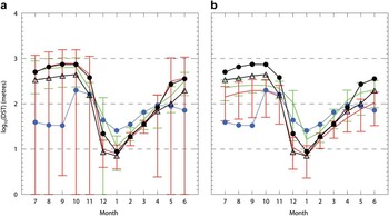
Fig. 11 Ensemble reconstruction for inner (red), outer (green), and Mn (black circles) and Md (black triangles) of monthly mean area averaged depth of the seasonal thermocline (DST) in metres (plotted logarithmically) for region ROSS. Data values are shown as blue circles. a. Includes all models, while b. excludes models 14 and 15 from the outer ensemble, and models 8, 9, 10, 11 and 12 from the inner ensemble.

In comparison with the properties discussed by Heuzé et al. (Reference Heuzé, Heywood, Stevens and Ridley2013), our DST outlier models 10, 11 and 14 overlap in terms of their DST perhaps capturing deep convection within the sub-polar gyres. Models 5 and 6 have extensive convection regions, but not over region ROSS, whereas model 8 does, hence a DST outlier. Also, models 1 and 4 are not excluded, consistent with not being DST outliers. On this basis, models 14 and 15 might point to their inclusion in the outer ensemble because of these convective events; however, this is clearly not the complete explanation for model 1. Therefore, a metric based on the Heuzé et al. (Reference Heuzé, Heywood, Stevens and Ridley2013) results does not uniquely determine a best-fit biogeochemical ensemble for region ROSS. The reason may simply be that potentially anomalous DST dynamics in the winter do not have a detrimental impact on the summer biogeochemical growth, and are perhaps associated with the relatively narrow range of DST solutions obtained by all of the models in summer.

Model projections

Given some confidence intervals on the model solutions for the ‘present day’, it is possible to look at future predictions based on the so-called rcp scenarios associated with the IPCC 5th Assessment Round (AR5). Here rcp4.5 and rcp8.5 are examined for their changes relative to the present day means for averages over the periods 2036–2055 and 2081–2100, such that projections 1 and 2 are for rcp4.5 for 2036–2055 and 2081–2100, and projections 3 and 4 are for rcp8.5 for 2036–2055 and 2081–2100, respectively. Examples of such future predictions are plotted in Fig. 12 for the area average changes over region ROSS relative to the present day. Inner and outer models are shown in red and green, respectively, with each individual model number labelled. The inner and outer ensemble average changes are shown by the red and green circles, respectively, and the black circles and triangles show the respective changes in Mn and Md. Individual model numbers have been spread horizontally to make them more readable, and vertical dotted lines separate the different projections.

Fig. 12 Model projections 1, 2, 3 and 4 (see text) for region ROSS for changes in a. sea surface temperature (SST), b. depth of the seasonal thermocline (DST), c. sea ice concentration (SIC), d. surface chlorophyll, e. integrated primary production (Intpp), f. dissolved iron (DFe), g. nitrate (NO₃), h. phosphate (PO₄), i. silicate (Si) relative to model historical average. Red/green indicates inner/outer models, the symbols represent individual model values and the circles represent ensemble averages. Black circles/triangles show Mn/Md changes, respectively. Symbols left of each DST centreline show reduced model sets (see text). Vertical dashes separate projections. Horizontal dashes locate zero change. T and K show the 95% confidence level significance for Student’s t-test and Kolmogorov-Smirnov test, respectively.

Along the bottom of each frame in Fig. 12 there are symbols ‘T’ and ‘K’ plotted for each projection. The presence of T shows that the distribution of all of the model changes for that projection lead to a mean that is different from zero at the 95% confidence level based on the two-sided Student’s t-test. The presence of K shows that > 50% of the individual model interannual 20 year time series over the projection period differs from that model’s interannual 30 year time series over the historical period at the 95% confidence level based on the two-sample Kolmogorov-Smirnov (K-S) statistical test. The K-S test is used here to give a measure of how distinct the respective interannual time series are, and 50% is arbitrarily chosen to flag that there are indeed a proportion of the samples contributing to the overall mean that are measurably distinct.

For the SST changes in Fig. 12a it is clear that (apart from model 4 that suggests quite large SST changes, and model 5 which has reductions in SST for projections 1 to 3) the ensemble averages actually predict quite similar outcomes, in particular something like a 0.15°C annual average SST rise by the end of the century for projections 1 to 3, with 0.3 and 0.4°C rises for projection 4 for Md and Mn, respectively. All projections are labelled with T, and 1 and 4 with K, showing a good degree of statistical significance.

For DST in Fig. 12b the mean annual values down the projection centreline use the full ensembles, while those to the left of each centreline are based on reduced ensembles from eliminating models with excessive convection. In all cases there is considerable shallowing of DST. For the full ensemble there are decreases of ~ 50–70 m over projections 1 to 3, with decreases of between 90 and 190 m for projection 4. For the reduced ensembles the changes remain significant but smaller, ranging between 70 and 130 m of shallowing. Note that all projections pass the Student’s t-test (and are labelled with T). Note that for DST we have not presently reconstructed the full annual time series using the annual average three dimensional values of temperature and salinity, hence cannot yet ascribe a K confidence level.

The SIC changes in Fig. 12c have a similar pattern to DST, with projections 1 to 3 showing annual average reductions of 2–7%, with the reduction rising to 8–11% for the ensemble means for projection 4. Again all projections are labelled with T and projection 4 with K. Note that model 4 has excessive reductions in concentration consistent with the projected changes in SST.

In comparison, Fig. 12d for surface chlorophyll shows a relatively distinct separation between the inner and outer ensemble projections, with the outer ensemble suggesting increases of ~ 0.18 mg Chl m^-3 by the end of the century compared to much smaller increases from the inner ensemble of ~ 0.04 mg Chl m^-3 (with some of the inner ensemble models predicting a potential fall). These contrast with the annual average value of ~ 0.31 mg Chl m^-3 for the present day (see Fig. 7). The overall average suggests increases in surface chlorophyll in the future, most significantly for projection 4.

Figure 12e for changes in Intpp shows another broad spread in model solutions, with both sets of ensemble members generally showing increases of Intpp for each projection, although there are some predicting future decreases. By the end of the century both averages of the ensembles predict annual Intpp increases of ~ 1.7 mmol C m^-2 d^-1 compared to the annual average derived for the present day (see Fig. 9g) of ~ 16.0 mmol C m^-2 d^-1. Consistent with the surface chlorophyll changes, Intpp is most significant for projection 4.

The individual model solutions for surface iron in Fig. 12f show a broad spread in predicted changes. As a result, only projection 2 passes the t-test to suggest changes statistically different from zero, and in this case the average increase is 0.03 nM compared to the present day model average of ~ 0.325 nM. In comparison, the changes in the surface macronutrients nitrate, phosphate and silicate in Fig. 12g, h & i, respectively, show a general decline toward the end of the century, with the falls in the inner ensemble average values larger than those of the outer ensemble (especially for model 13). In particular for projection 4, the surface nitrate, phosphate and silicate fall by ~ 2, 0.1 and 5 mmol m^-3 compared to present day annual averages of 26.4, 1.8 and 60.2 mmol m^-3 (from Fig. 9c–e), respectively. Note that phosphate passes the K-S test for each projection, but not the Student’s t-test, whereas the nitrate and silicate changes are significant over nearly all projections.

The projection 4 changes based on the ensemble mean (the black circles in Fig. 12) are summarized in Table II as the annual means. The seasonal means are based on November to March over the growing season. Also listed are the respective means from the data, and the percentage change over projection 4 compared to the data mean. The DST changes are from the reduced ensembles that eliminate the excessive convection models, since the latter models are generally found to stop convecting over this period (see De Lavergne et al. Reference De Lavergne, Palter, Galbraith, Bernardello and Marinov2014) and provide exaggerated changes relative to present day. The overall picture is of significant area averaged warming over region ROSS, consistent with decreases in sea ice cover and DST (hence increased stratification). The biological response is an area averaged increase in surface chlorophyll and Intpp, accompanied by reductions in surface nitrate, phosphate and silicate, and relatively smaller increases in surface iron.

Summary

Using metrics based on area averages over a region covering the Ross Sea sector of the Southern Ocean (referred to as region ROSS), a consideration of the biogeochemical outcomes of 16 CMIP5 models has been made compared to present day observations. The consideration suggests that we can split the models into an inner and outer ensemble based on their general representation of the observations (where the inner ensemble models provide for a measurably better fit to the data, in this case with a focus on the surface chlorophyll, compared to the outer ensemble models). Models MPI-ESM-LR (14) and MPI-ESM-MR (15) perform relatively poorly overall compared to all the other models for region ROSS, model CANESM2 (1) is the next poorest in the overall ranking (with an anomalously low amplitude of surface chlorophyll and consequently low Intpp), while model CMCC-CESM (3) generates anomalously large surface phosphate, low nitrate and has a shifted peak in surface chlorophyll. These models 1, 3, 14 and 15 are, therefore, referred to as our outer ensemble.

The selection of these ensembles clearly separates the solutions for the surface chlorophyll and the surface nutrients nitrate, phosphate and silicate; the inner ensembles overlap the observations in amplitude and phase, whereas the outer ensembles tend to be clearly either too high or too low. For surface iron, the ensemble solutions tend to overlap each other with comparable seasonal cycles, whereas for the Intpp the outer ensemble again overestimates in comparison to the derived estimates (perhaps consistent with the model surface chlorophyll solutions). For many of the variables analysed, the mean inner model solution overlaps the multi-model median solution; however, this is not as clear for surface chlorophyll, and times in the seasonal cycle where the solutions diverge for the DST and Intpp.

Comparison with larger scale dynamical properties of the sub-polar gyres suggests that there is no single answer that explains the split into our inner and outer ensembles. Certainly models MPI-ESM-LR (14) and MPI-ESM-MR (15) produce sub-polar gyral transports in excess of many of the other models, which may explain their relatively poor overall performance. However, this is not apparent for models CANESM2 (1) and CMCC-CESM (3), so it may fall to the nature of their specific biogeochemical models rather than purely dynamics. This is also true for the recent analysis by Heuzé et al. (Reference Heuzé, Heywood, Stevens and Ridley2013) looking at the model generation of bottom water; poor performance can partly explain our ensemble choice, but not completely. Indeed, our analysis of DST in region ROSS shows that anomalous DST models overlap the inner and outer ensembles, so again it would appear no single factor is at play in discriminating the models.

This is also true for the SIC comparisons, with members of the outer ensemble distributed right across the rankings. Recent papers have examined the broader Antarctic sea ice representation in the CMIP5 models, in particular Turner et al. (Reference Turner, Bracegirdle, Phillips, Marshall and Hosking2013) and Shu et al. (Reference Shu, Song and Qiao2015). The general conclusion is that the models do a generally poor job of realizing the satellite observations of SIC over the historical period, with nearly all the models showing a decreasing trend in SIC at variance with the observations. Shu et al. (Reference Shu, Song and Qiao2015) expand the 18 models studied by Turner et al. (Reference Turner, Bracegirdle, Phillips, Marshall and Hosking2013) to encompass 49 of the CMIP5 models, and come to much the same conclusions regarding SIC, but do find that some of the models are able to capture observed trends in sea ice extent (SIE) and volume (SIV) over the satellite period. The models that Shu et al. (Reference Shu, Song and Qiao2015) found to perform best from our sample are 3, 8, 12, 13 and 15 for SIE, and 3, 12, 13 and 15 for SIV. A comparison with our SIC regional rankings in Fig. 4 shows models 3 and 8 performing relatively well, but models 12, 13 and 15 not so. On this basis, the dynamical link between the broader Antarctic sea ice representation and the other variables is not immediately apparent. This does not mean, of course, that there is not a link, rather the present analysis and set of metrics is not able to reveal it.

On average the ensembles predict an increase in surface temperature over region ROSS by the end of the century, with smaller relative increases in surface chlorophyll and potentially larger relative increases in Intpp based on rcp4.5 and rcp8.5. For surface chlorophyll and Intpp, the average ensemble solutions do tend to separate, with the outer ensemble projected changes typically larger than those of the inner ensemble. There are also significant reductions in SIC and DST over this period.

However, the model generation of open ocean convection in the Southern Ocean models described by Heuzé et al. (Reference Heuzé, Heywood, Stevens and Ridley2013) certainly complicates the analysis of predictive skill from the CMIP5 models. As has recently been highlighted by Stössel et al. (Reference Stössel, Notz, Haumann, Haak, Jungclaus and Mikolajewicz2015), models are sensitive to the distribution of freshwater over the Southern Ocean (in particular in enabling model behaviour to transition from convecting to non-convecting), consolidating similar results found in the studies of Martin et al. (Reference Martin, Park and Latif2013) and Pierce et al. (Reference Pierce, Barnett and Mikolajewicz1995), for example. Stössel et al. (Reference Stössel, Notz, Haumann, Haak, Jungclaus and Mikolajewicz2015) found that improved ACC transport in their model was also probably linked to changes in the Southern Ocean density and meridional density gradients (again with reference to the work of Martin et al. (Reference Martin, Park and Latif2013) and Pierce et al. (Reference Pierce, Barnett and Mikolajewicz1995)). Furthermore, the analysis of future CMIP5 model pathways by De Lavergne et al. (Reference De Lavergne, Palter, Galbraith, Bernardello and Marinov2014) suggests that models described by Heuzé et al. (Reference Heuzé, Heywood, Stevens and Ridley2013) that are deemed convecting for the historical period will actually transition to non-convecting mode under rcp8.5. Our results, while not attributing any specific cause, certainly show how such competition between modelled Southern Ocean processes is consistent with a wide spectrum of CMIP5 model responses.

An assessment of this sort is generally focused around a particular outcome, in this case the seasonal biogeochemical response. However, the complete solution is of course ‘coupled’ via all the dynamical variables that drive the system (and more so for a polar region such as the Ross Sea because of the direct cryospheric influences such as sea ice, ice shelves, etc.). Thus in reality the production of a ‘best’ ensemble solution will require a broader inclusion of forcing influences. Nevertheless, the assessment here shows that separation into inner and outer biogeochemical ensembles can result in a consistent solution compared to the observations within the biogeochemical context (and some of the dynamical constraints). This discrimination is then useful in assessing both less well observed present day variables (e.g. in situ iron and Intpp), and placing confidence levels on future projections. Bopp et al. (Reference Bopp, Resplandy, Orr, Doney, Dunne, Gehlen, Halloran, Heinze, Ilyina, Seferian, Tjiputra and Vichi2013) in their conclusions urge continuation of inter-model comparisons such as these due to the high uncertainties in model projections, as well as signalling caution when attempting downscaling with single CMIP5 model outputs. This study is intended to progress such work, and although we may not be able to explain the processes resulting in our choices and conclusions, the results as we have them are useful in providing guidance on the quality of the regional solutions from the CMIP5 models for the Ross Sea.