1. Introduction
In the classical compound Poisson risk model, the surplus process ![]() $\left\{ {U_{{\asterisk}} \left( t \right)} \right\}_{t} _{{\geq 0}} $
of a single line of insurance business is modelled by
$\left\{ {U_{{\asterisk}} \left( t \right)} \right\}_{t} _{{\geq 0}} $
of a single line of insurance business is modelled by
where u≥0 is the insurer’s initial surplus, c>0 the constant premium income per unit time, {N(t)}t≥0 a counting process that counts the number of claims and X n the size (or severity) of the n th claim. It is assumed that {N(t)}t≥0 is a Poisson process with rate λ>0, and ![]() $$\{ X_{n} \} _{{n\,=\,1}}^{\infty} $$
is a sequence of independent and identically distributed (i.i.d.) random variables independent of {N(t)}t≥0. The time of ruin of the process
$$\{ X_{n} \} _{{n\,=\,1}}^{\infty} $$
is a sequence of independent and identically distributed (i.i.d.) random variables independent of {N(t)}t≥0. The time of ruin of the process ![]() $\left\{ {U_{{\asterisk}} \left( t \right)} \right\}_{t} _{{\geq 0}} $
is defined by
$\left\{ {U_{{\asterisk}} \left( t \right)} \right\}_{t} _{{\geq 0}} $
is defined by ![]() $$T_{{\asterisk}} ={\rm inf}\{ t\geq 0:U_{{\asterisk}} (t)\,\lt \,0\} $$
, which is the first time that the surplus process drops below zero. One requires the positive security loading condition c>λE[X 1] to ensure that the event of ruin
$$T_{{\asterisk}} ={\rm inf}\{ t\geq 0:U_{{\asterisk}} (t)\,\lt \,0\} $$
, which is the first time that the surplus process drops below zero. One requires the positive security loading condition c>λE[X 1] to ensure that the event of ruin ![]() $\{ T_{{\asterisk}} \,\lt \,\infty\} $
is not certain.
$\{ T_{{\asterisk}} \,\lt \,\infty\} $
is not certain.
A drawback of the above model is that the surplus process ![]() $\left\{ {U_{{\asterisk}} \left( t \right)} \right\}_{t} _{{\geq 0}} $
will grow to infinity in the long run, which leads to the idea of redistributing some of the surplus to the shareholders of the insurance company (de Finetti, Reference de Finetti1957). One of the most commonly studied dividend strategies is the barrier strategy (see e.g. Gerber, Reference Gerber1979; Lin et al., Reference Lin, Willmot and Drekic2003; Dickson & Waters, Reference Dickson and Waters2004; Gerber et al., Reference Gerber, Shiu and Smith2006), in which the entire incoming premium rate is paid to the shareholders as dividend immediately whenever the surplus reaches a fixed barrier level b (as long as ruin has not occurred). Mathematically, the modified surplus process {U(t)}t≥0 with U(0)=u≥0 and u≤b can be described by
$\left\{ {U_{{\asterisk}} \left( t \right)} \right\}_{t} _{{\geq 0}} $
will grow to infinity in the long run, which leads to the idea of redistributing some of the surplus to the shareholders of the insurance company (de Finetti, Reference de Finetti1957). One of the most commonly studied dividend strategies is the barrier strategy (see e.g. Gerber, Reference Gerber1979; Lin et al., Reference Lin, Willmot and Drekic2003; Dickson & Waters, Reference Dickson and Waters2004; Gerber et al., Reference Gerber, Shiu and Smith2006), in which the entire incoming premium rate is paid to the shareholders as dividend immediately whenever the surplus reaches a fixed barrier level b (as long as ruin has not occurred). Mathematically, the modified surplus process {U(t)}t≥0 with U(0)=u≥0 and u≤b can be described by
The quantities of interest in the literature include the Gerber−Shiu expected discounted penalty function (Gerber & Shiu, Reference Gerber and Shiu1998) and the expectation or even the higher moments of the discounted dividends payable until ruin (Dickson & Waters, Reference Dickson and Waters2004). The study of barrier strategy is of great importance because it is known to be optimal in maximising the expected discounted dividends until ruin when the density of X 1 is completely monotone (e.g. Loeffen, Reference Loeffen2008, Theorem 3). In addition, for any given claim distributions, the optimal dividend barrier is independent of the initial surplus level. We refer interested readers to Albrecher & Thonhauser (Reference Albrecher and Thonhauser2009) and Avanzi (Reference Avanzi2009) for comprehensive reviews of different dividend strategies and related optimality results in the literature.
Recently, there has been increased interest in multi-dimensional risk theory in which the surplus processes of more than one line of business are jointly analysed. In multi-dimensional risk models, the frequencies and/or the severities of insurance claims payable by different insurers are generally correlated. Practically, such a situation arises when the insurers are subject to “common shocks” as a result of catastrophic events (e.g. earthquakes and tsunamis) inducing large and correlated claims to them at the same time, or when an insurer transfers part of its claims to one or more reinsurers via a reinsurance contract. In this paper, we follow the former formulation, although applications to the latter situation are also possible (see Remark 1 and section 3.3). We shall consider two lines of business, and each of them implements a dividend barrier strategy. The bivariate surplus process {(U 1(t), U 2(t))}t≥0 with initial surplus levels (u 1, u 2)=(U 1(0), U 2(0)) and dividend barriers (b 1, b 2) (where 0≤u 1≤b 1 and 0≤u 2≤b 2) is described by, for k=1, 2:
 $$dU_{k} (t)=\left\{ {\matrix{ {c_{k} \:dt\,{\minus}\,d\left( {\mathop{\sum}\nolimits_{n\,=\,1}^{N_{{kk}} (t)} {Y_{{k,n}} } {\plus}\mathop{\sum}\nolimits_{n\,=\,1}^{N_{{12}} (t)} {Z_{{k,n}} } } \right),} & {0\leq U_{k} (t)\,\lt \,b_{k} } \cr {{\minus}\,d\left( {\mathop{\sum}\nolimits_{n\,=\,1}^{N_{{kk}} (t)} {Y_{{k,n}} } {\plus}\mathop{\sum}\nolimits_{n\,=\,1}^{N_{{12}} (t)} {Z_{{k,n}} } } \right),} & {U_{k} (t)=b_{k} } \cr } } \right.$$
where (c 1, c 2) are the premium rates of the two lines, and {N 11(t)}t≥0, {N 22(t)}t≥0 and {N 12(t)}t≥0 are mutually independent Poisson processes with respective parameters λ 11, λ 22 and λ 12. Furthermore, ![]() $$\{ Y_{{1,n}} \} _{{n\,=\,1}}^{\infty} ,\,\{ Y_{{2,n}} \} _{{n\,=\,1}}^{\infty} \,{\rm and}\,\,\{ (Z_{{1,n}} ,Z_{{2,n}} )\} _{{n\,=\,1}}^{\infty} $$
are mutually independent i.i.d. sequences, independent of the above three Poisson processes and distributed as the generic random variables Y 1, Y 2 and (Z 1, Z 2), respectively. For each k=1, 2, the process {N kk(t)}t≥0 counts the number of claims faced by the k th business only for claims that arise from the “usual” claim occurrences with severity distributed as Y k. On the other hand, {N 12(t)}t≥0 counts the number of “common shocks” that result in possibly dependent claims distributed as (Z 1, Z 2) to the two lines. It is assumed that Y 1, Y 2 and (Z 1, Z 2) are all positive continuous random variables with cumulative distribution functions (cdfs) F 11(·), F 22(·) and F 12(·,·), respectively. It will be convenient to present F 12(·,·) in copula form (e.g. Nelsen, Reference Nelsen2006) as F 12(z 1, z 2)=C(F 1∙(z 1), F ∙2(z 2)), where C(·,·) is a copula and F 1∙(z 1) and F ∙2(z 2) are the marginal cdfs of Z 1 and Z 2, respectively. For later use we also define the probability density functions (pdfs)
$$\{ Y_{{1,n}} \} _{{n\,=\,1}}^{\infty} ,\,\{ Y_{{2,n}} \} _{{n\,=\,1}}^{\infty} \,{\rm and}\,\,\{ (Z_{{1,n}} ,Z_{{2,n}} )\} _{{n\,=\,1}}^{\infty} $$
are mutually independent i.i.d. sequences, independent of the above three Poisson processes and distributed as the generic random variables Y 1, Y 2 and (Z 1, Z 2), respectively. For each k=1, 2, the process {N kk(t)}t≥0 counts the number of claims faced by the k th business only for claims that arise from the “usual” claim occurrences with severity distributed as Y k. On the other hand, {N 12(t)}t≥0 counts the number of “common shocks” that result in possibly dependent claims distributed as (Z 1, Z 2) to the two lines. It is assumed that Y 1, Y 2 and (Z 1, Z 2) are all positive continuous random variables with cumulative distribution functions (cdfs) F 11(·), F 22(·) and F 12(·,·), respectively. It will be convenient to present F 12(·,·) in copula form (e.g. Nelsen, Reference Nelsen2006) as F 12(z 1, z 2)=C(F 1∙(z 1), F ∙2(z 2)), where C(·,·) is a copula and F 1∙(z 1) and F ∙2(z 2) are the marginal cdfs of Z 1 and Z 2, respectively. For later use we also define the probability density functions (pdfs) ![]() $$f_{{11}} ( \cdot )=F{'}_{{\!\!\!11}} ( \cdot ),\,\,f_{{22}} ( \cdot )=F_{{22}} '( \cdot ),\,\,f_{{1{\bullet}}} ( \cdot )=F_{{1{\bullet}}} '( \cdot )\,\,{\rm and}\,\,f_{{{\bullet}2}} ( \cdot )=F_{{{\bullet}2}} '( \cdot )$$
. For each k=1, 2, we assume that the loading condition c k>λ kkE[Y k]+λ 12E[Z k] holds. The time of ruin of the k th line is T k=inf{t≥0 : U k(t)<0}.
$$f_{{11}} ( \cdot )=F{'}_{{\!\!\!11}} ( \cdot ),\,\,f_{{22}} ( \cdot )=F_{{22}} '( \cdot ),\,\,f_{{1{\bullet}}} ( \cdot )=F_{{1{\bullet}}} '( \cdot )\,\,{\rm and}\,\,f_{{{\bullet}2}} ( \cdot )=F_{{{\bullet}2}} '( \cdot )$$
. For each k=1, 2, we assume that the loading condition c k>λ kkE[Y k]+λ 12E[Z k] holds. The time of ruin of the k th line is T k=inf{t≥0 : U k(t)<0}.
Remark 1 Suppose that (Z 1, Z 2) is the result of the splitting of a claim W between an insurer and a reinsurer via proportional reinsurance, i.e., (Z 1, Z 2)=(s 1W,(1−s 1)W) for a positive continuous random variable W with cdf F W(·) and a constant s 1 such that 0<s 1<1. Then one can let F 1∙(z 1)=F W(z 1/s 1) and F ∙2(z 2)=F W(z 2/(1−s 1)) and apply the comonotonicity copula C(u, v)=min(u, v) for 0≤u, v≤1. Hence, our formulation provides a unified approach to study common shocks and proportional reinsurance. Examples concerning proportional reinsurance will be examined in section 3.3. □
Unlike the classical univariate risk process in which ruin is defined to be the event that the surplus process ever drops below zero, there are various ways to define ruin in a bivariate risk model. Commonly studied definitions of ruin include (i) min(T 1, T 2)=inf{t≥0 : min(U 1(t), U 2(t))<0}: the first time when (at least) one of the two surplus processes drops below zero (i.e. the first exit from the positive quadrant); (ii) inf{t≥0 : max(U 1(t), U 2(t))<0}: the first time when both processes are below zero simultaneously (i.e. the first entrance into the negative quadrant); and (iii) max(T 1, T 2): the first time when both processes have ruined (but not necessarily simultaneously). Most papers in the literature of multi-dimensional risk theory are concerned with the ruin probabilities associated with these definitions of ruin in the absence of dividends. Exact solutions are rarely available, and the existing results are mostly in the form of asymptotics (e.g. Li et al., Reference Li, Liu and Tang2007, section 4; Chen et al., Reference Chen, Yuen and Ng2011; Hu & Jiang, Reference Hu and Jiang2013; Huang et al., Reference Huang, Weng and Zhang2013), bounds (e.g. Chan et al., Reference Chan, Yang and Zhang2003; Picard et al., Reference Picard, Lefèvre and Coulibaly2003, section 4; Cai & Li, Reference Cai and Li2005, Reference Cai and Li2007; Yuen et al., Reference Yuen, Guo and Wu2006; Li et al., Reference Li, Liu and Tang2007, sections 2 and 3) and recursive approximations (e.g. Dang et al., Reference Dang, Zhu and Zhang2009; Rabehasaina, Reference Rabehasaina2009, section 5; Gong et al., Reference Gong, Badescu and Cheung2012). In some special two-dimensional models involving proportional reinsurance, exact results were obtained by Avram et al. (Reference Avram, Palmowski and Pistoris2008a, Reference Avram, Palmowski and Pistoris2008b) and Badescu et al. (Reference Badescu, Cheung and Rabehasaina2011) via transforming the bivariate problem to simpler univariate problems. Numerical methods to evaluate ruin probabilities with particular applications in excess-of-loss and stop-loss reinsurance can be found in Kaishev & Dimitrova (Reference Kaishev and Dimitrova2006), Kaishev et al. (Reference Kaishev, Dimitrova and Ignatov2008, section 4), Dimitrova & Kaishev (Reference Dimitrova and Kaishev2010) and Castañer et al. (Reference Castañer, Claramunt and Lefèvre2013). We also refer interested readers to, e.g., Collamore (Reference Collamore1996, Reference Collamore1998), Hult et al. (Reference Hult, Lindskog, Mikosch and Samorodnitsky2005), Hult & Lindskog (Reference Hult and Lindskog2006), Blanchet & Liu (Reference Blanchet and Liu2014) and Liu & Woo (Reference Liu and Woo2014) for the study of ruin-related quantities associated with the hitting of a rare set in multi-dimensional models. A comprehensive overview of multi-dimensional risk processes is given in Asmussen & Albrecher (Reference Asmussen and Albrecher2010, Chapter XIII.9).
A recent work by Czarna & Palmowski (Reference Czarna and Palmowski2011) took into account the effect of dividend payments in a bivariate model with proportional reinsurance. One of their proposed models involves a barrier in the form of aU 1(t)+U 2(t)=b, which is clearly different from our model dynamics in equation (1). However, they implicitly assumed that there is a transfer of capital between the two lines of business whenever the bivariate process is on the barrier (see Czarna & Palmowski, Reference Czarna and Palmowski2011, figure 1). This means that ruin (in terms of an exit from the positive quadrant) may actually occur due to capital transfer, which is practically undesirable. In this paper, we shall study the model described by equation (1) and define the time of ruin of the bivariate process {(U 1(t), U 2(t))}t≥0 to be T=min(T 1, T 2)=inf{t≥0 : min(U 1(t), U 2(t))<0}. The key quantity of our interest is the expected discounted dividends until the joint ruin time for each of the two lines. For each k=1, 2, we aim at evaluating for 0≤u 1≤b 1; 0≤u 2≤b 2:
where δ is the force of interest per unit time. It is instructive to note that even if there is no common shock component, the dividends of the two lines are still dependent via the joint ruin time T. As mentioned above, it is generally very difficult to derive exact results for multi-dimensional risk processes. Therefore, similar procedures as in Dickson & Waters (Reference Dickson and Waters1991) can be applied to establish a connection between our continuous-time model and a discrete-time one which is easier to study. Then one can approximate the quantity in equation (2) using its discrete counterpart.
This paper is organised as follows. In section 2, the evaluation of the expected discounted dividends until ruin in a discrete bivariate risk process is discussed. Despite being a stand-alone model, we demonstrate how it can be used to approximate the continuous-time model via Dickson−Waters discretisation with the help of a bivariate Panjer-type recursion. The approximation is then supported by some simulations. Section 3 is concerned with comparing how dependency between the two lines affects dividends, and numerical examples involving common shocks, proportional reinsurance and the use of different copulas are given. Section 4 provides more numerical examples that focus on the pair of optimal dividend barriers maximising the expected discounted dividends. Unlike the classical univariate case, the optimal barriers in the bivariate framework depend on the initial surplus levels of the two lines. This leads us to propose a modified type of barrier strategy. A capital allocation problem is also discussed briefly. Section 5 ends the paper with a few concluding remarks.
2. A Discrete Bivariate Risk Process with Dividend Barriers
2.1. The model and dividends
Under a discrete framework, we consider the bivariate process ![]() $$\{ (U_{1}^{d} (n),U_{2}^{d} (n))\} _{{n\,=\,0}}^{\infty} $$
with the dividend barriers (b 1, b 2), which is defined recursively via, for k=1, 2:
$$\{ (U_{1}^{d} (n),U_{2}^{d} (n))\} _{{n\,=\,0}}^{\infty} $$
with the dividend barriers (b 1, b 2), which is defined recursively via, for k=1, 2:
with the starting capital of U kd(0)=u k (where u k=0, 1,…,b k). It is assumed that the premium income is 1 in each period, and the claims ![]() $$\{ (X_{{1,n}} ,X_{{2,n}} )\} _{{n\,=\,1}}^{\infty} $$
form a sequence of i.i.d. bivariate random vectors distributed as (X 1, X 2) with common joint probability mass function (pmf) g(·,·). In addition, X 1 and X 2 are distributed on the set of non-negative integers. The dynamics in equation (3) mean that a dividend of 1 is payable to the shareholders of line k at time n if (i) the surplus of line k is at level b at time n – 1 and (ii) line k has no claim at time n (see Dickson & Waters, Reference Dickson and Waters2004, section 5). For k=1, 2, let
$$\{ (X_{{1,n}} ,X_{{2,n}} )\} _{{n\,=\,1}}^{\infty} $$
form a sequence of i.i.d. bivariate random vectors distributed as (X 1, X 2) with common joint probability mass function (pmf) g(·,·). In addition, X 1 and X 2 are distributed on the set of non-negative integers. The dynamics in equation (3) mean that a dividend of 1 is payable to the shareholders of line k at time n if (i) the surplus of line k is at level b at time n – 1 and (ii) line k has no claim at time n (see Dickson & Waters, Reference Dickson and Waters2004, section 5). For k=1, 2, let ![]() $$T_{k}^{d} ={\rm inf}\{ n\in \{ 1,2,\,\ldots\,\} :U_{k}^{d} (n)\leq 0\} $$
be the ruin time of
$$T_{k}^{d} ={\rm inf}\{ n\in \{ 1,2,\,\ldots\,\} :U_{k}^{d} (n)\leq 0\} $$
be the ruin time of ![]() $$\{ U_{k}^{d} (n)\} _{{n\,=\,0}}^{\infty} $$
(see Remark 2). However, at time 0 we allow the individual processes to start at level zero without ruin occurring. For each k=1, 2, the loading condition is given by E[X k]<1. The time of ruin for the joint bivariate surplus process
$$\{ U_{k}^{d} (n)\} _{{n\,=\,0}}^{\infty} $$
(see Remark 2). However, at time 0 we allow the individual processes to start at level zero without ruin occurring. For each k=1, 2, the loading condition is given by E[X k]<1. The time of ruin for the joint bivariate surplus process ![]() $$\{ (U_{1}^{d} (n),U_{2}^{d} (n))\} _{{n\,=\,0}}^{\infty} $$
is then defined as
$$\{ (U_{1}^{d} (n),U_{2}^{d} (n))\} _{{n\,=\,0}}^{\infty} $$
is then defined as ![]() $$T^{d} ={\rm min}(T_{1}^{d} ,T_{2}^{d} )$$
.
$$T^{d} ={\rm min}(T_{1}^{d} ,T_{2}^{d} )$$
.
Remark 2 In the study of discrete-time risk models, different researchers have adopted different definitions of ruin as to whether reaching level zero is regarded as a ruin event. But the current definition (that reaching zero leads to ruin) is expected to work better, especially when one applies the discrete-time model to approximate a continuous-time one (see Dickson & Waters, Reference Dickson and Waters1991, section 8). □
Assuming the force of interest to be α per period, we are interested in the expected discounted dividend payment until the joint ruin time for each of the two lines. For each k=1, 2, we define, for u 1=0,1,…,b 1; u 2=0,1,…,b 2:
In order to study the above quantity, we can condition on all possible events at time 1. Four cases need to be distinguished based on the initial capital levels.
1. For u 1=0,1,…,b 1−1; u 2=0,1,…,b 2−1, the premium income of 1 for both lines will be added to the respective surplus levels, and no dividends are payable at time 1. If the claims X 1,1 and X 2,1 are no larger than u 1 and u 2, respectively, then the bivariate process will continue and there will be potential future dividends; otherwise ruin occurs and no dividends will ever be paid. We arrive at, for k=1, 2:
 $$V_{k}^{d} (u_{1} ,u_{2} ;b_{1} ,b_{2} )={\rm e}^{{{\minus}\alpha }} \mathop{\sum}\limits_{i\,=\,0}^{u_{1} } \mathop{\sum}\limits_{j\,=\,0}^{u_{2} } g(i,j)V_{k}^{d} (u_{1} {\plus}1{\minus}\,i,u_{2} {\plus}1{\minus}\,j;b_{1} ,b_{2} )$$
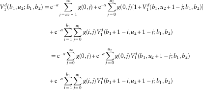
2. For u 1=b 1; u 2=0,1,…,b 2 −1, line 1’s premium income of 1 will be paid out as dividend if there is no claim for this line. Both lines will survive at time 1 if the claims X 1,1 and X 2,1 are no larger than b 1 – 1 and u 2, respectively, resulting in potential future dividends. This leads to
and $$\eqalignno{ V_{1}^{d} (b_{1} ,u_{2} ;b_{1} ,b_{2} )= & \,{\rm e}^{{{\minus}\alpha }} \mathop{\sum}\limits_{j\,=\,u_{2} \,{\plus}\,1}^\infty g(0,j){\plus}{\rm e}^{{{\minus}\alpha }} \mathop{\sum}\limits_{j\,=\,0}^{u_{2} } g(0,j)[1{\plus}V_{1}^{d} (b_{1} ,u_{2} {\plus}1\,{\minus}\,j;b_{1} ,b_{2} )] \cr & {\plus}{\rm e}^{{{\minus}\alpha }} \mathop{\sum}\limits_{i\,=\,1}^{b_{1} } \mathop{\sum}\limits_{j\,=\,0}^{u_{2} } g(i,j)V_{1}^{d} (b_{1} {\plus}1\,{\minus}\,i,u_{2} {\plus}1\,{\minus}\,j;b_{1} ,b_{2} ) \cr & = {\rm e}^{{{\minus}\alpha }} \mathop{\sum}\limits_{j\,=\,0}^\infty g(0,j){\plus}{\rm e}^{{{\minus}\alpha }} \mathop{\sum}\limits_{j\,=\,0}^{u_{2} } g(0,j)V_{1}^{d} (b_{1} ,u_{2} {\plus}1\,{\minus}\,j;b_{1} ,b_{2} ) \cr & {\plus}{\rm e}^{{{\minus}\alpha }} \mathop{\sum}\limits_{i\,=\,1}^{b_{1} } \mathop{\sum}\limits_{j\,=\,0}^{u_{2} } g(i,j)V_{1}^{d} (b_{1} {\plus}1\,{\minus}\,i,u_{2} {\plus}1\,{\minus}\,j;b_{1} ,b_{2} ) $$
 $$\eqalignno{ V_{2}^{d} (b_{1} ,u_{2} ;b_{1} ,b_{2} )= & \,{\rm e}^{{{\minus}\alpha }} \mathop{\sum}\limits_{j\,=\,0}^{u_{2} } g(0,j)V_{2}^{d} (b_{1} ,u_{2} {\plus}1\,{\minus}\,j;b_{1} ,b_{2} ) \cr & {\plus}{\rm e}^{{{\minus}\alpha }} \mathop{\sum}\limits_{i\,=\,1}^{b_{1} } \mathop{\sum}\limits_{j\,=\,0}^{u_{2} } g(i,j)V_{2}^{d} (b_{1} {\plus}1\,{\minus}\,i,u_{2} {\plus}1\,{\minus}\,j;b_{1} ,b_{2} ) $$
3. For u 1=0,1,…, b 1−1;u 2=b 2, the analyses are identical to those in Case 2 except that the roles of line 1 and line 2 are reversed. Hence, we have
and $$\eqalignno{ V_{1}^{d} (u_{1} ,b_{2} ;b_{1} ,b_{2} )= & \,{\rm e}^{{{\minus}\alpha }} \mathop{\sum}\limits_{i\,=\,0}^{u_{1} } g(i,0)V_{1}^{d} (u_{1} {\plus}1\,{\minus}\,i,b_{2} ;b_{1} ,b_{2} ) \cr & {\plus}{\rm e}^{{{\minus}\alpha }} \mathop{\sum}\limits_{i\,=\,0}^{u_{1} } \mathop{\sum}\limits_{j\,=\,1}^{b_{2} } g(i,j)V_{1}^{d} (u_{1} {\plus}1\,{\minus}\,i,b_{2} {\plus}1\,{\minus}\,j;b_{1} ,b_{2} ) $$
 $$\eqalignno{ V_{2}^{d} (u_{1} ,b_{2} ;b_{1} ,b_{2} )=\, & {\rm e}^{{{\minus}\alpha }} \mathop{\sum}\limits_{i\,=\,0}^\infty g(i,0){\plus}{\rm e}^{{{\minus}\alpha }} \mathop{\sum}\limits_{i=0}^{u_{1} } g(i,0)V_{2}^{d} (u_{1} {\plus}1\,{\minus}\,i,b_{2} ;b_{1} ,b_{2} ) \cr & {\plus}{\rm e}^{{{\minus}\alpha }} \mathop{\sum}\limits_{i\,=\,0}^{u_{1} } \mathop{\sum}\limits_{j\,=\,1}^{b_{2} } g(i,j)V_{2}^{d} (u_{1} {\plus}1\,{\minus}\,i,b_{2} {\plus}1\,{\minus}\,j;b_{1} ,b_{2} ) $$
4. For u 1=b 1; u 2=b 2, each line will pay out the premium income of 1 as dividend if it has no claim, plus potential future dividends if both lines survive time 1. This results in
and $$\eqalignno{ V_{1}^{d} (b_{1} ,b_{2} ;b_{1} ,b_{2} )= & \,{\rm e}^{{{\minus}\alpha }} g(0,0)V_{1}^{d} (b_{1} ,b_{2} ;b_{1} ,b_{2} ){\plus}{\rm e}^{{{\minus}\alpha }} \mathop{\sum}\limits_{j\,=\,0}^\infty g(0,j) \cr & {\plus}{\rm e}^{{{\minus}\alpha }} \mathop{\sum}\limits_{j\,=\,1}^{b_{2} } g(0,j)V_{1}^{d} (b_{1} ,b_{2} {\plus}1\,{\minus}\,j;b_{1} ,b_{2} ){\plus}{\rm e}^{{{\minus}\alpha }} \mathop{\sum}\limits_{i\,=\,1}^{b_{1} } g(i,0)V_{1}^{d} (b_{1} {\plus}1\,{\minus}\,i,b_{2} ;b_{1} ,b_{2} ) \cr & {\plus}{\rm e}^{{{\minus}\alpha }} \mathop{\sum}\limits_{i\,=\,1}^{b_{1} } \mathop{\sum}\limits_{j\,=\,1}^{b_{2} } g(i,j)V_{1}^{d} (b_{1} {\plus}1\,{\minus}\,i,b_{2} {\plus}1\,{\minus}\,j;b_{1} ,b_{2} ) $$
 $$\eqalignno{ V_{2}^{d} (b_{1} ,b_{2} ;b_{1} ,b_{2} )= & \,{\rm e}^{{{\minus}\alpha }} g(0,0)V_{2}^{d} (b_{1} ,b_{2} ;b_{1} ,b_{2} ){\plus}{\rm e}^{{{\minus}\alpha }} \mathop{\sum}\limits_{i\,=\,0}^\infty g(i,0) \cr & {\plus}{\rm e}^{{{\minus}\alpha }} \mathop{\sum}\limits_{j\,=\,1}^{b_{2} } g(0,j)V_{2}^{d} (b_{1} ,b_{2} {\plus}1\,{\minus}\,j;b_{1} ,b_{2} ){\plus}{\rm e}^{{{\minus}\alpha }} \mathop{\sum}\limits_{i\,=\,1}^{b_{1} } g(i,0)V_{2}^{d} (b_{1} {\plus}1\,{\minus}\,i,b_{2} ;b_{1} ,b_{2} ) \cr & {\plus}{\rm e}^{{{\minus}\alpha }} \mathop{\sum}\limits_{i\,=\,1}^{b_{1} } \mathop{\sum}\limits_{j\,=\,1}^{b_{2} } g(i,j)V_{2}^{d} (b_{1} {\plus}1\,{\minus}\,i,b_{2} {\plus}1\,{\minus}\,j;b_{1} ,b_{2} ) $$
To conclude, for fixed b 1 and b 2, the b 1b 2 equations of (5) at k=1, b 2 equations of (6), b 1 equations of (8) and the single equation (10) form a system of (b 1+1)(b 2+1) linear equations for {V 1d(u 1, u 2; b 1, b 2) : u 1=0,1,…,b 1; u 2=0,1,…,b 2} to be solved. Similarly, {V 2d(u 1, u 2; b 1, b 2) : u 1=0,1,…,b 1; u 2=0,1,…,b 2} can be solved from equation (5) at k=2 and equations (7), (9) and (11).
2.2. Deriving the approximation
Our goal is to approximate the expected discounted dividends V k defined in equation (2) for the continuous-time model (equation (1)) using the quantity V kd defined in equation (4) for the discrete-time model (equation (3)). To this end, we follow similar steps to those in Dickson & Waters (Reference Dickson and Waters1991), who studied the finite-time survival probabilities. Their approximation also proved to be useful in studying dividend problems as well (see Dickson & Waters, Reference Dickson and Waters2004; Cheung & Drekic, Reference Cheung and Drekic2008). However, the above applications were all conducted under univariate risk processes. Under the present bivariate framework, there are additional complications concerning the use of copula as well as a bivariate Panjer’s recursion (see section 2.3). The derivation of the approximation consists of the following four steps.
1. Step 1: Change of monetary unit
First, we apply a change of monetary unit in the continuous-time model (equation (1)). In particular, for some positive constants β 1 and β 2 (known as scaling factors), define the random variables Y k(1)=β kY k and Z k(1)=β kZ k for k=1, 2. If V k(1)(u 1, u 2; b 1, b 2) denotes the expected discounted dividends for line k in the continuous-time model with generic jumps Y 1(1), Y 2(1) and (Z 1(1), Z 2(1)), Poisson rates λ 11, λ 22 and λ 12, force of interest δ, premium rates (β 1c 1, β 2c 2), initial surplus levels (u 1, u 2) and barrier levels (b 1, b 2), it is immediate that V k in equation (2) satisfies
 $$V_{k} (u_{1} ,u_{2} ;b_{1} ,b_{2} )={1 \over {\beta _{k} }}V_{k}^{{(1)}} (\beta _{1} u_{1} ,\beta _{2} u_{2} ;\beta _{1} b_{1} ,\beta _{2} b_{2} )$$
Note that the copula for the scaled version (Z 1(1), Z 2(1)) is also C(⋅,⋅), i.e., identical to that of (Z 1, Z 2) (see e.g. Denuit et al. Reference Denuit, Dhaene, Goovaerts and Kaas2005, Proposition 4.4.4(i)).
2. Step 2: Discretisation of Y 1(1), Y 2(1), Z 1(1)and Z 2(1)
The random variables Y 1(1), Y 2(1), Z 1(1) and Z 2(1) defined in Step 1 are then discretised on {0,1, …} to give the discretised versions Y 1(2), Y 2(2), Z 1(2) and Z 2(2). The “mean preserving method” (see e.g. De Vylder & Goovaerts, Reference De Vylder and Goovaerts1988, section 7; Dickson, Reference Dickson2005: 80) is suggested and it is known to yield good results (see Dickson & Waters, Reference Dickson and Waters1991, Reference Dickson and Waters2004; Cheung & Drekic, Reference Cheung and Drekic2008). The pmf of Y k(2) is given by, for k=1, 2:
 $$h_{{kk}} (i)=\beta _{k} \left( {\mathop{\int}\nolimits_{{i \over {\beta _{k} }}}^{{{i\,{\plus}\,1} \over {\beta _{k} }}} F_{{kk}} (y)\:dy\,{\minus}\,\mathop{\int}\nolimits_{{{i{\minus}1} \over {\beta _{k} }}}^{{i \over {\beta _{k} }}} F_{{kk}} (y)\:dy} \right),\quad \quad i=0,1,\,\ldots\,$$
For the discretised random vector (Z 1(2), Z 2(2)), we apply the same copula C(⋅,⋅) as the dependency structure (see e.g. Bargès et al., Reference Bargès, Cossette and Marceau2009, section 5.2). Therefore, the joint pmf of (Z 1(2), Z 2(2)), namely h 12(i, j), can be calculated from the associated joint cdf:
 $$\mathop{\sum}\limits_{k\,=\,0}^i \mathop{\sum}\limits_{l\,=\,0}^j h_{{12}} (k,l)=C\left( {\beta _{1} \mathop{\int}\nolimits_{{i \over {\beta _{1} }}}^{{{i\,{\plus}\,1} \over {\beta _{1} }}} F_{{1{\bullet}}} (y)\:dy,\beta _{2} \mathop{\int}\nolimits_{{j \over {\beta _{2} }}}^{{{j\,{\plus}\,1} \over {\beta _{2} }}} F_{{{\bullet}2}} (y)\:dy} \right),\quad \quad i,j=0,1,\,\ldots\,$$
Denote by V k(2)(u 1, u 2; b 1, b 2) the expected discounted dividends for line k in the continuous-time model with discrete generic jumps Y 1(2), Y 2(2) and (Z 1(2), Z 2(2)), Poisson rates λ 11, λ 22 and λ 12, force of interest δ, premium rates (β 1c 1, β 2c 2), initial surplus levels (u 1, u 2) and barrier levels (b 1, b 2). If Y 1(2), Y 2(2) and (Z 1(2), Z 2(2)) are good approximations of Y 1(1), Y 2(1) and (Z 1(1), Z 2(1)) (i.e. when β 1 and β 2 are “large”), respectively, then
and hence from equation (12) one has $$V_{k}^{{(2)}} (u_{1} ,u_{2} ;b_{1} ,b_{2} )\,\simeq\,V_{k}^{{(1)}} (u_{1} ,u_{2} ;b_{1} ,b_{2} )$$
 $$V_{k} (u_{1} ,u_{2} ;b_{1} ,b_{2} )\,\simeq\,{1 \over {\beta _{k} }}V_{k}^{{(2)}} (\beta _{1} u_{1} ,\beta _{2} u_{2} ;\beta _{1} b_{1} ,\beta _{2} b_{2} )$$
3. Step 3: Change of time unit
We now change the time unit of the continuous-time model with discrete claims in Step 2 such that the premium income per time unit is 1. To achieve this, β 1 and β 2 introduced in Step 1 are chosen such that β 1c 1=β 2c 2. The model in Step 2 is then equivalent to a model in which the discrete generic jumps are Y 1(2), Y 2(2) and (Z 1(2), Z 2(2)), the Poisson rates are λ 11/β 1c 1, λ 22/β 1c 1 and λ 12/β 1c 1, the force of interest is α=δ/β 1c 1, the premium rates are (1, 1), the initial surplus levels are (u 1, u 2) and the barrier levels are (b 1, b 2). If we denote by V k(3)(u 1, u 2; b 1, b 2) the expected discounted dividends for line k under the above setting, then
and hence from equation (15) we arrive at $$V_{k}^{{(3)}} (u_{1} ,u_{2} ;b_{1} ,b_{2} )=V_{k}^{{(2)}} (u_{1} ,u_{2} ;b_{1} ,b_{2} )$$
 $$V_{k} (u_{1} ,u_{2} ;b_{1} ,b_{2} )\,\simeq\,{1 \over {\beta _{k} }}V_{k}^{{(3)}} (\beta _{1} u_{1} ,\beta _{2} u_{2} ;\beta _{1} b_{1} ,\beta _{2} b_{2} )$$
4. Step 4: Replacement of continuous-time model by discrete-time model
In this final step, the continuous-time model with discrete claims in Step 3 is replaced by a discrete-time one (in which the event of ruin and the payment of dividend (if any) are only monitored once per period). One can then approximate V k(3)(u 1, u 2; b 1, b 2) by
where V kd(u 1, u 2; b 1, b 2) is defined by equation (4) under the force of interest α=δ/β 1c 1 and the generic discrete claims, for k=1, 2: $$V_{k}^{{(3)}} (u_{1} ,u_{2} ;b_{1} ,b_{2} )\,\simeq\,V_{k}^{d} (u_{1} ,u_{2} ;b_{1} ,b_{2} )$$
 $$X_{k} =\mathop{\sum}\limits_{n\,=\,1}^{M_{{kk}} } Y_{{k,n}}^{{(2)}} {\plus}\mathop{\sum}\limits_{n\,=\,1}^{M_{{12}} } Z_{{k,n}}^{{(2)}} $$
In the above representation, M kk has a Poisson distribution with mean γ kk=λ kk/β 1c 1 whereas M 12 has a Poisson distribution with mean γ 12=λ 12/β 1c 1. Moreover,
 $$\{ Y_{{k,n}}^{{(2)}} \} _{{n\,=\,1}}^{\infty} $$
is i.i.d. with generic variable Y k(2), and
  $$\{ (Z_{{1,n}}^{{(2)}} ,Z_{{2,n}}^{{(2)}} )\} _{{n\,=\,1}}^{\infty} $$
is also i.i.d. with generic vector (Z 1(2),Z 2(2)). In addition, M 11, M 22, M 12,
  $$\{ Y_{{1,n}}^{{(2)}} \} _{{n\,=\,1}}^{\infty} ,\,\,\{ Y_{{2,n}}^{{(2)}} \} _{{n\,=\,1}}^{\infty} \;{\rm and}\;\{ (Z_{{1,n}}^{{(2)}} ,Z_{{2,n}}^{{(2)}} )\} _{{n\,=\,1}}^{\infty} $$
are all mutually independent. Hence X 1 and X 2 are dependent compound Poisson random variables. When β 1 (and hence β 2) is “large”, the time intervals between the points where the surplus levels are checked are small, since one time unit in the present step is equivalent to 1/β 1c 1 time unit in the original continuous-time model (equation (1)). Then equation (17) will be a good approximation. To conclude, one has from equation (16) that
 $$V_{k} (u_{1} ,u_{2} ;b_{1} ,b_{2} )\,\simeq\,{1 \over {\beta _{k} }}V_{k}^{d} (\beta _{1} u_{1} ,\beta _{2} u_{2} ;\beta _{1} b_{1} ,\beta _{2} b_{2} )$$
and one requires β 1u 1, β 2u 2, β 1b 1 and β 2b 2 to be integers.
Formula (19) suggests that its left-hand side, namely the expected discounted dividends V k in equation (2) for the continuous-time model (equation (1)), can be approximated by its right-hand side that is in terms of V kd defined in equation (4) for the fully discrete model (equation (3)). It remains to evaluate the joint pmf of (X 1, X 2), namely g(i, j), in order to apply the results in section 2.1 to find V kd. This will be the subject matter of the next subsection via the use of Panjer-type recursion (see e.g. Klugman et al., Reference Klugman, Panjer and Willmot2008, Chapter 6.8). Note also that the above approximation is different from that in Yuen et al. (Reference Yuen, Guo and Wu2006, section 3), who approximated a bivariate compound Poisson risk model by a bivariate compound binomial model. Their approximation does not involve Panjer’s recursion for compound distribution, and in their model a common shock does not result in dependent claims in the two lines.
2.3. Bivariate Panjer's recursion for dependent compound Poisson distributions
With the components of the random vector (X 1, X 2) given by equation (18), the derivation of its joint pmf g(i, j) can be done by slightly modifying the results in Walhin & Paris (Reference Walhin and Paris2000, section 4) who considered the case where Z 1(2) and Z 2(2) are independent and distributed as Y 1(2) and Y 2(2), respectively. Under the current setting, defining the probability generating function ![]() $$\hat{g}(r,s)=\mathop{\sum}\nolimits_{i\,=\,0}^\infty \mathop{\sum}\nolimits_{j\,=\,0}^\infty r^{i} s^{j} g(i,j)$$
, it can be proved that
$$\hat{g}(r,s)=\mathop{\sum}\nolimits_{i\,=\,0}^\infty \mathop{\sum}\nolimits_{j\,=\,0}^\infty r^{i} s^{j} g(i,j)$$
, it can be proved that
where ![]() $$\hat{h}_{{11}} (r)=\mathop{\sum}\nolimits_{i\,=\,0}^\infty r^{i} h_{{11}} (i)$$
,
$$\hat{h}_{{11}} (r)=\mathop{\sum}\nolimits_{i\,=\,0}^\infty r^{i} h_{{11}} (i)$$
, ![]() $$\hat{h}_{{22}} (s)=\mathop{\sum}\nolimits_{j\,=\,0}^\infty s^{j} h_{{22}} (j)$$
and
$$\hat{h}_{{22}} (s)=\mathop{\sum}\nolimits_{j\,=\,0}^\infty s^{j} h_{{22}} (j)$$
and ![]() $$\hat{h}_{{12}} (r,s)=\mathop{\sum}\nolimits_{i\,=\,0}^\infty \mathop{\sum}\nolimits_{j\,=\,0}^\infty r^{i} s^{j} h_{{12}} (i,j)$$
are the probability generating functions pertaining to the pmf’s h 11(⋅), h 22(⋅) and h 12(⋅,⋅) defined via equations (13) and (14) in Step 2; whereas γ 11=λ 11/β 1c 1, γ 22=λ 22/β 1c 1 and γ 12=λ 12/β 1c 1 according to Step 4. By differentiating the above equation with respect to r, multiplying the resulting equation by r and then equating coefficients of r i, we arrive at
$$\hat{h}_{{12}} (r,s)=\mathop{\sum}\nolimits_{i\,=\,0}^\infty \mathop{\sum}\nolimits_{j\,=\,0}^\infty r^{i} s^{j} h_{{12}} (i,j)$$
are the probability generating functions pertaining to the pmf’s h 11(⋅), h 22(⋅) and h 12(⋅,⋅) defined via equations (13) and (14) in Step 2; whereas γ 11=λ 11/β 1c 1, γ 22=λ 22/β 1c 1 and γ 12=λ 12/β 1c 1 according to Step 4. By differentiating the above equation with respect to r, multiplying the resulting equation by r and then equating coefficients of r i, we arrive at
 $$\eqalignno{ & g(i,j)=\gamma _{{11}} \mathop{\sum}\limits_{k=1}^i {k \over i}h_{{11}} (k)g(i\,{\minus}\,k,j){\plus}\gamma _{{12}} \mathop{\sum}\limits_{k=1}^i \mathop{\sum}\limits_{l=0}^j {k \over i}h_{{12}} (k,l)g(i\,{\minus}\,k,j\,{\minus}\,l), \cr & \quad \quad i=1,2,\,\ldots\,;j=0,1,\,\ldots\, $$
Similarly,
 $$\eqalignno{ & g(i,j)=\gamma _{{22}} \mathop{\sum}\limits_{l\,=\,1}^j {l \over j}h_{{22}} (l)g(i,j\,{\minus}\,l){\plus}\gamma _{{12}} \mathop{\sum}\limits_{k\,=\,0}^i \mathop{\sum}\limits_{l\,=\,1}^j {l \over j}h_{{12}} (k,l)g(i\,{\minus}\,k,j\,{\minus}\,l), \cr & \quad \quad i=0,1,\,\ldots\,;j=1,2,\,\ldots\, $$
The starting point of the recursion is
2.4. Numerical illustrations of the approximation
This subsection aims at demonstrating the quality of the approximation derived in section 2.2. Since the same approximation will be used in various numerical illustrations for the rest of the paper, we highlight the procedures as far as programming work is concerned to approximate V k(u 1, u 2; b 1, b 2) for k=1, 2.
∙ Specify the parameters and distributional assumptions of the continuous-time model (equation (1)), which include the premium rates (c 1, c 2), the Poisson rates (λ 11, λ 22, λ 12), the cdfs F 11(⋅), F 22(⋅) and F 12(⋅,⋅), and the copula C(⋅,⋅). Specify the force of interest δ for the dividend function in equation (2).
∙ Select the scaling factors (β 1, β 2) such that β 1u 1, β 2u 2, β 1b 1 and β 2b 2 are integers, and β 1c 1=β 2c 2.
∙ Apply equations (13) and (14) to find h 11(⋅), h 22(⋅) and h 12(⋅,⋅).
∙ With γ 11=λ 11/β 1c 1, γ 22=λ 22/β 1c 1 and γ 12=λ 12/β 1c 1, evaluate g(⋅,⋅) recursively using equations (20) and (21) subject to the starting point in equation (22).
∙ Set α=δ/β 1c 1. Apply equations (5)–(11) (with b 1 and b 2 replaced by β 1b 1 and β 2b 2, respectively) to calculate {V 1d(u 1, u 2; β 1b 1, β 2b 2): u 1=0,1,…, β 1b 1; u 2=0,1,…, β 2b 2} and {V 2d(u 1, u 2; β 1b 1, β 2b 2) : u 1=0,1,…, β 1b 1; u 2=0,1,…, β 2b 2}.
∙ Apply equation (19) to approximate V k(u 1, u 2; b 1, b 2) for k=1, 2.
It is instructive to note that as the scaling factors β 1 and β 2 increase (such that β 1c 1=β 2c 2), the approximation of the continuous-time bivariate process by a discrete-time one gets more accurate because (i) the discretisation in Step 2 in section 2.2 gets finer (i.e. continuous claims are better approximated by discrete ones); and (ii) the approximating discrete-time process in Step 4 is checked more frequently (and becomes closer to the continuous-time model). Note that two opposing sources of errors always occur when one approximates the dividend function V k by V kd. First, dividends are paid immediately in the continuous-time model once the surplus of an individual line reaches its barrier; whereas in the discrete-time model, reaching the barrier does not immediately result in a dividend unless there is no claim in the next period. In this aspect, V kd tends to underestimate the true value V k due to discounting. In contrast, the discrete-time model tends to survive longer due to the protection from delayed dividend payments, which means that there can be more potential future dividends. This may cause V kd to overestimate V k. In the following example, we shall gradually increase the scaling factors in computing the approximated dividend values. Simulations are also conducted to verify the accuracy of the approximations and check whether one of the aforementioned effects is always more dominant.
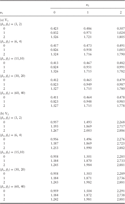
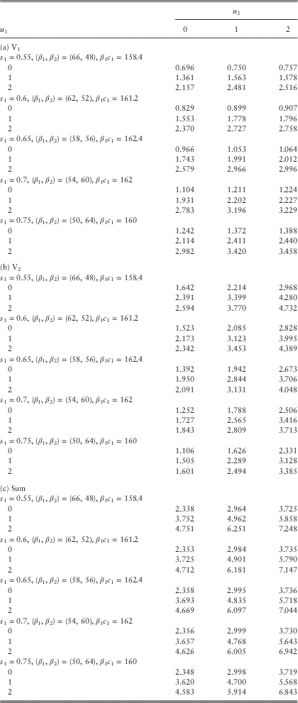
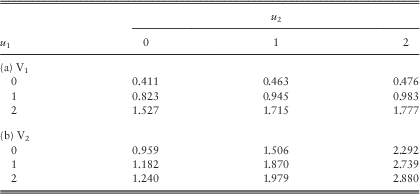
Example 1 In this example, we assume the Poisson rates λ 11=λ 22=λ 12=1 and the premium rates c 1=2.8 and c 2=4.2. Line 1 is subject to claims with pdf f 11(y)=f 1∙(y)=0.8e−0.8y; whereas the claims of line 2 have pdf f 22(y)=f ∙2(y)=0.5e−0.5y. Their means are 1.25 and 2, respectively, and they both have coefficient of variation of 1. In the case of a common shock, it is assumed that Z 1 and Z 2 are independent of each other, i.e., the independence copula C(u,v)=uv for 0≤u, v≤1 is used. The loading conditions c 1=2.8>2.5=λ 11E[Y 1]+λ 12E[Z 1] and c 2=4.2>4=λ 22E[Y 2]+λ 12E[Z 2] are satisfied. The force of interest is assumed to be δ=0.05, and the barrier values are fixed to be b 1=b 2=2 (see section 5 for an explanation regarding the choice of low barriers). According to the computational procedures outlined at the beginning of this subsection, we require β 1c 1=β 2c 2, or equivalently β 1=1.5β 2. The approximated values of the expected discounted dividends for the two lines using different sets of (β 1, β 2) are given in Tables 1a and 1b.
Table 1 Approximated dividends in the two lines for various sets (β 1, β 2): (a) V1 and (b) V2.

From Table 1, it is clear that for a given set of (β 1, β 2), the dividend functions for both lines are increasing in the initial surplus levels u 1 and u 2 as they must be. When we increase the values of (β 1, β 2) for each fixed pair of initial surplus levels (u 1, u 2), the dividend values of line 1 always decrease (except when (u 1, u 2)=(2, 0)); whereas those of line 2 either increase or decrease. In all cases, the dividends for both lines appear to be converging as (β 1, β 2) increases. To further verify the results, we have also run some simulations in the continuous-time risk model and obtained Tables 2a and 2b for the dividend functions of the two lines. In Table 2, each pair of (V 1, V 2) is calculated using 1,000,000 sample paths generated up to the joint ruin time. Comparing Table 1 with Table 2, it can be seen that scaling factors of (β 1, β 2)=(60, 40) produce very good results: the dividend values are always the same up to at least two decimal places. More interestingly, the results obtained by smaller scaling factors of, say (β 1, β 2)=(15, 10), are indeed still comparable to those by simulations. However, the simulation results are sometimes a bit larger than and sometimes a bit smaller than the discrete-time approximations. Therefore, one cannot conclude whether our approximation tends to underestimate or overestimate the true value of dividends, i.e., neither the effect of delayed dividends nor the effect of prolonged survival is always more dominant. Nonetheless, for each fixed pair of initial surplus levels (u 1, u 2), the approximated values in Table 1 approach the corresponding simulated values in Table 2 either from above or below as (β 1, β 2) increase. (Indeed, we have separately run the Dickson−Waters type of algorithm in Cheung & Drekic, Reference Cheung and Drekic2008 for a single line dual risk process with a dividend barrier. It was found that the approximated dividend values either increase or decrease to the true value as the scaling factor increases, depending on the initial surplus and the barrier level). □
Table 2 Simulated dividends in the two lines: (a) V1 and (b) V2.
3. Three Different Types of Dependencies
In this section, we examine the bivariate risk process described by equation (1) in which the two lines of business are subject to different types of dependencies via some numerical examples. These include (i) common shocks; (ii) copulas; and (iii) proportional reinsurance. Throughout this entire section, the barrier values b 1=b 2=2 are applied because high scaling factors (β 1, β 2) will be used (see concluding remarks in section 5).
3.1. Different levels of common shocks
Example 2 In this example, we aim at examining the impact of different levels of common shocks on the dividends by varying the values of λ 11, λ 22 and λ 12 while keeping λ 11+λ 12=λ 22+λ 12=2 fixed, i.e., each individual line of business is subject to the same total claim arrival rate of 2. To illustrate the versatility of the approximation, we use the more complicated density functions ![]() $$f_{{11}} (y)=f_{{1{\bullet}}} (y)=8{\rm e}^{{{\minus}2y}} {\rm sin}^2 y$$
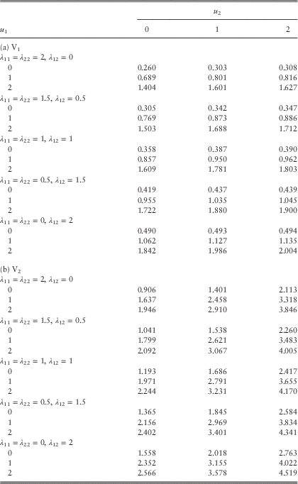
, f 22(y)=f ∙2(y)=(1/4)(0.62ye−0.6y)+(3/4)(92ye−9y). These two distributions have rational Laplace transforms, and they were used in Cheung & Drekic (Reference Cheung and Drekic2008). They both have mean 1, and their coefficients of variation are 0.50 and 1.80, respectively. While f 22(y) represents a standard mixture of two Erlang (2) distributions, the less common f 11(y) is the pdf of a damped squared sine distribution with low variability. In particular, the density f 11(y) is strictly increasing starting from f 11(0)=0 until it reaches the global maximum of 0.83152 at π/4=0.78540, from which f 11(y) is strictly decreasing until zero is reached at π=3.14159. Due to the periodicity induced by the sine function, f 11(y) also achieves (i) global and local minimum of zero at y=nπ for n=1,2,…; and (ii) local maximum at y=nπ+π/4 for n=1,2,…. Nonetheless, f 11(y) is very very close to zero for y>π, and f 11(y) is strictly unimodal for y≥0. The premium rates are assumed to be c 1=2.2 and c 2=3.3, so that the loading conditions c 1=2.2>2=λ 11E[Y 1]+λ 12E[Z 1] and c 2=3.3>2=λ 22E[Y 2]+λ 12E[Z 2] hold true. (Note that the premium of line 2 is assumed to have a larger loading factor because its claims have larger variance.) The remaining model assumptions are same as those in Example 1: Z 1 and Z 2 are independent in case of a common shock; the force of interest is δ=0.05, and the barrier values are b 1=b 2=2. Using the scaling factors (β 1, β 2)=(60, 40), we follow the approximation procedures outlined at the beginning of section 2.4 and the resulting dividend values are listed in Tables 3a and 3b. The tables start with the extreme case of λ 11=λ 22=2 and λ 12=0 in which the two lines of business only face their own claims independently with no common shocks at all. Then as we move down the tables, λ 11 and λ 22 are decreased by 0.5 whereas λ 12 is increased by 0.5 each time until we reach another extreme case where λ 11=λ 22=0 and λ 12=2. The last case indicates that the two lines are only subject to common shocks.
$$f_{{11}} (y)=f_{{1{\bullet}}} (y)=8{\rm e}^{{{\minus}2y}} {\rm sin}^2 y$$
, f 22(y)=f ∙2(y)=(1/4)(0.62ye−0.6y)+(3/4)(92ye−9y). These two distributions have rational Laplace transforms, and they were used in Cheung & Drekic (Reference Cheung and Drekic2008). They both have mean 1, and their coefficients of variation are 0.50 and 1.80, respectively. While f 22(y) represents a standard mixture of two Erlang (2) distributions, the less common f 11(y) is the pdf of a damped squared sine distribution with low variability. In particular, the density f 11(y) is strictly increasing starting from f 11(0)=0 until it reaches the global maximum of 0.83152 at π/4=0.78540, from which f 11(y) is strictly decreasing until zero is reached at π=3.14159. Due to the periodicity induced by the sine function, f 11(y) also achieves (i) global and local minimum of zero at y=nπ for n=1,2,…; and (ii) local maximum at y=nπ+π/4 for n=1,2,…. Nonetheless, f 11(y) is very very close to zero for y>π, and f 11(y) is strictly unimodal for y≥0. The premium rates are assumed to be c 1=2.2 and c 2=3.3, so that the loading conditions c 1=2.2>2=λ 11E[Y 1]+λ 12E[Z 1] and c 2=3.3>2=λ 22E[Y 2]+λ 12E[Z 2] hold true. (Note that the premium of line 2 is assumed to have a larger loading factor because its claims have larger variance.) The remaining model assumptions are same as those in Example 1: Z 1 and Z 2 are independent in case of a common shock; the force of interest is δ=0.05, and the barrier values are b 1=b 2=2. Using the scaling factors (β 1, β 2)=(60, 40), we follow the approximation procedures outlined at the beginning of section 2.4 and the resulting dividend values are listed in Tables 3a and 3b. The tables start with the extreme case of λ 11=λ 22=2 and λ 12=0 in which the two lines of business only face their own claims independently with no common shocks at all. Then as we move down the tables, λ 11 and λ 22 are decreased by 0.5 whereas λ 12 is increased by 0.5 each time until we reach another extreme case where λ 11=λ 22=0 and λ 12=2. The last case indicates that the two lines are only subject to common shocks.
Table 3 Approximated dividends in the two lines for different levels of common shocks: (a) V1 and (b) V2.

A look at Table 3 reveals that the dividend values for both lines increase as the rate of common shocks increases. This can be interpreted as follows. For the case where λ 11=λ 22=2 and λ 12=0, the surplus processes of the two lines are indeed independent, and the mean total number of claim events per unit time, namely λ 11+λ 22+λ 12, is 4. As we move towards the most dependent case of λ 11=λ 22=0 and λ 12=2 where there are common shocks only, the mean total number of claim events per unit time decreases to 2. Since each instant of a claim event can potentially be the joint ruin time T=min(T 1, T 2), the bivariate process is likely to survive longer when there are more common shocks (keeping the total claim arrival rate for each line fixed), resulting in more dividends. Note that the dividends for both lines cease once ruin has occurred in one of the two lines. Another interpretation of our results is that when there are no common shocks at all, one of the lines in fact has positive surplus at the joint ruin time T but no further dividends are paid, i.e., the situation is not economical. In contrast, when common shocks are more frequent, it is more likely that both lines have negative surplus at the joint ruin time T anyway, i.e., there is less chance that resources are wasted. These observations complement the numerical results in Gong et al. (Reference Gong, Badescu and Cheung2012, figure 1) who studied the joint ruin probability in the absence of dividends. □
3.2. Different copulas
In this subsection, we apply different parametric copulas to describe the dependency between Z 1 and Z 2 when a common shock strikes both lines. Three copulas will be considered: (i) Ali−Mikhail−Haq (AMH) copula (e.g. Nelsen, Reference Nelsen2006, Exercises 2.14(d) and 5.10); (ii) Farlie−Gumbel−Morgenstern (FGM) copula (e.g. Nelsen, Reference Nelsen2006, Examples 3.12 and 5.2); and (iii) Gaussian (or normal) copula (e.g. Denuit et al., Reference Denuit, Dhaene, Goovaerts and Kaas2005, Chapter 4.3.3 and Exercise 5.4.6). Each copula’s definition and Kendall’s τ (or Kendall’s rank correlation coefficient) are summarised in Table 4.
Table 4 Copulas and their Kendall’s rank correlation coefficients.

In the definition of the Gaussian copula, Φ(⋅) is the standard normal cdf whereas Φθ(⋅,⋅) represents the bivariate standard normal cdf with covariance θ. Note that the Kendall’s rank correlation coefficient, as a measure of dependency, is only specific to a given copula and is independent of the marginal distributions (e.g. Nelsen, Reference Nelsen2006, Theorem 5.1.3). In all three copulas, θ=0 corresponds to the case of independence (i.e. C(u, v)=uv for 0≤u, v≤1), and the resulting Kendall’s τ is zero. It is instructive to note that all these three copulas have one parameter. This means that from the point of view of calibration, if one of these copulas has been identified as suitable for a given set of data, then the parameter follows in a straightforward manner once the Kendall’s rank correlation has been estimated (see e.g. McNeil et al., Reference McNeil, Frey and Embrechts2005, section 5.5.1).
The application of copulas as a tool for risk management in finance and insurance was discussed extensively in Embrechts et al. (Reference Embrechts, McNeil and Straumann2002, Reference Embrechts, Lindskog and McNeil2003), and we also refer interested readers to Frees & Valdez (Reference Frees and Valdez1998), Klugman & Parsa (Reference Klugman and Parsa1999) and Trivedi & Zimmer (Reference Trivedi and Zimmer2005) for general actuarial applications and fitting of bivariate loss distributions using copulas. The reasons for the choice of the above three copulas are as follows. First, the AMH copula belongs to the class of Archimedean copulas, which possess nice properties and are popular for modelling (see e.g. Genest & MacKay, Reference Genest and MacKay1986; Denuit et al., Reference Denuit, Dhaene, Goovaerts and Kaas2005, Chapter 4.5; Nelsen, Reference Nelsen2006, Chapter 4). See also Denuit et al. (Reference Denuit, Purcaru and Van Keilegom2004) for the use of Archimedean copulas in non-life insurance. A plot of the AMH copula pdf can be found in Panjer (Reference Panjer2006, figure 8.8). Second, the FGM copula belongs to the class of polynomial copulas (see e.g. Drouet-Mari & Kotz, Reference Drouet-Mari and Kotz2001, Chapter 4.5.2). It is a tractable copula that is a first-order approximation of both the Plackett copula and the Frank copula (see e.g. Nelsen, Reference Nelsen2006, Exercises 3.39 and 4.9). Owing to its simplicity, the FGM copula has become increasingly popular in modelling aggregate claims in insurance risk models (see e.g. Cossette et al., Reference Cossette, Marceau and Marri2010; Bargès et al., Reference Bargès, Cossette, Loisel and Marceau2011; Woo & Cheung, Reference Woo and Cheung2013, section 4; Chadjiconstantinidis & Vrontos, Reference Chadjiconstantinidis and Vrontos2014). While AMH and FGM copulas only allow moderate dependence (which is evident from the range of Kendall’s τ), stronger dependency can be modelled by the Gaussian copula that is commonly used for comparison purposes. See e.g. Denuit et al. (Reference Denuit, Dhaene, Goovaerts and Kaas2005, figure 4) that depicts the increasing dependency of the components of a bivariate Gaussian copula as θ increases. It is known (e.g. Trivedi & Zimmer, Reference Trivedi and Zimmer2005, Chapter 2.3.3) that the bivariate Gaussian copula attains the Fréchet lower and upper bounds, respectively, when θ tends to −1 and 1.
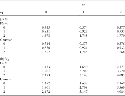
Example 3 In this example, we follow the same assumptions as in Example 2 of section 3.1 under the Poisson rates λ 11=λ 22=λ 12=1, except that the three copulas in Table 4 are applied to the pair (Z 1, Z 2) arising from common shocks. For a fair comparison among different copulas, we fix the value of Kendall’s τ and then solve for the appropriate parameter θ. First, setting τ=0.2 yields θ=0.71349, θ=0.9 and θ=0.30902, respectively, for AMH, FGM and Gaussian copulas. Tables 5a and 5b summarise the approximated dividend values calculated using the procedures at the beginning of section 2.4 under the scaling factors (β 1, β 2)=(60, 40). If we instead fix a negative Kendall’s τ=−0.2, it is found that θ=−0.9 and θ=−0.30902 for FGM and Gaussian copulas, respectively; whereas the AMH copula cannot reach such a Kendall’s τ according to the last column of Table 4. The corresponding approximated dividend values are given in Tables Reference Badescu, Cheung and Rabehasaina6a and 6b.
Table 5 Approximated dividends in the two lines for different copulas with τ=0.2: (a) V1 and (b) V2.
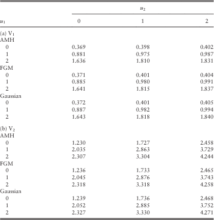
Table 6 Approximated dividends in the two lines for different copulas with τ=−0.2: (a) V1 and (b) V2.

Within each of the four Tables 5a & 5b and Reference Badescu, Cheung and Rabehasaina6a & 6b, it is clear that the dividend values are considerably close for different copulas with the Kendall’s τ being fixed. When one compares the values across Tables 3 (i.e. the case with λ 11=λ 22=λ 12=1), 5 and 6, the dividend function for each line increases as the Kendall’s τ changes from −0.2 to 0 and then to 0.2. The intuition behind is as follows. For each of the three copulas, for fixed (u, v) the value of C(u, v) increases with the parameter θ, which in turn increases with the Kendall’s τ. Thus, for fixed values of z 1 and z 2, the joint cdf F 12(z 1,z 2)=C(F 1∙(z 1), F ∙2(z 2)) increases with respect to the Kendall’s τ. In other words, when dependency is positive, the possibility for (Z 1, Z 2) to lie outside (0, z 1]×(0, z 2] is smaller, leading to less chance of ruin of the bivariate process from a given common shock and hence more dividends. □
3.3. Proportional reinsurance
In this subsection, we illustrate the interpretation and application of our model described by equation (1) in problems involving proportional reinsurance (see Remark 1). To begin, we first discuss the formulation and some notations that will be used throughout. In the absence of any reinsurance, it is assumed that line 1 of business faces two independent classes of aggregate claims with Poisson arrival rates λ 11 and λ 12 and generic claim severities Y 1 and W, respectively. In addition, line 2 is only subject to an aggregate claims process with Poisson rate λ 22 and generic claim Y 2. Suppose that the generic claim W is more dangerous than Y 1 (e.g. W is heavy-tail and Y 1 is light-tail), and line 1 wants to reduce its risk exposure by purchasing reinsurance from line 2 for part of the risk W. We assume a proportional reinsurance contract such that line 1 retains a proportion s 1 of each claim W (and reinsures the remaining portion of 1−s 1) for some 0<s 1<1. Under the reinsurance arrangements described above, the model in equation (1) is applicable by letting (Z 1, Z 2)=(s 1W,(1−s 1)W). With F W(⋅) being the cdf of the positive continuous random variable W, one has F 1∙(y 1)=F W(y 1/s 1) and F ∙2(y 2)=F W(y 2/(1−s 1)). Because Z 1 and Z 2 are comonotonic, the comonotonicity copula C(u, v)=min(u, v) for 0≤u, v≤1 should be applied. It is assumed that line 1 imposes the security loading factors η 11 and η 12 to the claims Y 1 and W; whereas line 2 imposes the loadings η 21 and η 22 to Y 2 and Z 2. Thus, the net premium income rates c 1 and c 2 are given by
Practically, the loading factor η 22 charged by the reinsurer is no less than the loading η 12. Otherwise, line 1 can simply reinsure the entire risk W to earn a risk-free profit. In addition, line 1 of business should not choose to accept the risk W unless it can generate positive expected net profit. This gives rise to the condition
The left-hand side of the above equation represents the net premium income of line 1 upon accepting the risk W and reinsuring part of it; while the right-hand side is line 1’s expected net claims arising from W after reinsurance.
Example 4 In this example, we assume λ 11=λ 22=λ 12=1, ![]() $$f_{{11}} (y)=8{\rm e}^{{{\minus}2y}} {\rm sin}^2 y$$
, f W(y)=5⋅85/(y+8)6 and f 22(y)=(1/4)(0.62ye−0.6y)+(3/4)(92ye−9y). Note that Y 1 and Y 2 are both light-tail with mean 1 while W is heavy-tail with mean 2. As in previous examples, the force of interest is assumed to be δ=0.05 and the barrier values are (b 1, b 2)=(2, 2). In addition, the loading factors are η 11=0.2, η 12=η 21=0.5 and η 22=1. Plugging in these assumptions into the inequality (equation (24)) yields s 1>0.5. Then, the values of c 1 and c 2 are calculated according to equation (23) based on different choices of s 1. We shall again apply the approximation procedures stated in section 2.4 to produce the dividend values. Note that it is not possible to apply the same scaling factors (β 1, β 2) for different values of s 1 due to the constraint β 1c 1=β 2c 2. In order to make a fair comparison of the dividends across different s 1, the values of β 1 (or β 2) are chosen such that the resulting values of β 1c 1 (or β 2c 2) are comparable for different s 1, so that the approximating discrete-time processes are checked at roughly the same frequency. (Recall that one time unit in the approximating discrete-time model is equivalent to 1/β 1c 1 time unit in the continuous-time model.) Our study is performed under a set of (β 1, β 2) whose values of β 1c 1 are all around 160. The approximated expected discounted dividends for the two lines as well as their sums for various values of s 1 are given in Tables 7a−7c.
$$f_{{11}} (y)=8{\rm e}^{{{\minus}2y}} {\rm sin}^2 y$$
, f W(y)=5⋅85/(y+8)6 and f 22(y)=(1/4)(0.62ye−0.6y)+(3/4)(92ye−9y). Note that Y 1 and Y 2 are both light-tail with mean 1 while W is heavy-tail with mean 2. As in previous examples, the force of interest is assumed to be δ=0.05 and the barrier values are (b 1, b 2)=(2, 2). In addition, the loading factors are η 11=0.2, η 12=η 21=0.5 and η 22=1. Plugging in these assumptions into the inequality (equation (24)) yields s 1>0.5. Then, the values of c 1 and c 2 are calculated according to equation (23) based on different choices of s 1. We shall again apply the approximation procedures stated in section 2.4 to produce the dividend values. Note that it is not possible to apply the same scaling factors (β 1, β 2) for different values of s 1 due to the constraint β 1c 1=β 2c 2. In order to make a fair comparison of the dividends across different s 1, the values of β 1 (or β 2) are chosen such that the resulting values of β 1c 1 (or β 2c 2) are comparable for different s 1, so that the approximating discrete-time processes are checked at roughly the same frequency. (Recall that one time unit in the approximating discrete-time model is equivalent to 1/β 1c 1 time unit in the continuous-time model.) Our study is performed under a set of (β 1, β 2) whose values of β 1c 1 are all around 160. The approximated expected discounted dividends for the two lines as well as their sums for various values of s 1 are given in Tables 7a−7c.
Table 7 Approximated dividends for different s 1 with β 1c 1 ≈ 160: (a) V1, (b) V2 and (c) Sum.

From Table 7, it can be observed that for each fixed pair of initial capital levels under consideration, the dividend values for line 1 increase while those for line 2 decrease as s 1 increases by steps of 0.05 from 0.55 to 0.75. (We have also tested larger values of s 1 up to s 1=1 and the same pattern prevails.) If one’s interest is to maximise the sum of the dividend functions of the two lines, we note that the maximum is attained at different values of s 1 depending on the initial surplus levels. Among the nine pairs of initial surplus levels, six of them have the optimal joint dividends achieved at s 1=0.55. The exceptions include the cases of (u 1, u 2)=(0, 0) and (u 1, u 2)=(0, 2) for which the optimal s 1 is 0.65, along with the case of (u 1, u 2)=(0, 1) for which the optimal s 1 is 0.7. The results suggest that in order to maximise the joint dividends in a proportional reinsurance contract, the optimal retention level s 1 should not be chosen at the extremes of 0 or 1, i.e., the risk should be shared. □
4. The Optimal Dividend Barriers for the Bivariate Process
In the standard univariate compound Poisson risk process under a dividend barrier strategy, it is known (see Gerber et al., Reference Gerber, Shiu and Smith2006, section 4) that the optimal dividend barrier b ![]() $$^{{\asterisk}}$$
that maximises the expected discounted dividends until ruin (with respect to the barrier level b) is independent of the initial surplus u≥0, as long as u≤b
$$^{{\asterisk}}$$
that maximises the expected discounted dividends until ruin (with respect to the barrier level b) is independent of the initial surplus u≥0, as long as u≤b ![]() $$^{{\asterisk}}$$
. If u>b, it is typically assumed that the excess amount u−b over the barrier is paid immediately as a lump sum dividend so that the process will be starting at b. Under this setting, Gerber et al. (Reference Gerber, Shiu and Smith2006, section 5) found that the dividend function also attains a local maximum at b=b
$$^{{\asterisk}}$$
. If u>b, it is typically assumed that the excess amount u−b over the barrier is paid immediately as a lump sum dividend so that the process will be starting at b. Under this setting, Gerber et al. (Reference Gerber, Shiu and Smith2006, section 5) found that the dividend function also attains a local maximum at b=b ![]() $$^{{\asterisk}}$$
even for u>b
$$^{{\asterisk}}$$
even for u>b ![]() $$^{{\asterisk}}$$
, and they commented that in many cases this is expected to be the global maximum as well. See also Gerber et al. (Reference Gerber, Shiu and Yang2010, section 5) for discussion of the optimal dividend barrier in a univariate discrete-time model.
$$^{{\asterisk}}$$
, and they commented that in many cases this is expected to be the global maximum as well. See also Gerber et al. (Reference Gerber, Shiu and Yang2010, section 5) for discussion of the optimal dividend barrier in a univariate discrete-time model.
Under a bivariate risk model, we will adopt the convention that if a certain line of business has its initial surplus above its own barrier level then the excess is paid immediately as dividend. Therefore, in the continuous-time setting one has
 $$V_{1} (u_{1} ,u_{2} ;b_{1} ,b_{2} )=\left\{ {\matrix{ {V_{1} (u_{1} ,b_{2} ;b_{1} ,b_{2} ),} \hfill & {0\leq u_{1} \leq b_{1} ;u_{2} \,\gt \,b_{2} } \hfill \cr {u_{1} {\minus}\,b_{1} {\plus}V_{1} (b_{1} ,u_{2} ;b_{1} ,b_{2} ),} \hfill & {u_{1} \,\gt \,b;0\leq u_{2} \leq b_{2} } \hfill \cr {u_{1} {\minus}\,b_{1} {\plus}V_{1} (b_{1} ,b_{2} ;b_{1} ,b_{2} ),} \hfill & {u_{1} \,\gt \,b;u_{2} \,\gt \,b_{2} } \hfill \cr } } \right.$$
for line 1. Similar definition applies to line 2 and for the discrete-time model as well. We are mostly interested in the optimal pair of dividend barriers that maximise the sum of the dividend functions of the two lines. However, the techniques used to analyse the optimal barrier in the single line case as in Gerber et al. (Reference Gerber, Lin and Yang2006) do not apply to the bivariate continuous-time model. Consequently, we will work with the discrete-time model and apply the approximation procedures in section 2.4 to give some numerical illustrations that will provide more insights to the problem.
4.1. Are the optimal barriers independent of the initial surplus levels?
Under the bivariate (or more generally multivariate) framework, one does not expect the pair of optimal dividend barriers to be independent of the initial surplus levels. In the following brief example, we provide a fully discrete case to justify our claim.
Example 5 We consider the discrete bivariate risk process introduced in section 2.1. The generic claims X 1 and X 2 are assumed independent so that g(i, j)=g 1(i)g 2(j) for i, j=1,2,…. It is assumed that X 1 and X 2 follow different zero-modified geometric distributions. For line 1, we assume g 1(0)=0.78 and g 1(k)=0.55×0.6(1−0.6)k for k=1,2,…, and thus E[X 1]=0.367. For line 2, g 2(0)=0.8 and g 2(k)=0.4×0.5(1−0.5)k for k=1,2,…, and hence E[X 2]=0.4. Let the force of interest be α=0.05. Using the system of equations developed in section 2.1, we have computed the dividend values for integer values of barriers (b 1, b 2) (as the barriers can only take integer values in the fully discrete model) and searched for the optimal barriers ![]() $$(b_{1}^{{\asterisk}} ,b_{2}^{{\asterisk}} )$$
that maximise the total dividends
$$(b_{1}^{{\asterisk}} ,b_{2}^{{\asterisk}} )$$
that maximise the total dividends ![]() $$V_{1}^{d} (u_{1} ,u_{2} ;b_{1} ,b_{2} ){\plus}V_{2}^{d} (u_{1} ,u_{2} ;b_{1} ,b_{2} )$$
. For
$$V_{1}^{d} (u_{1} ,u_{2} ;b_{1} ,b_{2} ){\plus}V_{2}^{d} (u_{1} ,u_{2} ;b_{1} ,b_{2} )$$
. For ![]() $$1\leq u_{1} ,u_{2} \leq 9$$
, the optimal barriers are provided in Table 8, and the resulting optimal total dividend values are given in Table 9. It is clear from Table 8 that although most combinations of initial surplus levels do share the same pair of optimal barriers
$$1\leq u_{1} ,u_{2} \leq 9$$
, the optimal barriers are provided in Table 8, and the resulting optimal total dividend values are given in Table 9. It is clear from Table 8 that although most combinations of initial surplus levels do share the same pair of optimal barriers ![]() $$(b_{1}^{{\asterisk}} ,b_{2}^{{\asterisk}} )=(5,6)$$
, in general the values of
$$(b_{1}^{{\asterisk}} ,b_{2}^{{\asterisk}} )=(5,6)$$
, in general the values of ![]() $$(b_{1}^{{\asterisk}} ,b_{2}^{{\asterisk}} )$$
do depend on the initial surplus levels (u 1, u 2).
$$(b_{1}^{{\asterisk}} ,b_{2}^{{\asterisk}} )$$
do depend on the initial surplus levels (u 1, u 2).
Table 8 The optimal pair of barriers ![]() $(b_{1}^{{\asterisk}} ,b_{2}^{{\asterisk}} )$
for 1≤u 1, u 2≤9.
$(b_{1}^{{\asterisk}} ,b_{2}^{{\asterisk}} )$
for 1≤u 1, u 2≤9.
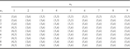
Table 9 The optimal total dividends for 1≤u 1, u 2≤9.

4.2. Examination of the table of the joint dividends
For the rest of the paper, we follow closely the model settings as in Example 2 in section 3.1 with Poisson rates λ 11=λ 22=λ 12=1, i.e., the premium rates are c 1=2.2 and c 2=3.3, the claim pdf’s are ![]() $$f_{{11}} (y)=f_{{1{\bullet}}} (y)=8{\rm e}^{{{\minus}2y}} {\rm sin}^2 y$$
and f 22(y)=f ∙2(y)=(1/4)(0.62ye−0.6y)+(3/4)(92ye−9y) with Z 1 and Z 2 independent, and the force of interest is δ=0.05. The approximation procedures outlined at the beginning of section 2.4 will be applied throughout. Because we will look at larger barrier levels, the smaller scaling factors of (β 1, β 2)=(3, 2) will be applied throughout (see concluding remarks in section 5). As in the fully discrete Example 5, we have tested that the optimal barriers depend on the initial capital levels. Since we use (β 1, β 2)=(3, 2), the initial surplus levels (u 1, u 2) and the barriers (b 1, b 2) (and hence the optimal barriers
$$f_{{11}} (y)=f_{{1{\bullet}}} (y)=8{\rm e}^{{{\minus}2y}} {\rm sin}^2 y$$
and f 22(y)=f ∙2(y)=(1/4)(0.62ye−0.6y)+(3/4)(92ye−9y) with Z 1 and Z 2 independent, and the force of interest is δ=0.05. The approximation procedures outlined at the beginning of section 2.4 will be applied throughout. Because we will look at larger barrier levels, the smaller scaling factors of (β 1, β 2)=(3, 2) will be applied throughout (see concluding remarks in section 5). As in the fully discrete Example 5, we have tested that the optimal barriers depend on the initial capital levels. Since we use (β 1, β 2)=(3, 2), the initial surplus levels (u 1, u 2) and the barriers (b 1, b 2) (and hence the optimal barriers ![]() $$(b_{1}^{{\asterisk}} ,b_{2}^{{\asterisk}} )$$
) in the continuous-time model being approximated can be in the fractional form of e.g.
$$(b_{1}^{{\asterisk}} ,b_{2}^{{\asterisk}} )$$
) in the continuous-time model being approximated can be in the fractional form of e.g. ![]() $$\left( {9{1 \over 3},10{1 \over 2}} \right)$$
. However, for illustrative purposes, we only consider integer values of (u 1, u 2) and (b 1, b 2) for convenience.
$$\left( {9{1 \over 3},10{1 \over 2}} \right)$$
. However, for illustrative purposes, we only consider integer values of (u 1, u 2) and (b 1, b 2) for convenience.
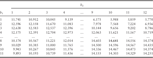
In order to study how the barrier values affect the total expected discounted dividends, we have fixed (u 1, u 2) to be (5, 5), (5, 6) and (5, 7) in turn and then tabulated the approximated total dividend values for various choices of (b 1, b 2) in Tables 10–12. The bold number in each table shows the largest dividend value for its specific combination of (u 1, u 2). We first look at Table 10 for which (u 1, u 2)=(5, 5). If one fixes b 1=1, b 1=2 or b 1=3, then the total dividend value is decreasing in b 2, i.e., b 2=1 gives the largest total dividends. If the value of b 1 is fixed to be larger, then a larger value of b 2 is required to maximise the total dividends. This is also depicted graphically in Figure 1, which plots the approximated total dividends against the barrier value b 2 for each fixed b 1=2, 4, 6, 8, 10, 12. Similar phenomenon is observed if one instead fixes the value of b 2 and varies b 1, and the same is true even when one looks at Tables 11 and 12. This suggests that in order to achieve high joint dividends, the barriers should be fairly close to each other. In addition, as indicated by the bold number in each table, it is found that the maximum total dividend value is achieved at the barriers ![]() $$(b_{1}^{{\asterisk}} ,b_{2}^{{\asterisk}} )$$
=(8, 10) for all three pairs of initial surplus levels considered. This will be further discussed in section 4.3.
$$(b_{1}^{{\asterisk}} ,b_{2}^{{\asterisk}} )$$
=(8, 10) for all three pairs of initial surplus levels considered. This will be further discussed in section 4.3.

Figure 1 Plot of approximated total dividends against b 2 when (u 1, u 2)=(5, 5).
Table 10 Approximated total dividends when (u 1, u 2)=(5, 5).

Table 11 Approximated total dividends when (u 1, u 2)=(5, 6).
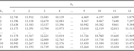
Table 12 Approximated total dividends when (u 1, u 2)=(5, 7).
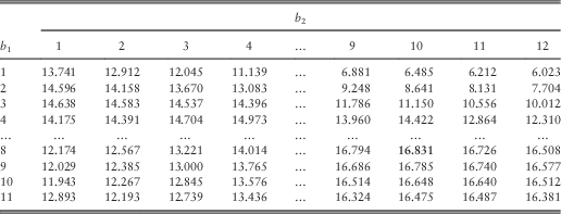
Note that each of Tables 10–12 is divided into four sections: (i) b 1<u 1 and b 2<u 2; (ii) b 1≥u 1 and b 2<u 2; (iii) b 1<u 1 and b 2≥u 2; and (iv) b 1≥u 1 and b 2≥u 2. In the first section, the barrier level is lower than the initial surplus for each line, and therefore each line pays a dividend at time 0 and the bivariate process actually starts at (b 1, b 2). Going from Table 10 to Table 11, the only change is that line 2 possesses one more unit of initial capital, and this explains the fact that each dividend value in Table 11 is exactly one unit larger than the corresponding value in Table 10 within the first section. The same observation applies to Tables 11 and 12 as well. For the second section, the dividend values show the same properties as those in the first section because it is line 2 that pays a dividend at time 0 and then the process starts at (u 1, b 2). In the third section, line 1 (instead of line 2) needs to pay the excess of u 1 over b 2 and then the process starts at (b 1, u 2). In the fourth section, none of the two lines pay out immediate dividends at time 0. Note that all the dividend values in Table 12 are higher than the corresponding ones in Table 11, which are in turn larger than those in Table 10. This is expected since the dividends must be increasing in the initial capital u 2.
4.3. Optimal barriers and restricted optimal barriers
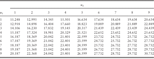
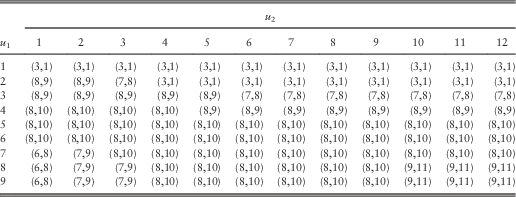
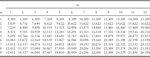
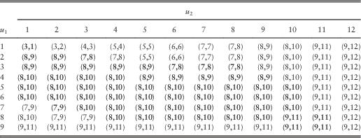
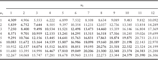
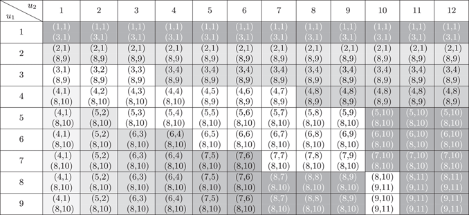
In this section, we are interested in the pair of optimal barriers for every combination of (integer values of) (u 1, u 2) for 1≤u 1≤9 and 1≤u 2≤12. The optimal barriers and the corresponding optimal joint dividend values are given in Tables 13 and 14, respectively.
Table 13 The optimal barriers for 1≤u 1≤9 and 1≤u 2≤12.

Table 14 Approximated optimal dividends for 1≤u 1≤9 and 1≤u 2≤12.

From Table 13, although the optimal barriers ![]() $$(b_{1}^{{\asterisk}} ,b_{2}^{{\asterisk}} )$$
vary with the initial surplus level (u 1, u 2), they often take the value of
$$(b_{1}^{{\asterisk}} ,b_{2}^{{\asterisk}} )$$
vary with the initial surplus level (u 1, u 2), they often take the value of ![]() $$(b_{1}^{{\asterisk}} ,b_{2}^{{\asterisk}} )$$
=(8, 10). The anomalies of lower optimal barriers usually happen when u 1 or u 2 is small. In particular, when line 1 possesses low initial surplus of u 1=1 or u 1=2, the optimal barriers
$$(b_{1}^{{\asterisk}} ,b_{2}^{{\asterisk}} )$$
=(8, 10). The anomalies of lower optimal barriers usually happen when u 1 or u 2 is small. In particular, when line 1 possesses low initial surplus of u 1=1 or u 1=2, the optimal barriers ![]() $$(b_{1}^{{\asterisk}} ,b_{2}^{{\asterisk}} )$$
are mostly the small values of (3, 1). Intuitively, when one of the two lines possesses low initial surplus, the bivariate process is likely to ruin early anyway. To optimise joint dividends, it is important to ensure that some early dividends are paid before ruin (in terms of immediate dividend at time 0 or reaching the barrier early), resulting in lower optimal barriers
$$(b_{1}^{{\asterisk}} ,b_{2}^{{\asterisk}} )$$
are mostly the small values of (3, 1). Intuitively, when one of the two lines possesses low initial surplus, the bivariate process is likely to ruin early anyway. To optimise joint dividends, it is important to ensure that some early dividends are paid before ruin (in terms of immediate dividend at time 0 or reaching the barrier early), resulting in lower optimal barriers ![]() $$(b_{1}^{{\asterisk}} ,b_{2}^{{\asterisk}} )$$
. However, this effect is a bit less obvious when u 2 is low. One possible explanation is that line 2 has a higher security loading (as it has higher premium rate but the same expected claim costs compared to line 1) and hence lower chance of early ruin than line 1, all else being equal. It is also instructive to note that the optimal barriers are always either both high or both low, i.e., it is not optimal for one insurer to set a high barrier if the other one has a low barrier and vice versa. This can be attributed to the fact that dividend payments for both lines cease at the joint ruin time T, and if one of the lines has large positive surplus at time T it would have been better paid as a dividend at the beginning (see section 3.1 for similar comments).
$$(b_{1}^{{\asterisk}} ,b_{2}^{{\asterisk}} )$$
. However, this effect is a bit less obvious when u 2 is low. One possible explanation is that line 2 has a higher security loading (as it has higher premium rate but the same expected claim costs compared to line 1) and hence lower chance of early ruin than line 1, all else being equal. It is also instructive to note that the optimal barriers are always either both high or both low, i.e., it is not optimal for one insurer to set a high barrier if the other one has a low barrier and vice versa. This can be attributed to the fact that dividend payments for both lines cease at the joint ruin time T, and if one of the lines has large positive surplus at time T it would have been better paid as a dividend at the beginning (see section 3.1 for similar comments).
Turning to Table 14, it is clear that the discounted dividend increases with respect to both initial surplus levels. The table can also help us study an optimal allocation problem as well if the criterion is to maximise the total dividends of the two lines. (See also e.g. Loisel, Reference Loisel2005, section 5 or Gong et al., Reference Gong, Badescu and Cheung2012, section 6.3 for discussion of a capital allocation that minimises multivariate risk measures.) Suppose that both business lines belong to a larger corporation who wants to choose (u 1, u 2) to maximise V 1(u 1, u 2; b 1, b 2)+V 2(u 1, u 2; b 1, b 2) subject to the constraint u 1+u 2=K (and of course u 1≥0 and u 2≥0) for a given total initial capital of K>0. This can be regarded as a two-step procedure. First, the optimal pairs of barriers ![]() $$(b_{1}^{{\asterisk}} ,b_{2}^{{\asterisk}} )$$
and the resulting optimal joint dividends are determined as in Tables 13 and 14. Then, we can look at the line u 1+u 2=K in Table 14 to find the optimal combination of
$$(b_{1}^{{\asterisk}} ,b_{2}^{{\asterisk}} )$$
and the resulting optimal joint dividends are determined as in Tables 13 and 14. Then, we can look at the line u 1+u 2=K in Table 14 to find the optimal combination of ![]() $$(u_{1}^{{\asterisk}} ,u_{2}^{{\asterisk}} )$$
that gives the highest dividend value. For easy reference, we additionally plot the optimal joint dividends against the capital u 2 allocated to line 2 given that K=5, 6, 7, 8, 9, 10 in Figure 2. For example, if K=7 then
$$(u_{1}^{{\asterisk}} ,u_{2}^{{\asterisk}} )$$
that gives the highest dividend value. For easy reference, we additionally plot the optimal joint dividends against the capital u 2 allocated to line 2 given that K=5, 6, 7, 8, 9, 10 in Figure 2. For example, if K=7 then ![]() $$u_{2}^{{\asterisk}} =3$$
yields the highest joint dividends and hence
$$u_{2}^{{\asterisk}} =3$$
yields the highest joint dividends and hence ![]() $$u_{1}^{{\asterisk}} =K{\minus}u_{2}^{{\asterisk}} =4$$
; if K=10 then
$$u_{1}^{{\asterisk}} =K{\minus}u_{2}^{{\asterisk}} =4$$
; if K=10 then ![]() $$(u_{1}^{{\asterisk}} ,u_{2}^{{\asterisk}} )=(5,5)$$
(and in both cases
$$(u_{1}^{{\asterisk}} ,u_{2}^{{\asterisk}} )=(5,5)$$
(and in both cases ![]() $$(b_{1}^{{\asterisk}} ,b_{2}^{{\asterisk}} )=(8,10)$$
). It is noted that the optimal allocation
$$(b_{1}^{{\asterisk}} ,b_{2}^{{\asterisk}} )=(8,10)$$
). It is noted that the optimal allocation ![]() $$(u_{1}^{{\asterisk}} ,u_{2}^{{\asterisk}} )$$
appears to occur at places where the total capital K is roughly equally split. The intuitive reason is that if the allocation is at either extreme end, then it is more likely that one of the two lines possesses positive surplus at the joint ruin time T and resources are wasted (see section 3.1).
$$(u_{1}^{{\asterisk}} ,u_{2}^{{\asterisk}} )$$
appears to occur at places where the total capital K is roughly equally split. The intuitive reason is that if the allocation is at either extreme end, then it is more likely that one of the two lines possesses positive surplus at the joint ruin time T and resources are wasted (see section 3.1).

Figure 2 Plot of approximated optimal dividends against u 2 under u 1+u 1=K.
So far, when we maximise the joint dividends we place no restrictions on whether the barriers should be below or above the respective initial surplus levels of the two lines. However, we already know from Table 13 that this could lead to optimal barriers that are much lower than the initial surplus levels, leading to earlier ruin than the case if higher barriers are applied. Practically, early ruin may not be desirable for risk management purposes even dividends are maximised. These lead to the idea of maximising dividends under a penalty at ruin or a ruin probability constraint (see e.g. Dickson & Waters, Reference Dickson and Waters2004; Dickson & Drekic, Reference Dickson and Drekic2006; Gerber et al., Reference Gerber, Shiu and Smith2006; Thonhauser & Albrecher, Reference Thonhauser and Albrecher2007). In the present context, we can delay ruin by maximising the joint dividends under the constraint that the barrier levels should be no less than the respective initial surplus levels. The resulting barrier levels will be called “restricted optimal barriers”. Tables 15 and 16 give the restricted optimal barriers and the resulting joint dividend values, respectively.
Table 15 The restricted optimal barriers for 1≤u 1≤9 and 1≤u 2≤12.

Table 16 Approximated restricted optimal dividends for 1≤u 1≤9 and 1≤u 2≤12.

In both Tables 15 and 16, the numbers in bold correspond to the positions where the values are identical to those in Tables 13 and 14. These cells are mainly where the initial surplus levels are of fairly balanced values. At many other positions, the restricted optimal barriers in Table 15 are much higher than the globally optimal barriers in Table 13. Moreover, since Table 16 is a result of constrained optimisation, its values are no larger than those in Table 14. However, it is instructive to note that except when u 1=1 the dividend values in Table 16 are still comparable to those in Table 14. This suggests that applying the restricted optimal barriers can actually delay ruin (due to higher barriers) without sacrificing much dividends. Nonetheless, Table 15 shows the same phenomenon as in Table 13 that the restricted optimal barriers of the two lines are always of similar values. The intuitive reason is similar to that for the globally optimal barriers. When one turns to the problem of capital allocation based on the restricted optimal barriers, the results of the optimal allocation are identical to the case where the globally optimal barriers are used, at least up to K=10, this is depicted in Figure 3.

Figure 3 Plot of approximated restricted optimal dividends against u 2 under u 1+u 2=K.
4.4. A modified type of barrier strategy
In this section, we shall study a modified type of barrier strategy based on some observations from Table 14 regarding the dividend values under the globally optimal barriers. It has been always assumed that at time 0 the two lines of business fix their barrier levels that will not be changed later on. But if time 0 is a decision time to set the barriers, it would make sense to allow immediate dividends to be paid at time 0 so that the bivariate process moves to a better starting position from which the new globally optimal barriers are implemented.
The above idea can be illustrated with a concrete example as follows. Suppose that the bivariate risk process starts with initial surplus levels (u 1, u 2)=(3, 8). From Tables 13 and 14, we know that the optimal joint dividend value is 14.460 under the optimal barriers (7, 8). However, if line 2 pays an immediate dividend of 1, then the bivariate process moves to the new position (3, 7) and the optimal barriers for the initial surplus levels (3,7) (which happen to be (7, 8) also) can be applied. This will result in higher total joint dividends of 1+13.473=14.473. But if line 2 continues paying an immediate dividend of 1, moving the bivariate process to (3, 6), then the total joint dividends will be even higher at 14.498. The procedure continues, and no further improvement is possible upon reaching position (3, 4) where total joint dividends of 14.534 can be enjoyed. To summarise, starting with (u 1, u 2)=(3, 8), the overall strategy would be for line 2 to pay 4 at time 0, and then implement the barriers (8, 9) so that the expected present value of future dividends is 10.534.
Following the above arguments, we have tabulated the optimal parameters of the modified barrier strategy in Table 17. In each cell, the upper pair is the target starting position while the lower pair represents the optimal barriers for the new starting position. Table 18 gives the dividend values accordingly.
Table 17 Optimal parameters of the modified barrier strategy.

Table 18 Approximated optimal dividends under modified barrier strategy.

First, the cells in Tables 17 and 18 with white background indicate positions (i) where there does not exist any modified barrier strategy that can beat the (globally) optimal barrier strategy in Tables 13 and 14; (ii) that are not the target starting positions for other starting initial surplus levels under consideration; and (iii) that do not involve any immediate dividends at time 0. Second, a (partial) column or row with black numbers and the same grey background in Tables 17 and 18 represents positions that all collapse to the uppermost or leftmost cell within that (partial) column or row. For example, as long as u 1=3 and 4≤u 2≤12, line 2 should pay a dividend of u 2−4 at time 0 and then the two lines should implement (8, 9) as the barriers. As another example, within the group where 5≤u 1≤9 and u 2=2, line 1 immediately pays out u 1−5 and then the two lines apply the barriers (8, 10). Except for the target positions, all these cells with grey background in Table 18 have strictly higher dividend values than the corresponding ones under the (globally) optimal barrier strategy given in Table 14. Finally, each remaining cell with the darkest background and white number actually has the same modified barrier strategy as the (globally) optimal barrier strategy, but the interpretation is slightly more complicated. For example, when u 1=5 and 10≤u 2≤12, Table 13 indicates (globally) optimal barriers of ![]() $$(b_{1}^{{\asterisk}} ,b_{2}^{{\asterisk}} )=(8,10)$$
. Since
$$(b_{1}^{{\asterisk}} ,b_{2}^{{\asterisk}} )=(8,10)$$
. Since ![]() $$u_{2} \geq b_{2}^{{\asterisk}} $$
, this essentially means that line 2 should pay an immediate dividend of u 2−10 (moving the bivariate process to (5, 10)) and continue to apply the barriers (8, 10). Again from Table 13, it is known that the (globally) optimal barriers corresponding to the initial surplus levels (u 1, u 2)=(5, 10) are also (8, 10). Therefore, the above description is indeed identical to the modified strategy given in Table 17, with (5, 10) being the target starting position and (8, 10) the new barriers.
$$u_{2} \geq b_{2}^{{\asterisk}} $$
, this essentially means that line 2 should pay an immediate dividend of u 2−10 (moving the bivariate process to (5, 10)) and continue to apply the barriers (8, 10). Again from Table 13, it is known that the (globally) optimal barriers corresponding to the initial surplus levels (u 1, u 2)=(5, 10) are also (8, 10). Therefore, the above description is indeed identical to the modified strategy given in Table 17, with (5, 10) being the target starting position and (8, 10) the new barriers.
It is instructive to note that the dividend values in Table 18 are no less than those in Table 14 under the (globally) optimal barriers. More importantly, in some cases where the (globally) optimal barriers are low in Table 13, application of our proposed modified barrier strategy can lead to later ruin time as well. For example, when u 1=2 and 4≤u 2≤12, under both strategies in Tables 13 and 17 the bivariate process essentially starts at the initial surplus levels (2, 1) after payment of an immediate dividend at time 0. But the higher barriers of (8, 9) applied under the modified strategy (compared with the barriers (3, 1) in Table 13) mean that the bivariate process can now survive longer. Therefore, our proposed modified strategy could have the advantage of increased joint dividends and delayed ruin time in comparison with the standard barrier strategy. Finally, Figure 4 shows that our modified barrier strategy leads to the same optimal capital allocation as in Figures 2 and 3 for at least up to K=10.

Figure 4 Plot of approximated optimal dividends against u 2 under u 1+u 1=K with the modified barrier strategy.
5. Concluding Remarks
In this paper, a discretisation procedure is developed to approximate a continuous-time bivariate risk process. Applications to related optimal problems in reinsurance, capital allocation and dividends are illustrated with numerical examples. A modified dividend barrier strategy that can lead to increased dividends and longer survival time is proposed.
There are various directions for future research. First, with the barrier levels (b 1, b 2) in the continuous-time model along with the scaling factors (β 1, β 2), one needs to solve a system of (β 1b 1+1)(β 2b 2+1) linear equations in the discrete model according to the approximation procedures outlined at the beginning of section 2.4. In cases where (b 1, b 2) and (β 1, β 2) are both large, the computer can actually run out of memory. (This explains the choices of low barriers in section 3 and low scaling factors in section 4.) More efficient computational methods should be explored. Second, in principle, our procedures can be extended from bivariate to multivariate processes. But the calculations will be far more tedious, and again better algorithms will be needed. Third, the present model may be modified so that capital transfer between lines (e.g. Hult & Lindskog, Reference Hult and Lindskog2006) is possible when one business line is in danger while the other has abundant capital. Finally, one may also attempt to obtain explicit expressions under the simplest model assumptions such as exponential claims with common shocks only or under proportional reinsurance. We leave these as open questions.
Acknowledgements
The authors would like to thank Andrei Badescu, Landy Rabehasaina and two anonymous referees for helpful comments and suggestions that improved an earlier version of the paper. Eric Cheung gratefully acknowledges the support from the CAE 2013 research grant from the Society of Actuaries. Any opinions, finding, and conclusions or recommendations expressed in this material are those of the authors and do not necessarily reflect the views of the SOA.


