A Bayesian smoothing spline method for mortality modelling

Arto Luoma; Anne Puustelli; Lasse Koskinen

doi:10.1017/S174849951200005X

A Bayesian smoothing spline method for mortality modelling

Published online by Cambridge University Press: 15 May 2012

Arto Luoma ,

Anne Puustelli and

Lasse Koskinen

Show author details

Arto Luoma*: Affiliation:
University of Tampere, Finland
Anne Puustelli: Affiliation:
University of Tampere, Finland
Lasse Koskinen: Affiliation:
Financial Supervisory Authority of Finland and Helsinki School of Economics, Finland
*: *Correspondence to: Arto Luoma, School of Information Sciences, FIN-33014 University of Tampere, Finland. E-mail: arto.luoma@uta.fi

Article contents

Abstract
Introduction
Data
Preliminary model
The final model
Estimation
Model checking
Conclusions
Footnotes
References

Rights & Permissions

Abstract

We propose a new method for two-dimensional mortality modelling. Our approach smoothes the data set in the dimensions of cohort and age using Bayesian smoothing splines. The method allows the data set to be imbalanced, since more recent cohorts have fewer observations. We suggest an initial model for observed death rates, and an improved model which deals with the numbers of deaths directly. Unobserved death rates are estimated by smoothing the data with a suitable prior distribution. To assess the fit and plausibility of our models we perform model checks by introducing appropriate test quantities. We show that our final model fulfils nearly all requirements set for a good mortality model.

Keywords

Cohort effect Forecasting Model checking Parameter uncertainty Stochastic mortality model

Type: Papers
Information: Annals of Actuarial Science , Volume 6 , Issue 2 , 23 August 2012 , pp. 284 - 306

DOI: https://doi.org/10.1017/S174849951200005X [Opens in a new window]
Copyright: Copyright © Institute and Faculty of Actuaries 2012

1 Introduction

Mortality forecasting is a problem of fundamental importance for the insurance and pensions industry. Due to the increasing focus on risk management and measurement for insurers and pension funds, stochastic mortality models have attracted considerable interest in recent years. A range of stochastic models for mortality have been proposed, for example the seminal models of Lee & Carter (Reference Lee and Carter1992), Renshaw & Haberman (Reference Renshaw and Haberman2006) and Cairns et al. (Reference Cairns, Blake and Dowd2006b). Some models build on an assumption of smoothness in mortality rates between ages in any given year (e.g. Cairns et al., Reference Cairns, Blake and Dowd2006b), while others allow for roughness, (e.g. Lee & Carter Reference Lee and Carter1992; Renshaw & Haberman, Reference Renshaw and Haberman2006).

In this paper we propose a new Bayesian method for two-dimensional mortality modelling. Our method is based on natural cubic smoothing splines, which are popular in statistical applications, since the smoothing problem can be solved using simple linear algebra. In this approach the distinct data values are taken as knots of the spline, and its smoothness is achieved by employing roughness penalty in a penalized likelihood function. In the Bayesian approach, the prior distribution takes the role of the roughness penalty term. A useful introduction to smoothing splines may be found, for example, in Green & Silverman (Reference Green and Silverman1994).

A more general penalized splines approach would employ a set of basis functions, such as B-splines. In the case that cubic B-splines are used, one may obtain the same solution as in the smoothing spline approach by using the same roughness penalty and by choosing the knots to be the distinct values of the data points. Compared to the general penalized splines approach our approach has the advantage that one does not need to optimize with respect to the number of knots and their locations. However, the drawback in our approach is that the matrices involved in computations become too large, unless one restricts the size of the estimation data set.

We use age-cohort data instead of age-period data, since we wish to preserve the sequential dependence of observations within each cohort. Therefore, we have to deal with imbalanced data, since more recent cohorts have fewer observations. We suggest an initial model for the observed death rates, and an improved model which deals with the numbers of deaths directly. We assume the number of deaths to follow a Poisson distribution, a common model for the number of deaths in a year in a particular cohort. Unobserved death rates are estimated by smoothing the data with one of our spline models. The proposed method is illustrated using Finnish mortality data for females, provided by the Human Mortality Database. We implement the Bayesian approach using the Markov chain Monte Carlo method (MCMC), or more specifically, the single-component Metropolis-Hastings algorithm.

The use of Bayesian methods is not new in this general context. Dellaportas et al. (Reference Dellaportas, Smith and Stavropoulos2001) proposed a Bayesian mortality model in a parametric curve modelling context. Czado et al. (Reference Czado, Delwarde and Denuit2005) and Pedroza (Reference Pedroza2006) provided Bayesian analyses for the Lee-Carter model using MCMC, with further work by Kogure & Kurachi (Reference Kogure and Kurachi2010). More recently, Reichmuth & Sarferaz (Reference Reichmuth and Sarferaz2008) have applied MCMC to a version of the Renshaw & Haberman (Reference Renshaw and Haberman2006) model. Schmid & Held (Reference Schmid and Held2007) present software which allows analysis of incidence count data with a Bayesian age-period-cohort model. Cairns et al. (Reference Cairns, Blake, Dowd, Coughlan and Khalaf-Allah2011) use the same model to compare results based on a two-population approach with single-population results. Currie et al. (Reference Currie, Durban and Eilers2004) and Richards et al. (Reference Richards, Kirkby and Currie2006) assume smoothness in both age and cohort dimensions through the use of P-splines in a non-Bayesian set-up. Lang & Brezger (Reference Lang and Brezger2004) introduce two-dimensional P-splines in a Bayesian set-up but in a different context.

Cairns et al. (Reference Cairns, Blake and Dowd2008) evaluated several types of stochastic mortality models using a checklist of criteria. These criteria are based on general characteristics and the ability of the model to explain historical patterns of mortality. None of the existing models met all of the criteria. However, Plat (Reference Plat2009) later proposed a model which apart from partly meeting the parsimony criteria meets all of the criteria. We also follow the same list in assessing the fit and plausibility of our model.

The plan of the paper is as follows. In the next section we describe the data and its use in estimation. In Section 3 we explain the smoothing problem and present the Bayesian formulation of the preliminary model, and in Section 4 we describe our final model. In Section 5 we introduce the estimation method and provide some convergence results. The model checks are described in Section 6, after which we conclude with a brief discussion.

2 Data

We use mortality data provided by the Human Mortality Database. This was created to provide detailed mortality and population data to those interested in the history of human longevity. In our work we use Finnish cohort mortality data for females. We use age-cohort data instead of age-period data, since we wish to take into account the dependence of consecutive observations within each cohort. In the complete data matrix the years of birth included are between 1807 and 1977; hence there are 171 different cohorts. The most recent data are from 2006. When the age group of persons 110 years and older is excluded, the dimensions of the data matrix become 110 × 171. These data are illustrated in Figure 1, in which the observed area is denoted by vertical lines and the unobserved by two white triangles in the upper left and lower right corners.

Figure 1 Age-cohort representation of the data set. The complete data set is indicated by the streaked area, and the imbalanced estimation set by the white rectangle.

Our estimation method would produce huge matrices if all these data were used simultaneously. Therefore, we define estimation areas which are parts of the complete data set. A rectangular estimation area shown in Figure 1 indicates the cohorts and ages for which a smooth spline surface is fitted. The mortality rates are known for part of this area, and they are predicted for the unknown part. More specifically, an estimation area is defined by minimum age x ₁, maximum age x_K, minimum cohort t ₁ and maximum cohort t_T. The maximum age for which data are available in cohort t_T is denoted as x _*. Thus, the number of ages included is K = x_K − x ₁ + 1 and the number of cohorts T = t_T − t ₁ + 1.

Since the reader might be more familiar with age-period data, we have also plotted the data set in the dimensions of age and year in Figure 2. One should, however, remember that the figures in these two types of mortality tables are not computed in the same way. One figure in an age-period table is based on persons who have a certain (discrete) age during one calendar year and are born during two consecutive years, while each figure in an age-cohort table is based on data from two consecutive calendar years about persons born in a certain year (for details, see Wilmoth et al., Reference Wilmoth, Andreev, Jdanov and Glei2007).

Figure 2 Age-period representation of the data set. The complete data set is indicated by the streaked area, and the imbalanced estimation set by the white parallelogram.

3 Preliminary model

We start building our model in a simplified set-up. Let us denote the logarithms of observed death rates as y_xt = log(m_xt) for ages x = x ₁, x ₂,…, x_K and cohorts (years of birth) t = t ₁, t ₂,…, t_T. The observed death rates are defined as

$--><$$> {{m}_{xt}}\, = \,\frac{{{{d}_{xt}}}}{{{{e}_{xt}}}}, \eqno<$$><!--$

where d_xt is the number of deaths and e_xt the person years of exposure. In our preliminary set-up we model the observed death rates directly, while in our final set-up we model the theoretical, unobserved death rates μ_xt.

3.1 The smoothing problem

Our goal is to smooth and predict logarithms of observed death rates. We fit a smooth two-dimensional curve θ(x,t), and denote its values at discrete points as θ_x _,_t. In matrix form we may write

$--><$$> { {{\bf Y}}}\, = \,\brTheta \, + \,{\bf {{E}}}, \eqno<$$><!--$

where Y is a K × T matrix of observations, Θ is a matrix of smoothed values, and E is a matrix of errors. We denote the columns of Y, Θ and E by y_j, θ_j and ε_j, respectively. Concatenating the columns we obtain y = vec(Y), θ = vec(Θ) and ε = vec(E).

We further assume that the death rates within a cohort follow a multivariate normal distribution having an AR(1) correlation structure with autocorrelation coefficient φ. Thus,

$--><$$>{ \hslant20%{\tf="MPi-Four"\char101}}{{}_j}\, \sim \,N({\bf 0},{{\sigma }^2} {\bf {{P}}}),\; \; j\, = \,1,2, \ldots, T, \eqno<$$><!--$

where P is a correlation matrix with elements $)(--><$> {{\rho }_{rs}}\, = \,{{\phi }^{|r{\rm{ - }}s|}} <$><!--$ . The observations in different cohorts are assumed to be independent.

In general, all observations are not available for all cohorts. For each j, we may partition y_j into observed y_j ₁ and unobserved y_j ₂, and θ_j correspondingly into θ_j ₁ and θ_j ₂, and P into P_j,r,s, r, s = 1,2. The unobserved part of the data can be predicted using the result about the conditional distribution of the multivariate normal distribution:

$--><$$> \{ {{{\bf {{y}}}}_{j2}}\,|\,{{{\bf {{y}}}}_{j1}},{{\sigma }^2}, \phi \} \, \sim \,N({{\bitheta }_{j,2.1}},{{\sigma }^2} {{{\bf {{P}}}}_{j,22.1}}), \eqno<$$><!--$

where $)(--><$> {{\bitheta }_{j,2.1}}\, = \,{{\bitheta }_{j2}}\, + \,{{{\bf {{P}}}}_{j,21}}{\bf {{P}}}_{{j,11}}^{{{\rm{ - }}1}} ({{{\bf {{y}}}}_{j1}}{\rm{ - }}{{\bitheta }_{j1}}) <$><$> {{{\bf {{P}}}}_{j,22.1}}\, = \,{{{\bf {{P}}}}_{j,22}}{\rm{ - }}{{{\bf {{P}}}}_{j,21}}{\bf {{P}}}_{{j,11}}^{{{\rm{ - }}1}} {{{\bf {{P}}}}_{j,12}} <$><!--$ .

When estimating θ we wish to minimize the generalized sum of squares

(1)

$--><$$> S{{S}_1}\, = \,\mathop{\sum}\limits_{j\, = \,1}^T ({{{\bf {{y}}}}_{j1}}{\rm{ - }}{{\bitheta }_{j1}})^{\prime}{\bf {{P}}}_{{j,11}}^{{{\rm{ - }}1}} ({{{\bf {{y}}}}_{j1}}{\rm{ - }}{{{ {{\bitheta}}}}_{j1}}). \eqno<$$><!--$

The vector of all observed mortality rates is y^obs = Sy, where S is a selection matrix selecting the known values from the complete data vector y. The matrix S can be constructed from the identity matrix of size KT by including the ith row (i = 1, 2,…, KT) if the ith element of y is known. Now we can write (1) as

(2)

$--><$$> S{{S}_1}\, = \,({{{\bf {{y}}}}^{obs}} {\rm{ - }}{\bf {{S}}}\bitheta )^{\prime}{{({\bf {{S}}}{{{\bf {{P}}}}_\ast}{\bf {{S}}}')}^{{\rm{ - }}1}} ({{{\bf {{y}}}}^{obs}} {\rm{ - }}{\bf {{S}}}\bitheta ), \eqno<$$><!--$

where P_* = I_T⊗P.

In addition to maximizing fit, we wish to smooth Θ in the dimensions of cohort and age. Specifically, we minimize the roughness functional

(3)

$--><$$> {\int}_{{{{\!\!\!x}_1}}}^{{{{x}_K}}} {{\left[ {\frac{{{{\partial }^2} }}{{\partial {{x}^2} }}\theta (x,{{t}_j})} \right]}^2} dx \eqno<$$><!--$

for each j = 1,2,…,T and

(4)

$--><$$> {\int}_{{{{\!\!\!t}_1}}}^{{{{t}_T}}} {{\left[ {\frac{{{{\partial }^2} }}{{\partial {{t}^2} }}\theta ({{x}_k},t)} \right]}^2} dt \eqno<$$><!--$

for each k = 1,2,…,K.

If θ(x,t_j) is considered a smooth function of x obtaining fixed values at points x _1,x ₂,…, x _K, then using variational calculus it can be shown that the integral in (3) is minimized by choosing θ(x,t_j) to be a cubic splines curve with knots at x _1,x ₂,…, x _K. Furthermore, this integral can be expressed as a squared form $)(--><$> \bitheta _{j}^{{\prime}} {{{\bf {{G}}}}_K}{{\bitheta }_j} <$><$> \bitheta _{{(k)}}^{{\prime}} {{{\bf {{G}}}}_T}{{\bitheta }_k} <$><!--$ , where θ_(k) denotes the kth row of Θ and G_T is a T × T roughness matrix. Thus, we wish to minimize

(5)

$--><$$>S{{S}_2}\, = \,\mathop{\sum}\limits_{j\, = \,1}^T {{\bitheta }^'} _{\!j} \,{{{\bf {{G}}}}_K}{{\bitheta }_j}\, = \,{{\bitheta }^'} ({{{\bf {{I}}}}_T} \otimes {{{\bf {{G}}}}_K})\bitheta \eqno<$$><!--$

and

(6)

$--><$$>S{{S}_3}\, = \,\mathop{\sum}\limits_{k\, = \,1}^K \bitheta _{{(k)}}^{^{\prime}} {{{\bf {{G}}}}_T}{{\bitheta }_{(k)}}\, = \,\bitheta '({{{\bf {{G}}}}_T} \otimes {{{\bf {{I}}}}_K})\bitheta .\eqno<$$><!--$

An N × N roughness matrix is defined as $)(--><$> {{{\bf {{G}}}}_N}\, = \,{{\brnabla }_N}\brDelta _{N}^{{{\rm{ - }}1}} \brnabla _{{N}}^{^{\prime}} <$><$> {{\brnabla }_N} <$><$> {{\brDelta }_N} <$><!--$ , respectively, are defined as follows:

$--><$$>{{\nabla }_{i,i}}\, = \,\frac{1}{{{{x}_{i\, + \,1}}{\rm{ - }}{{x}_i}}},\; \; {{\nabla }_{i\, + \,1,i}}\, = \,{\rm{ - }}\left( {\frac{1}{{{{x}_{i\, + \,1}}{\rm{ - }}{{x}_i}}}\, + \,\frac{1}{{{{x}_{i\, + \,2}}{\rm{ - }}{{x}_{i\, + \,1}}}}} \right),\; \; {{\nabla }_{i\, + \,2,i}}\, = \,\frac{1}{{{{x}_{i\, + \,2}}{\rm{ - }}{{x}_{i\, + \,1}}}}\eqno<$$><!--$

and

$--><$$>{{\rDelta }_{i,i\, + \,1}}\, = \,{{\rDelta }_{i\, + \,1,i}}\, = \,\frac{{{{x}_{i\, + \,2}}{\rm{ - }}{{x}_{i\, + \,1}}}}{6},\; \; {{\rDelta }_{i,i}}\, = \,\frac{{{{x}_{i\, + \,2}}{\rm{ - }}{{x}_i}}}{3},\eqno<$$><!--$

with data points x_i, i = 1,…, n. In our case the data are given at equal intervals, implying that

$--><$$>{{\nabla }_{i,i}}\, = \,1,\; \; {{\nabla }_{i\, + \,1,i}}\, = \,{\rm{ - }}2,\; \; {{\nabla }_{i\, + \,2,i}}\, = \,1\eqno<$$><!--$

and

$--><$$>{{\rDelta }_{i,i\, + \,1}}\, = \,{{\rDelta }_{i\, + \,1,i}}\, = \,\frac{1}{6},\; \; {{\rDelta }_{i,i}}\, = \,\frac{2}{3}.\eqno<$$><!--$

Combining the previous results, we obtain the bivariate smoothing splines solution for θ by minimizing the expression SS ₁ + λ ₁SS ₂ + λ ₂SS ₃, where SS ₁, SS ₂ and SS ₃ are given in the equations (2), (5) and (6), respectively, and the parameters λ ₁ and λ ₂ control smoothing in the dimensions of age and cohort, respectively. Using matrix differentiation and the properties of Kronecker's product, it is easy to show that for fixed values of λ ₁ and λ ₂ the minimal solution is given by

(7)

$--><$$>\hat{\bitheta }\, = \,{{\left[ {{\bf {{S}}}^{\prime}{{{({\bf {{S}}}{{{\bf {{P}}}}_\ast}{\bf {{S}}}^{\prime})}}^{{\rm{ - }}1}} {\bf {{S}}}\, + \,{\bf {{A}}}} \right]}^{{\rm{ - }}1}} {\bf {{S}}}^{\prime}{{({\bf {{S}}}{{{\bf {{P}}}}_\ast}{\bf {{S}}}^{\prime})}^{{\rm{ - }}1}} {{{\bf {{y}}}}^{obs}}, \eqno<$$><!--$

where

(8)

$--><$$>{\bf {{A}}}\, = \,{{\lambda }_1}({{{\bf {{I}}}}_T} \otimes {{{\bf {{G}}}}_K})\, + \,{{\lambda }_2}({{{\bf {{G}}}}_T} \otimes {{{\bf {{I}}}}_K}).\eqno<$$><!--$

In the special case that the data set is balanced (S is an identity matrix), the solution is simplified to $)(--><$> \hat{\bitheta }\, = \,{{({\bf {{I}}}\, + \,{{{\bf {{P}}}}_\ast}{\bf {{A}}})}^{{\rm{ - }}1}} {\bf {{y}}} <$><!--$ .

3.2 Bayesian formulation

Bayesian statistical inference is based on the posterior distribution, which is the conditional distribution of unknown parameters given the data. In order to compute the posterior distribution one needs to define the prior distribution, which is the unconditional distribution of parameters, and the likelihood function, which is the probability density of observations given the parameters. Bayes’ theorem implies that the posterior distribution is proportional to the product of the prior distribution and the likelihood:

$--><$$>p(\bieta \,|\,{\bf {{y}}})\, \propto \,p(\bieta )p({\bf {{y}}}\,|\,\bieta ),\eqno<$$><!--$

where y is the data vector and η the vector of all unknown parameters.

In our case, the likelihood is given by

(9)

$--><$$>p({{{\bf {{y}}}}^{obs}} \,|\,\bieta )\, = \,{{(2\pi {{\sigma }^2} )}^{{\rm{ - }}\frac{{{{K}_\ast}}}{2}}} \,|\,{\bf {{S}}}{{{\bf {{P}}}}_\ast}{\bf {{S}}}^{\prime}\,|{{\,}^{{\rm{ - }}\frac{1}{2}}} {{{\rm{e}}}^{{\rm{ - }}\frac{1}{{2{{\sigma }^2} }}({{{\bf {{y}}}}^{obs}} {\rm{ - }}{\bf {{S}}}\bitheta )^{\prime}{{{({\bf {{S}}}{{{\bf {{P}}}}_\ast}{\bf {{S}}}^{\prime})}}^{{\rm{ - }}1}} ({{{\bf {{y}}}}^{obs}} {\rm{ - }}{\bf {{S}}}\bitheta )}}, \eqno<$$><!--$

where K _* is the length of y^obs.

In order to facilitate estimation we reparametrize the smoothing parameters as follows: λ = λ ₁ and ω = λ ₂/λ ₁, where λ ₁ and λ ₂ control the smoothing in the dimensions of age and cohort, respectively. Furthermore, we use the following hierarchical prior for η:

$--><$$>p(\bieta )\, = \,p({{\sigma }^2} )p(\lambda )p(\omega )p(\phi )p(\bitheta |{{\sigma }^2}, \lambda, \omega, \phi ),\eqno<$$><!--$

where

(10)

$--><$$>\displaylines{ & p({{\sigma }^2} ) \propto \frac{1}{{{{\sigma }^2} }} \cr p(\lambda ) \propto {{\lambda }^{{{\alpha }_1}{\rm{ - }}1}} {{e}^{{\rm{ - }}{{\beta }_1}\lambda }} \cr p(\omega ) \propto {{\omega }^{{{\alpha }_2}{\rm{ - }}1}} {{e}^{{\rm{ - }}{{\beta }_2}\omega }} \cr p(\phi ) \propto 1,\; \; {\rm{ - }}1\, \lt \,\phi \, \lt \,1. \cr}\eqno<$$><!--$

As hyperparameters we set α ₁ = β ₁ = 0.001 and α ₂ = β ₂ = 10. Thus, the prior of σ ² is the standard uninformative improper prior used for positive parameters, and the priors of λ and φ are also fairly uninformative. The prior of ω is instead more informative, having mean 1 and variance 0.1, since we found that the data do not contain enough information about ω, and with a looser prior we would face convergence problems in estimation. We made sensitivity analysis with respect to the prior of λ and found that increasing or decreasing the order of magnitude of α ₁ and β ₁ did not essentially affect the results.

The smoothing effect can now be obtained by choosing a conditional prior for θ which is consistent with the smoothing splines solution. Such a prior contains information only on the curvature, or roughness, of the spline surface, not on its position or gradient. Thus, we assume that $)(--><$> \{ \bitheta |{{\sigma }^2}, \lambda, \omega, \phi \} <$><!--$ is multivarite normal with density

(11)

$--><$$>p(\bitheta \;|\;{{\sigma }^2}, \lambda, \omega, \phi )\, = \,{{(2\pi {{\sigma }^2} )}^{{\rm{ - }}\frac{{KT}}{2}}} {{\left| {\lambda \left[ {({{{\bf {{I}}}}_T} \otimes {{{\bf {{G}}}}_{K,\gamma }}\, + \,\omega ({{{\bf {{G}}}}_T} \otimes {{{\bf {{I}}}}_K})} \right]} \right|}^{\frac{1}{2}}} {{e}^{{\rm{ - }}\frac{\lambda }{{2{{\sigma }^2} }}\bitheta '\left[ {({{{\bf {{I}}}}_T} \otimes {{{\bf {{G}}}}_{K,\gamma }})\, + \,\omega ({{{\bf {{G}}}}_T} \otimes {{{\bf {{I}}}}_K})} \right]\bitheta }}, \eqno<$$><!--$

where G_K _,_γ is a positive definite matrix approximating G_K. More specifically, we define G_K _,_γ = G_K + γ XX′, where γ > 0 can be chosen to be arbitrarily small, and X = (1x) with 1 = (1,…,1)′ and x = (x ₁ ,…, x_K)′. Initially, we use G_K _,_γ instead of G_K, since otherwise p(θ | σ ², λ, ω, φ) would be improper, which would lead to difficulties when deriving the conditional posteriors for λ and ω.

Multiplying the densities in (11) and (9) and picking the factors which include θ we obtain the full conditional posterior for θ up to a constant of proportionality:

(12)

$--><$$>p(\bitheta |{\bf {{y}}},{{\sigma }^2}, \lambda, \omega, \phi )\, \propto \:{\rm e}{{\:}^{{\rm{ - }}\frac{1}{{2{{\sigma }^2} }}\left\{ {({{{\bf {{y}}}}^{obs}} {\rm{ - }}{\bf {{S}}}\bitheta )^{\prime}{{{({\bf {{S}}}{{{\bf {{P}}}}_\ast}{\bf {{S}}}')}}^{{\rm{ - }}1}} ({{{\bf {{y}}}}^{obs}} {\rm{ - }}{\bf {{S}}}\bitheta )\, + \,\lambda \bitheta '\left[ {({{{\bf {{I}}}}_T} \,\otimes \,{{{\bf {{G}}}}_{K,\gamma }})\, + \,\omega ({{{\bf {{G}}}}_T} \,\otimes \,{{{\bf {{I}}}}_K})} \right]\bitheta } \right\}}} .\eqno<$$><!--$

Manipulating this expression and replacing G_K,γ with G_k we obtain

$--><$$>p(\theta \,|\,{\bf {{y}}},{{\sigma }^2}, \lambda, \omega, \phi ) \propto \:{\rm{e}}{{\:}^{{\rm{ - }}\frac{1}{{2{{\sigma }^2} }}(\theta {\rm{ - }}\hat{\theta })^{\prime}{\bf {{B}}}(\theta {\rm{ - }}\hat{\theta })}}, \eqno<$$><!--$

where $)(--><$> \hat{\bitheta } <$><$> {\bf {{B}}}\, = \,{\bf {{A}}}\, + \,{\bf {{S}}}^{\prime}{{({\bf {{S}}}{{{\bf {{P}}}}_\ast}{\bf {{S}}}^{\prime})}^{{\rm{ - }}1}} {\bf {{S}}} <$><$> \hat{\bitheta } <$><$> {{{\bf {{G}}}}_{K,\gamma }} \rightarrow {{{\bf {{G}}}}_K} <$><!--$ . This implies that the conditional posterior mode for θ is equal to the smoothing splines solution provided in the previous section. Thus, using the multivariate prior described above, we can implement the roughness penalty of smoothing splines in the Bayesian framework.

In order to implement estimation using the Gibbs sampler, the full conditional posterior distributions of the parameters are needed. In the following, we will provide these for σ ², λ, ω and φ in the limiting case when $)(--><$> {{{\bf {{G}}}}_{K,\gamma }}\, \rightarrow \,{{{\bf {{G}}}}_K} <$><!--$ .

The conditional posterior of σ ² is

$--><$$>p({{\sigma }^2} \,|\,{\bf {{y}}},\lambda, \omega, \phi ) \propto {{({{\sigma }^2} )}^{{\rm{ - }}\left( {\frac{{{{K}_\ast}\, + \,KT}}{2}\, + \,1} \right)}} \:{\rm{e}}{{\:}^{{\rm{ - }}\frac{1}{{2{{\sigma }^2} }}\left[ {({{{\bf {{y}}}}^{obs}} {\rm{ - }}{\bf {{S}}}\bitheta )^{\prime}{{{({\bf {{S}}}{{{\bf {{P}}}}_\ast}{\bf {{S}}}^{\prime})}}^{{\rm{ - }}1}} ({{{\bf {{y}}}}^{obs}} {\rm{ - }}{\bf {{S}}}\bitheta )\, + \,{ {{\bitheta}}}^{\prime}{\bf {{A}}}\bitheta } \right]}}, \eqno<$$><!--$

which is the density of the scaled inverted χ ² -distribution $)(--><$> {\rm{Inv - }}\:{{\chi }^2} (\nu, b) <$><$> b\, = \,(S{{S}_1}\, + \,\lambda S{{S}_2}\, + \,\lambda \omega S{{S}_3})/\nu <$><!--$ with SS ₁, SS ₂ and SS ₃ given in (2), (5) and (6).

The conditional posterior of λ is

(13)

$--><$$>p(\lambda \,|\,{\bf {{y}}},\bitheta, {{\sigma }^2}, \omega, \phi ) \propto {{\lambda }^{{{\alpha }_1}{\rm{ - }}1\, + \,\frac{{KT}}{2}}} \: {\rm e}{{\:}^{{\rm{ - }}\lambda \left[ {{{\beta }_1}\, + \,\frac{1}{{2{{\sigma }^2} }}\bitheta ^{\prime}({{{\bf {{I}}}}_T} \otimes {{{\bf {{G}}}}_K}\, + \,\omega {{{\bf {{G}}}}_T} \otimes {{{\bf {{I}}}}_K})\bitheta } \right]}}, \eqno<$$><!--$

which is the density of Gamma $)(--><$> ({{\alpha }_1}\, + \,KT\,/\,2,\;{{\beta }_1}\, + \,(S{{S}_2}\, + \,\omega S{{S}_3})\,/\,(2{{\sigma }^2} )) <$><!--$ .

The conditional posterior of ω is

(14)

$--><$$>p(\omega \,|\,{\bf {{y}}},\bitheta, {{\sigma }^2}, \lambda, \phi )\, \propto \,{{\omega }^{{{\alpha }_2}\, + \,T{\rm{ - }}2}} {{\left[ {\prod\limits_{k\, = \,1}^{K\,{\rm{ - }}\,2} \prod\limits_{j\, = \,1}^{T{\rm{ - }}2} \left( {1\, + \,\omega \frac{{{{\mu }_j}}}{{{{\nu }_k}}}} \right)} \right]}^{\frac{1}{2}}} \:{\rm{e}}{{\:}^{{\rm{ - }}\omega \left[ {{{\beta }_2}\, + \,\frac{\lambda }{{2{{\sigma }^2} }}\bitheta ^{\prime}({{{\bf {{G}}}}_T} \otimes {{{\bf {{I}}}}_K})\bitheta } \right]}}, \eqno<$$><!--$

where μ_j, j = 1,…, T−2 and v_K, k = 1,…, K−2, are the nonzero eigenvalues of G_T and G_K, respectively. This is not a standard distribution, but since it is log-concave, it is possible to generate values from it using adaptive rejection sampling, introduced by Gilks & Wild (Reference Gilks and Wild1992).

Finally, the conditional posterior of φ, given by

$--><$$>p(\phi |{\bf {{y}}},\bitheta, {{\sigma }^2}, \lambda, \omega ) \propto {{(1{\rm{ - }}{{\phi }^2} )}^{{\rm{ - }}\frac{1}{2}({{K}_\ast}{\rm{ - }}T)}} \:{\rm{e}}{{\:}^{{\rm{ - }}\frac{1}{{2{{\sigma }^2} }}({{{\bf {{y}}}}^{obs}} {\rm{ - }}{\bf {{S}}}\bitheta )^{\prime}{{{({\bf {{S}}}{{{\bf {{P}}}}_\ast}{\bf {{S}}}')}}^{{\rm{ - }}1}} ({{{\bf {{y}}}}^{obs}} {\rm{ - }}{\bf {{S}}}\bitheta )}}, \eqno<$$><!--$

is not of standard form, and it is therefore difficult to generate random variates from it directly. Instead, we may employ a Metropolis step within the Gibbs sampler.

Now, the estimation algorithm is implemented so that the parameters λ, ω, σ ² and θ are updated one by one using Gibbs steps, and φ is updated using a Metropolis step. Further details will be given in Section 5.

4 The final model

In our final set-up we are able to control for unsystematic mortality risk in addition to systematic risk. Unsystematic risk means that even if the true mortality rate were known, the numbers of deaths would remain unpredictable. When the population becomes larger, the unsystematic mortality risk becomes smaller due to diversification.

4.1 Formulation and estimation

In the final model the inference is rendered more accurate by modelling the observed numbers of deaths directly. Specifically, we assume that

$--><$$>{{d}_{xt}}\, \sim \,{\rm{Poisson}}({{{\rm{\mu }}}_{xt}}{{e}_{xt}}),\eqno<$$><!--$

where d_xt is the number of deaths at age x and cohort t, μ_xt is the theoretical death rate (also called intensity of mortality or force of mortality) and e_xt is the person years of exposure. This is an approximation, since neither the death rate nor the exposure is constant during any given year. Our purpose is to model θ_xt = log(μ_xt) with a smooth spline surface. Compared to the preliminary model we have replaced m_xt with μ_xt and removed the error term and its autocorrelation structure.

Similarly to the preliminary model, we obtain the smoothing effect by using a suitable conditional prior distribution for θ. Specifically, we obtain p(θ|λ,ω) by replacing σ ² with 1 in equation (11). For λ and ω we use the same prior distributions as earlier, given by (10), and their conditional posteriors are obtained from (13) and (14) when σ ² is set at 1. However, here we use hyperparameters α ₁ = β ₁ = 10⁻⁶, since removing σ ² changes the scale of λ several orders of magnitude.

Now the full conditional posterior distribution of θ may be written as

(15)

$--><$$> p(\bitheta |{{{\bf {{d}}}}^{obs}}, \lambda, \omega )\, \propto \,\exp \left\{ {\mathop{\sum}\limits_{t\, = \,{{t}_1}}^{{{t}_T}} \mathop{\sum}\limits_{x\, = \,{{x}_1}}^{{{x}_{{{K}_t}}}} \left[ {{{d}_{xt}}{{\theta }_{xt}}{\rm{ - }}{{e}_{xt}}\exp ({{\theta }_{xt}})} \right]{\rm{ - }}\frac{1}{2}\bitheta '{\bf {{A}}}\bitheta } \right\}, \eqno<$$><!--$

where d^obs is a vector of observed death numbers, and K_t the number of ages for which data are available in cohort t. The double sum in this expression comes from the likelihood function and the squared form from the prior distribution.

This model can be estimated similarly to the preliminary model, using Gibbs sampling. However, since the conditional distribution in (15) is non-standard, it is difficult to sample from it directly. Here we may use a Metropolis-Hastings step within the Gibbs sampler. As a proposal distribution we may use a multivariate normal approximation to (15), given by

$--><$$>J(\bitheta |\lambda, \omega )\, \propto \,\exp \left\{ {{\rm{ - }}\frac{1}{2}\left( {{{{\bf {{y}}}}^{obs}} {\rm{ - }}{\bf {{S}}}\bitheta } \right){{{\left( {{\bf {{S}}}\rSigma {\bf {{S}}}^{\prime}} \right)}}^{{\rm{ - }}1}} \left( {{{{\bf {{y}}}}^{obs}} {\rm{ - }}{\bf {{S}}}\bitheta } \right){\rm{ - }}\frac{1}{2}\bitheta '{\bf {{A}}}\bitheta } \right\},\eqno<$$><!--$

where y^obs is a vector of observed log death rates, $)(--><$> \brSigma <$><$> {{v}_{xt}},\;x\, = \,{{x}_1}, \ldots, {{x}_K},\;t\, = \,{{t}_1}, \ldots, {{t}_T}, <$><$> {{v}_{xt}}\, = \,1\,/\,({{e}_{xt}}\exp ({{\tilde{\bitheta }}_{xt}})) <$><$> {{\tilde{\bitheta }}_{xt}}\, = \,(\mathop{\sum}\nolimits_{i\, = \,{\rm{ - }}1}^1 \mathop{\sum}\nolimits_{j\, = \,{\rm{ - }}1}^1 {{y}_{x\, + \,i,t\, + \,j}})\,/\,9 <$><!--$ is an initial approximation to the log death rate.

Thus, the proposal θ* is distributed as

$--><$$>{{\bitheta }^\ast} \, \sim \:{\rm{MVN}}({{{\bf {{C}}}}^{{\rm{ - }}1}} {\bf {{S}}}^{\prime}{{({\bf {{S}}}{\rm{\brSigma }}{\bf {{S}}}^{\prime})}^{{\rm{ - }}1}} {{{\bf {{y}}}}^{obs}}, {{{\bf {{C}}}}^{{\rm{ - }}1}} ),\eqno<$$><!--$

where C = A + S′(SΣS′)⁻¹S, and is accepted with probability

$--><$$>\min \left( {1,\frac{{p({{\bitheta }^\ast} \,|\,{{{\bf {{d}}}}^{obs}}, \lambda, \omega )/J({{\bitheta }^\ast} \,|\,\lambda, \omega )}}{{p(\bitheta \,|\,{{{\bf {{d}}}}^{obs}}, \lambda, \omega )/J(\bitheta \,|\,\lambda, \omega )}}} \right).\eqno<$$><!--$

The whole algorithm is once more a special case of the single-component Metropolis-Hastings. Further details on this algorithm will be provided in the next section.

5 Estimation

5.1 Estimation procedure

Our estimation procedure is a single-component (or cyclic) Metropolis-Hastings algorithm. This is one of the Markov Chain Monte Carlo (MCMC) methods, which are useful in drawing samples from posterior distributions. Generally, MCMC methods are based on drawing values from approximate distributions and then correcting these draws to better approximate the target distribution, and hence they are used when direct sampling from a target distribution is difficult. A useful reference for different versions of MCMC is Gilks et al. (Reference Gilks, Richardson and Spiegelhalter1996).

The Metropolis-Hastings algorithm was introduced by Hastings (Reference Hastings1970) as a generalization of the Metropolis algorithm (Metropolis et al., Reference Metropolis, Rosenbluth, Rosenbluth, Teller and Teller1953). Also the Gibbs sampler proposed by Geman & Geman (Reference Geman and Geman1984) is its special case. The Gibbs sampler assumes the full conditional distributions of the target distribution to be such that one is able to generate random numbers or vectors from them. The Metropolis and Metropolis-Hastings algorithms are more flexible than the Gibbs sampler; with them one only needs to know the joint density function of the target distribution with density p(θ) up to a constant of proportionality.

With the Metropolis algorithm the target distribution is generated as follows: first a starting distribution p ₀(θ) is assigned, and from it a starting-point θ ⁰ is drawn such that p(θ ⁰) > 0. For iterations t = 1,2,…, a proposal θ* is generated from a jumping distribution $)(--><$> J({{\theta }^\ast} \,|\,{{\theta }^{t{\rm{ - }}1}} ) <$><$> J({{\theta }_a}\,|\,{{\theta }_b})\, = \,J({{\theta }_b}\,|\,{{\theta }_a}) <$><!--$ for all θ_a and θ_b. Finally, iteration t is completed by calculating the ratio

(16)

$--><$$>r\, = \,\frac{{p({{\theta }^\ast} )}}{{p({{\theta }^{t{\rm{ - }}1}} )}}\eqno<$$><!--$

and by setting the new value at

$--><$$>{{\theta }^t} \, = \,\left\{ {\matrix{ {{{\theta }^\ast} } \hfill & {\rm with\;probability\;min\:(r,1)} \hfill \cr {{{\theta }^{t{\rm{ - }}1}} } \hfill & {\rm otherwise .} \hfill \right\eqno<$$><!--$

It can be shown that, under mild conditions, the algorithm produces an ergodic Markov Chain whose stationary distribution is the target distribution.

Metropolis-Hastings algorithm generalizes the Metropolis algorithm by removing the assumption of symmetric jumping distribution. The ratio r in (16) is replaced by

$--><$$>r\, = \,\frac{{p({{\theta }^\ast} )\,/\,J({{\theta }^\ast} |{{\theta }^{t{\rm{ - }}1}} )}}{{p({{\theta }^{t{\rm{ - }}1}} )\,/\,J({{\theta }^{t{\rm{ - }}1}} |{{\theta }^\ast} )}}\eqno<$$><!--$

to correct for the asymmetry in the jumping rule.

In the single-component Metropolis-Hastings algorithm the simulated random vector is divided into components or subvectors which are updated one by one. If the jumping distribution for a component is its full conditional posterior distribution, the proposals are accepted with probability one. In the case that all the components are simulated in this way, the algorithm is called a Gibbs sampler. As stated above, in the case of our preliminary model we can simulate all parameters except φ directly, and may therefore use a Gibbs sampler with one Metropolis step. As the jumping distribution of φ we use the normal distribution N(φ ^t−1,0.05²). For the final model we use a Gibbs sampler with one Metropolis-Hastings step for θ. The proposal distribution and its acceptance probability were already given in Section 4.

5.2 Empirical results

All the computations in this article were performed and figures produced using the R computing environment (R Development Core Team, 2010). The functions and data needed to replicate the results can be found at http://mtl.uta.fi/codes/mortality. A minor drawback is that we cannot use all available data in estimation but must restrict ourselves to a relevant subset. This is due to the huge matrices involved in computations if many ages and cohorts are included in the data set. For example, if we used our complete data set, whose dimensions are T = 110 and K = 171, we would have to deal with Kronecker product matrices of dimension 18810 × 18810. This would require 5 GB of memory for storing one matrix and much more for computations. Although we can alleviate the storage problem and also speed up the computations using sparse matrix methods, we still cannot use the complete data set. In our implementation we use the R package SparseM.

To assess the convergence of the simulated Markov chain to its stationary distribution we used 5 representative values of θ, denoted as θ ₁,…,θ ₅, from each corner and the middle of the data matrix, in addition to the upper level parameters. The value θ ₅ is in the lower right corner of the matrix and corresponds to an unobserved data item.

For each data set and both models we assessed the convergence of iterative simulation using three simulated sequences with 5000 iterations. In the case of the final model we discarded 1500 first iterations of each chain as a burn-in period, while in the case of the preliminary model the convergence was more rapid and we discarded only 200 iterations.

Figure 3 shows one simulated chain corresponding to the final model and the data set with ages 50–90 and cohorts 1901–1941. The series of λ and ω do not mix well, that is, they are fairly autocorrelated. To obtain accurate results for the estimates, more iterations would be needed. However, the chains converge to their stationary distribution fairly quickly, as indicated by the values of the potential scale reduction factor, which is a convergence diagnostic introduced by Gelman & Rubin (Reference Gelman and Rubin1992). The diagnostic values for the final model are less than 1.1 indicating approximate convergence. Summaries of the estimation results for both preliminary and final model as well as the diagnostics are provided in Appendix 1.

Figure 3 Posterior simulations of the final model.

6 Model checking

Cairns et al. (Reference Cairns, Blake and Dowd2008) provide a checklist of criteria against which a stochastic mortality model can be assessed. We will follow this list as we assess the fit and plausibility of our two models. The list is as follows:

1. Mortality rates should be positive.
2. The model should be consistent with historical data.
3. Long-term dynamics under the model should be biologically reasonable.
4. Parameter estimates should be robust relative to the period of data and range of ages employed.
5. Model forecasts should be robust relative to the period of data and range of ages employed.
6. Forecast levels of uncertainty and central trajectories should be plausible and consistent with historical trends and variability in mortality data.
7. The model should be straightforward to implement using analytical methods or fast numerical algorithms.
8. The model should be relatively parsimonious.
9. It should be possible to use the model to generate sample paths and calculate prediction intervals.
10. The structure of the model should make it possible to incorporate parameter uncertainty in simulations.
11. At least for some countries, the model should incorporate a stochastic cohort effect.
12. The model should have a non-trivial correlation structure.

Both of our models fulfil the first item in the list, since we model log death rates. To assess the consistency of the models with historical data we will introduce three Bayesian test quantities in Section 6.1.

A model is defined by Cairns et al. (Reference Cairns, Blake and Dowd2006a) to be biologically reasonable if the mortality rates are increasing with age and if there is no long-run mean reversion around a deterministic trend. Our spline approach implies that the log death rate increases linearly beyond the estimable region. The preliminary model allows for short-term mean reversion (or autocorrelation) for the observed death rate, while there is no mean reversion at all in the final model.

The fourth and fifth points in the list, that is, the robustness of parameter estimates and model forecasts, will be studied in Sections 6.2 and 6.3. The figures of posterior predictions in Section 6.3 help assess the plausibility and uncertainty of forecasts and their consistency with historical trends and variability.

Implementing the models is fairly straightforward but involves several algorithms. Basically, we use the Gibbs sampler, and supplement it with rejection sampling and Metropolis and Metropolis-Hastings steps, which are needed to update certain parameters or parameter blocks. A further complication is that we have to use sparse matrix methods to increase the maximum size of the data set.

In the Bayesian approach one typically uses posterior predictive simulation, in which parameter uncertainty is taken into account, to generate sample paths and calculate prediction intervals. This will be explained in detail in Section 6.3.

The hierarchical structure of the spline models makes them parsimonious: on the upper level the preliminary model has 4 parameters, the final model only 2. Both models also incorporate a stochastic cohort effect. The preliminary model incorporates an AR(1) structure for observed mortality, while the final model has no correlation structure for deviations from the spline surface.

One should note, however, that the spline model in itself implies a covariance structure. In the one-dimensional case the Bayesian smoothing spline model can be interpreted as a sum of a linear trend and integrated Brownian motion (Wahba, Reference Wahba1978). The prior distribution does not contain information on the intercept or slope of the trend but implies the covariance structure of the integrated Brownian motion. Similarily, in our two-dimensional case, the spline surface can be interpreted as a sum of a plane and deviations from this plane. The conditional prior of θ, given the smoothing parameters, does not include information on the plane but implies a specific spatial covariance structure for the deviations.

6.1 Tests for the consistency of the model

In the Bayesian framework, posterior predictive simulations of replicated data sets may be used to check the model fit (see Gelman et al., Reference Gelman, Carlin, Stern and Rubin2004). Once several replicated data sets y ^rep have been produced, they may be compared with the original data set y. If they look similar to y, the model fits.

The discrepancy between data and model can be measured using arbitrarily defined test quantities. A test quantity T(y,θ) is a scalar summary of parameters and data which is used to compare data with predictive simulations. If the test quantity depends only on data and not on parameters, then it is said to be a test statistic. If we already have N posterior simulations θ_i, i = 1,…, N, we can generate one replication $)(--><$> y_{i}^{{rep}} <$><$> T(y_{i}^{{rep}}, {{\theta }_i}) <$><$> (T(y,{{\theta }_i}),T(y_{i}^{{rep}}, {{\theta }_i})),\;i\, = \,1, \ldots, N, <$><!--$ where the same scale is used for both coordinates. Further details on this approach can be found in Chapter 6 of Gelman et al. (Reference Gelman, Carlin, Stern and Rubin2004) or Chapter 11 of Gilks et al. (Reference Gilks, Richardson and Spiegelhalter1996).

In the case of our preliminary model, a replication of data is generated as follows: First, θ, σ ² and φ are generated from their joint posterior distribution. Then, using these parameter values, a replicated data vector y^rep is generated from the multivariate normal distribution $)(--><$> N(\theta, {\bf {{I}}} \otimes {{\sigma }^2} {\bf {{P}}}) <$><!--$ . Finally, the elements of y^rep which correspond to the observed values in y^obs are selected. In the case of the final model, θ is first generated and then the numbers of deaths d_xt and exposures e_xt are generated recursively by starting from the smallest age included in the estimation data set. The numbers for the smallest age are not generated but they are taken to be the same as in the estimation set. Finally, the replicated death rates are computed as y_xt = log(d_xt/e_xt), and the values corresponding to the observed values in y^obs are selected. Further details about this procedure are provided in Appendix 2.

We introduce three test quantities to check the model fit. The first measures the autocorrelation of the observed log death rate and the second and third its mean square error:

$--><$$>AC(y,\bitheta )\, = \,\frac{{\mathop{\sum}\limits_{t\, = \,{{t}_1}}^{{{t}_T}} \, \mathop{\sum}\limits_{x\, = \,{{x}_1}}^{{{x}_K}{\rm{ - }}1} ({{y}_{x\, + \,1,t}}{\rm{ - }}{{\theta }_{x\, + \,1,t}})({{y}_{xt}}{\rm{ - }}{{\theta }_{xt}})}}{{\mathop{\sum}\limits_{t\, = \,{{t}_1}}^{{{t}_T}} {{K}_t}}},\eqno<$$><!--$

where K_t is the number of observations in cohort t, and

$--><$$>MS\,{{E}_1}(y,\bitheta )\, = \,\frac{{\mathop{\sum}\limits_{t\, = \,{{t}_1}}^{{{t}_T}} \,\mathop{\sum}\limits_{x\, = \,{{x}_1}}^{{{x}_{{{K}_t}}}} {{{\left( {{{y}_{xt}}{\rm{ - }}{{\theta }_{xt}}} \right)}}^2} }}{{\mathop{\sum}\limits_{t\, = \,{{t}_1}}^{{{t}_T}} {{K}_t}}},\quad MS\,{{E}_2}(y,\bitheta )\, = \,\frac{{\mathop{\sum}\limits_{t\, = \,{{t}_1}}^{{{t}_T}} {{{\left( {{{y}_{{{x}_{{{K}_t}}}t}}{\rm{ - }}{{\theta }_{{{x}_{{{K}_t}}}t}}} \right)}}^2} }}{T}.\eqno<$$><!--$

Figure 4 and 5 show the results when using the data set with ages 50–90 and cohorts 1901–1941. Each figure is based on 500 simulations. If the original data and replicated data were consistent, about half the points in the scatter plot would fall above the 45° line and half below. Figure 4(a) indicates that the preliminary model adequately explains the autocorrelation observed in the original data set, while Figure 5(a) suggests that there might be slight negative autocorrelation in the residuals not explained by the model. However, since the Bayesian p-value, which is the proportion of points above the line, is approximately 0.95, there is no sufficient evidence to reject the assumption of independent Poisson observations.

Figure 4 Goodness-of-fit testing for the preliminary model. (a) Autocorrelation test. (b) MSE test.

Figure 5 Goodness-of-fit testing for the final model. (a) Autocorrelation test. (b) MSE test.

The test statistic MS E ₁ measures the overall fit of the models, and both models pass it (figures not shown). The test statistic MS E ₂ measures the fit at the largest ages of the cohorts. From Figure 5(b) we see that the final model passes this test. However, Figure 4(b) suggests that under the preliminary model the MS E ₂ simulations based on the original data are smaller than those based on replicated data sets (p_B = 0.98). The reason here is that the homoscedasticity assumption of logarithmic mortality data is not valid. The validity of the homoscedasticity and independence assumptions could be further assessed by plotting the standardized residuals (not shown here).

6.2 Robustness of the parameter estimates

The robustness of the parameters may be studied by comparing the posterior distributions when two different but equally sized data sets are used. Here we used two data sets with ages 40–70 and 60–90, and cohorts 1917–1947 and 1886–1916, respectively. We refer to these as the younger and older age groups, respectively. Figure 6 (c) indicates that the variance parameter σ ² of the preliminary model is clearly higher for the younger age group. This results from the fact that the variance of observed log mortality becomes smaller when the age grows. This also causes a robustness problem for λ, since its posterior distribution is dependent on that of σ ². Also φ seems to be somewhat unrobust.

Figure 6 Distributions of (a) λ, (b) ω, (c) σ ² and (d) φ for the preliminary model. The solid line corresponds to the younger (ages 40–70) and the dashed line the older (ages 60–90) age group.

Figure 7 (a) indicates that under the final model the posterior of λ is more concentrated on small values for the older age group. This is compensated by smaller values of ω for the younger group, which indicates that the smoothing effect in the cohort dimension is similar in both groups. However, the difference between the age groups is not as clear as in the case of the preliminary model. Besides, the range of the distribution is fairly large in both cases.

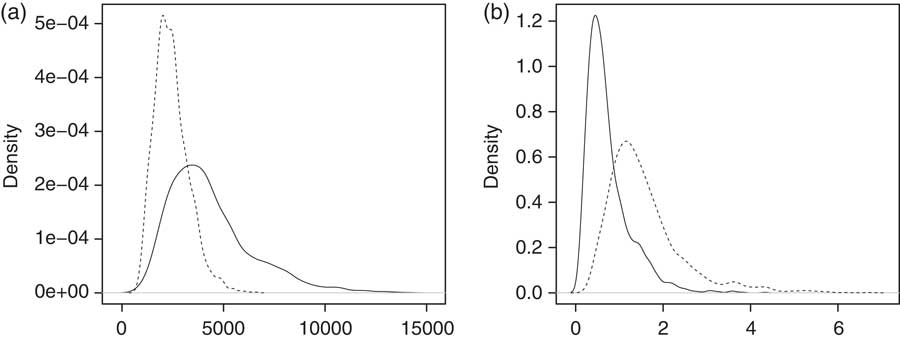
Figure 7 Distributions of (a) λ and (b) ω for the final model. The solid line corresponds to the younger (ages 40–70) and the dashed line the older (ages 60–90) age group.

6.3 Forecasting

Our procedure for forecasting mortality is as follows. We first select a rectangular estimation area which includes in its lower right corner the ages and cohorts for which the death rates are to be predicted. Thus we have in our estimation set earlier observations from the same age as the predicted age and from the same cohort as the predicted cohort. An example of an estimation area is shown in Figure 1.

In the Bayesian approach, forecasting is based on the posterior predictive distribution. In the case of our preliminary model, a simulation from this distribution is drawn as follows: First, θ, σ ² and φ are generated from their joint posterior distribution. Then the unobserved data vectors y_j ₂, j = 1,2,…,T, (which are to be predicted) are generated from their conditional multivariate normal distributions, given the observed data vectors y_j ₁ and the parameters θ, σ ² and φ. These distributions were provided in Section 3. In the case of our final model, θ is first generated. Then the numbers of deaths d_xt and the exposures e_xt are generated recursively starting from the most recent observed values within each cohort. In this way we obtain simulation paths for each cohort and a predictive distribution for each missing value in the mortality table. Further details are provided in Appendix 2.

In studying the accuracy and robustness of forecasts, we use estimation areas similar to those used earlier. However, we choose them so that we can compare the predictive distribution of the death rate with its realized value. The estimation is done as if the triangular area in the right lower corner of the estimation area, indicated in Figure 1, were not known. The posterior predictive distributions shown in Figure 8 are based on the preliminary model, while those in Figure 9 are based on the final model. The four cases in both figures correspond to forecasts 1, 9, 17 and 25 years ahead, for cohorts 1892, 1900, 1908 and 1916, respectively, when the death rate at ages 70 and 90 are forecast. The distributions indicated by solid lines are based on larger estimation sets than those indicated by dashed lines.

Figure 8 Posterior predictive distributions of the death rates at ages 70 and 90, based on the preliminary model. The solid curves correspond to the larger data set (cohorts 1876–1916, and ages 30–70 when the death rate at age 70 is predicted, and ages 50–90 when the death rate at age 90 is predicted) and the dashed curves the smaller (cohorts 1886–1916, and ages 40–70 when the death rate at age 70 is predicted, and ages 60–90 when the death rate at age 90 is predicted). The vertical lines indicate the realized death rates.

Figure 9 Posterior predictive distributions of the death rates at ages 70 and 90, based on the final model. The solid curves correspond to the larger data set (cohorts 1876–1916; ages 30–70 when the death rate at age 70 is predicted, and ages 50–90 when the death rate at age 90 is predicted) and the dashed curves the smaller (cohorts 1886–1916; ages 40–70 when the death rate at age 70 is predicted, and ages 60–90 when the death rate at age 90 is predicted). The vertical lines indicate the realized death rates.

It may be seen that increasing uncertainty is reflected by the growing width of the distributions. Furthermore, the size of the estimation set does not considerably affect the distributions when the death rate at age 90 is predicted, while when it is predicted at age 70, the smaller data sets produce more accurate distributions. The obvious reason is that in the latter case the larger estimation set contains observations from the age interval 30–40 in which the growth of mortality is less regular than at larger ages, inducing more variability in the estimated model. In all cases, the realized values lie within the 90% prediction intervals.

Figure 10 and 11 show posterior predictive simulations for the log death rate when the preliminary and the final model is used, respectively. In each case, the estimation region includes cohorts 1901–1941 and ages 35–100. Three paths of posterior simulations are shown for cohort 1941, for which the data are available until age 65. As may be seen, the variability of the predictions resembles that of the observed path. Furthermore, the 95% posterior limits for the log death rate (θ_xt) and the 95% posterior predictive limits for the observed log death rate (y_xt) are shown. These two types of limits differ substantially only in the beginning of the forecast horizon. The prediction belt is narrower for the final model, which reflects better model fit.

Figure 10 Posterior predictions with the preliminary model for ages 66−100 and cohort 1941. The solid lines represents the 95% posterior limits for θ, the dotted lines the 95% posterior predictive limits for the observed log death rate, and the dashed lines the observed log death rate for ages 35−65 and three predictive paths for ages 66−100.

Figure 11 Posterior predictions with the final model for ages 66−100 and cohort 1941. The solid lines represent the 95% posterior limits for θ, the dotted lines the 95% posterior predictive limits for the observed log death rate, and the dashed lines the observed log death rate for ages 35−65 and three predictive paths for ages 66−100.

7 Conclusions

In this article we have introduced a new method to model mortality data in both age and cohort dimensions with Bayesian smoothing splines. The smoothing effect is obtained by means of a suitable prior distribution. The advantage in this approach compared to other splines approaches is that we do not need to optimize with respect to the number of knots and their locations. In order to take into account the serial dependence of observations within cohorts, we use cohort data sets, which are imbalanced in the sense that they contain fewer observations for more recent cohorts. We consider two versions of modelling: first, we model the observed death rates, and second, the numbers of deaths directly.

To assess the fit and plausibility of our models we follow the checklist provided by Cairns et al. (Reference Cairns, Blake and Dowd2008). The Bayesian framework allows us to easily assess parameter and prediction uncertainty using the posterior and posterior predictive distributions, respectively. In order to assess the consistency of the models with historical data we introduce test quantities. We find that our models are biologically reasonable, have non-trivial correlation structures, fit the historical data well, capture the stochastic cohort effect, and are parsimonious and relatively simple. Our final model has the further advantages that it has less robustness problems with respect to parameters, and avoids the heteroscedasticity of standardized residuals. A further remedy for the unrobustness of the smoothing parameters might be generalizing the model to allow for dependence between these parameters and age.

A minor drawback is that we cannot use all available data in estimation but must restrict ourselves to a relevant subset. This is due to the huge matrices involved in computations if many ages and cohorts are included in the data set. However, this problem can be alleviated using sparse matrix computations. Besides, for practical applications using “local” data sets should be sufficient.

In conclusion, we may say that our final model meets well the mortality model selection criteria proposed by Cairns et al. (Reference Cairns, Blake and Dowd2008) except that it has a somewhat local character. This locality is partly due to limitations on the size of the estimation set and partly due to slight robustness problems related to the smoothing parameters and forecasting uncertainty.

Acknowledgments

The authors are grateful to referees for their insightful comments and suggestions, which substantially helped in improving the manuscript. The second author of the article would like to thank the Finnish Academy of Science and Letters, Väisälä Fund, for the scholarship during which she could complete this project.

Appendix 1

The posterior simulations were performed using the R computing environment. The following outputs were obtained using the summary function of the add-on package MCMCpack:

Table 1. Estimation results of the preliminary mortality model.

Table 2. Estimation results of the final mortality model.

Appendix 2

In the case of the final model, the numbers of deaths d_xt and the exposures e_xt should be forecast for the ages and cohorts for which they are unknown. Furthermore, these values should be generated when replications of the original estimation data set are produced.

In the case of forecasting, we use an iterative procedure to generate d_xt and e_xt, starting from the most recent observation of death rate within each cohort. In the case of data replication, we start from the smallest age available in the data set. In each case, the initial cohort size is estimated on the basis of the relationship

$--><$$> {{q}_{xt}}\, = \,1{\rm{ - }}\exp ({\rm{ - }}{{\mu }_{xt}}), \eqno<$$><!--$

where q_xt is the probability that a person in cohort t dies at age x. The same equality applies for the maximum likelihood estimates of q_xt and μ_xt, given by $)(--><$> {{\hat{q}}_{xt}}\, = \,{{d}_{xt}}\,/\,{{n}_{xt}} <$><!--$ and m_xt = d_xt/e_xt, where n_xt is the number of persons reaching age x in cohort t. Thus, we obtain the formula

(17)

$--><$$> \frac{{{{d}_{xt}}}}{{{{n}_{xt}}}}\, = \,1{\rm{ - }}\exp \left( {{\rm{ - }}\frac{{{{d}_{xt}}}}{{{{e}_{xt}}}}} \right), \eqno<$$><!--$

from which we may solve n_xt when d_xt and e_xt are known.

Further, the number of persons alive is updated recursively as n_x _{+ 1,}_t = n_xt−d_xt, and the number of deaths is generated from the binomial distribution:

$--><$$>{{d}_{x\, + \,1,t}}\, \sim \,{\rm{Bin}}\left( {{{n}_{x\, + \,1,t}},{{q}_{x\, + \,1,t}}} \right).\eqno<$$><!--$

Then e_x _{+ 1,}_t is solved using (17).

Footnotes

¹ Notation $)(--><$> X\, \sim \:{\rm{Inv - }}{{\chi }^2} (\nu ,b) <$><$>\nu b\,/\,X\, \sim \,\chi _{\nu }^{2} <$><!--$ .

References

Cairns, A.J.G., Blake, D., Dowd, K. (2006a). Pricing death: Frameworks for the valuation and securitization of mortality risk. ASTIN Bulletin, 36, 79–120.Google Scholar

Cairns, A.J.G., Blake, D., Dowd, K. (2006b). A two-factor model for stochastic mortality with parameter uncertainty: Theory and calibration. Journal of Risk and Insurance, 73, 687–718.Google Scholar

Cairns, A.J.G., Blake, D., Dowd, K. (2008). Modelling and management of mortality risk: a review. Scandinavian Actuarial Journal, 2, 79–113.Google Scholar

Cairns, A.J.G., Blake, D., Dowd, K., Coughlan, G.D., Khalaf-Allah, M. (2011). Bayesian stochastic mortality modelling for two populations. ASTIN Bulletin, 41, 29–59.Google Scholar

Currie, I.D., Durban, M., Eilers, P.H.C. (2004). Smoothing and forecasting mortality rates. Statistical Modelling, 4, 279–298.Google Scholar

Czado, C., Delwarde, A., Denuit, M. (2005). Bayesian Poisson log-linear mortality projections. Insurance: Mathematics and Economics, 36, 260–284.Google Scholar

Dellaportas, P., Smith, A.F.M., Stavropoulos, P. (2001). Bayesian analysis of mortality data. Journal of the Royal Statistical Society. Series A, 164, 275–291.Google Scholar

Gelman, A., Carlin, J.B., Stern, H.S., Rubin, D.B. (2004). Bayesian Data Analysis. Chapman & Hall/CRC.Google Scholar

Gelman, A., Rubin, D.B. (1992). Inference from iterative simulation using multiple sequences. Statistical Science, 7, 457–511.Google Scholar

Geman, S., Geman, D. (1984). Stochastic relaxation, Gibbs distributions, and the Bayesian restoration of images. IEEE Transactions on Pattern Analysis and Machine Intelligence, 6, 721–741.Google Scholar

Gilks, W. R., Wild, P. (1992). Applied Statistics, 41, 337–348.Google Scholar

Gilks, W.R., Richardson, S., Spiegelhalter, D., eds. (1996). Markov Chain Monte Carlo in Practice. Chapman & Hall.Google Scholar

Green, P., Silverman, B.W. (1994). Nonparametric Regression and Generalized Linear Models. Chapman & Hall, London.Google Scholar

Hastings, W.K. (1970). Monte Carlo sampling methods using Markov chains and their applications. Biometrika, 57, 97–109.Google Scholar

Human Mortality Database. University of California, Berkeley (USA), and Max Planck Institute for Demographic Research (Germany). www.mortality.orgorwww.humanmortality.de [Accessed April, 2009].Google Scholar

Kogure, A., Kurachi, Y. (2010). A Bayesian approach to pricing longevity risk based on risk-neutral predictive distributions. Insurance: Mathematics and Economics, 46, 162–172.Google Scholar

Lee, R.D., Carter, L.R. (1992). Modeling and forecasting U.S. mortality. Journal of the American Statistical Association, 87, 659–675.Google Scholar

Lang, S., Brezger, A. (2004). Bayesian P-Splines. Journal of Computational and Graphical Statistics, 13, 183–212.Google Scholar

Metropolis, N., Rosenbluth, A.W., Rosenbluth, M.N., Teller, A.H., Teller, E. (1953). Equations of State Calculations by Fast Computing Machines. Journal of Chemical Physics, 21, 1087–1092.Google Scholar

Pedroza, C. (2006). A Bayesian forecasting model: predicting U.S. male mortality. Biostatistics, 7, 530–550.Google Scholar

Plat, R. (2009). On stochastic mortality modeling. Insurance: Mathematics and Economics, 45, 393–404.Google Scholar

Reichmuth, W., Sarferaz, S. (2008). Bayesian demographic modelling and forecasting: An application to US mortality. SFB 649 Discussion paper 2008–052.Google Scholar

Renshaw, A.E., Haberman, S. (2006). A cohort-based extension to the Lee-Carter model for mortality reduction factors. Insurance: Mathematics and Economics, 38, 556–570.Google Scholar

R Development Core Team (2010). R: A language and environment for statistical computing. R Foundation for Statistical Computing, Vienna, Austria. ISBN 3-900051-07-0, URL http://www.R-project.org/.Google Scholar

Richards, S.J., Kirkby, J.G., Currie, I.D. (2006). The importance of year of birth in two-dimensional mortality data. British Actuarial Journal, 12, 5–38.Google Scholar

Schmid, V.J., Held, L. (2007). Bayesian age-period-cohort modeling and prediction – BAMP. Journal of Statistical Software, 21, 8. http://www.jstatsoft.org [Accessed April 2012].Google Scholar

Wahba, G. (1978). Improper priors, spline smoothing, and the problem of guarding against model errors in regression. Journal of the Royal Statistical Society B, 40, 364–372.Google Scholar

Wilmoth, J.R., Andreev, K., Jdanov, D., Glei, D.A. (2007). Methods Protocol for the Human Mortality Database. http://www.mortality.org [Accessed April 2009].Google Scholar

Figure 1 Age-cohort representation of the data set. The complete data set is indicated by the streaked area, and the imbalanced estimation set by the white rectangle.

Figure 2 Age-period representation of the data set. The complete data set is indicated by the streaked area, and the imbalanced estimation set by the white parallelogram.

Figure 3 Posterior simulations of the final model.

Figure 4 Goodness-of-fit testing for the preliminary model. (a) Autocorrelation test. (b) MSE test.

Figure 5 Goodness-of-fit testing for the final model. (a) Autocorrelation test. (b) MSE test.

Figure 6 Distributions of (a) λ, (b) ω, (c) σ2 and (d) φ for the preliminary model. The solid line corresponds to the younger (ages 40–70) and the dashed line the older (ages 60–90) age group.

Figure 7 Distributions of (a) λ and (b) ω for the final model. The solid line corresponds to the younger (ages 40–70) and the dashed line the older (ages 60–90) age group.

Article contents

A Bayesian smoothing spline method for mortality modelling

Abstract

Keywords

1 Introduction

2 Data

3 Preliminary model

3.1 The smoothing problem

3.2 Bayesian formulation

4 The final model

4.1 Formulation and estimation

5 Estimation

5.1 Estimation procedure

5.2 Empirical results

6 Model checking

6.1 Tests for the consistency of the model

6.2 Robustness of the parameter estimates

6.3 Forecasting

7 Conclusions

Acknowledgments

Appendix 1

Appendix 2

Footnotes

References

Save article to Kindle

Save article to Dropbox

Save article to Google Drive

Reply to: Submit a response

Your details

You have entered the maximum number of contributors

Conflicting interests