2.1. Chain-ladder reserves as point predictors

For the CL predictors $$\widehat{C}_{{i,J\,\mid\,I}} $$ for the ultimate claims C _i,J we have under Model Assumptions 1.1

$${\open E}\left[ {\widehat{C}_{{i,J\,\mid\,I}} } \right] {\equals} {\open E}\left[ {C_{{i,J}} } \right],$$

for all i=I−J+1, … , I, see Lemma 2.3 in Wüthrich and Merz (Reference Wüthrich and Merz2015). This directly implies unbiasedness of the CL reserves $$\widehat{{\cal R}}_{I} $$ as predictors for $${\open E}\,[{\cal R}_{I} ]$$ . Indeed, we have

(3) $${\open E}\left[ {\widehat{{\cal R}}_{I} } \right] {\equals} {\open E}\left[ {\mathop{\sum}\limits_{i{\equals}I{\minus}J{\plus}1}^I \widehat{C}_{{i,J\,\mid\,I}} {\minus}C_{{i,I{\minus}i}} } \right] {\equals} {\open E}\left[ {\mathop{\sum}\limits_{i{\equals}I{\minus}J{\plus}1}^I C_{{i,J}} {\minus}C_{{i,I{\minus}i}} } \right] {\equals} {\open E}\left[ {{\cal R}_{I} } \right].$$

We remark that the CL method is not additive: in general, the aggregated CL reserves of two upper claims reserving triangles are not equal to the CL reserves of the aggregation of these two upper claims reserving triangles, see Ajne (Reference Ajne1994), where the author derives sufficient and necessary conditions for the special case of additivity to hold. In practice, one first calculates the CL reserves for subportfolios according to the different lines of business. Then, one aggregates the resulting CL reserves over all lines of business. In Figure 1, we consider the sample distributions of the OLL and the corresponding CL reserves

$$\left( {\mathop{\sum}\limits_{l{\equals}1}^4 {\cal R}_{I}^{{(l,k,v)}} } \right)_{{1\leq k\leq K}} \,{\rm and}\,\left( {\mathop{\sum}\limits_{l{\equals}1}^4 \hat{{\cal R}}_{I}^{{(l,k,v)}} } \right)_{{1\leq k\leq K}} $$

aggregated over all four lines of business, together with the sample means

(4) $${1 \over K}\mathop{\sum}\limits_{k{\equals}1}^K \mathop{\sum}\limits_{l{\equals}1}^4 {\cal R}_{I}^{{(l,k,v)}} \quad {\rm and}\quad {1 \over K}\mathop{\sum}\limits_{k{\equals}1}^K \mathop{\sum}\limits_{l{\equals}1}^4 \hat{{\cal R}}_{I}^{{(l,k,v)}} $$

for all three companies v ∈ {sma, med, big}. By the law of large numbers, linearity of the expectation and 3, the sample means given in 4 should converge to the same value, as K→∞.

Figure 1 Densities of the OLL and the CL reserves (aggregated over all four lines of business) for the small company with V _sma=100,000 (left), the medium company with V _med=1,000,000 (middle) and the big company with V _big=10,000,000 (right). The vertical lines indicate the corresponding sample means. OLL, outstanding loss liabilities; CL, chain-ladder; CHF, Swiss Franc.

We see in Figure 1 (left) that for the small company the distribution of the CL reserves is slightly shifted to the right compared to the distribution of the OLL. This results in a bias: the average CL reserves are 2.7% too high for the small company. For the medium company the distributions of the OLL and the CL reserves seem very much alike, with slightly heavier tails for the OLL, see Figure 1 (middle). The average CL reserves are only 0.1% too low for the medium company. For the big company the distribution of the CL reserves is shifted to the left compared to the distribution of the OLL, see Figure 1 (right). This results in a bias with a different sign than for the small company: the average CL reserves are 0.6% too low for the big company.

Due to the law of large numbers, the distributions of the OLL and the CL reserves get more narrow with increasing volume V. Moreover, the empirical variance in the CL reserves is smaller than in the OLL for the small company. This comes from the fact that the CL reserves estimate a conditional expectation whereas the OLL are the underlying random variables that belong to that conditional expectation. For the medium and the big company, the effect of the law of large numbers leads to an empirical variance in the CL reserves which is of similar size as in the OLL.

From this first analysis we conclude that the CL method performs rather well on our data, with a small bias which is of smaller magnitude than the pure randomness from simulation.

In Figure 2, we consider the four lines of business separately, for all three companies. Similarly as for the aggregated portfolio in Figure 1, we see for these subportfolios that the densities of the OLL and the CL reserves get more narrow with increasing volume V. For lines of business LoB1, LoB4 and LoB3, we observe considerable biases, but with different signs. These biases become more punctuated for bigger companies, due to the law of large numbers (and the central limit theorem). The best results can be observed for line of business LoB2, where the average CL reserves are 3.6% too high for the small company and 1.4% too low for the big company. For the medium company, the average CL reserves are even of the same size as the average OLL.

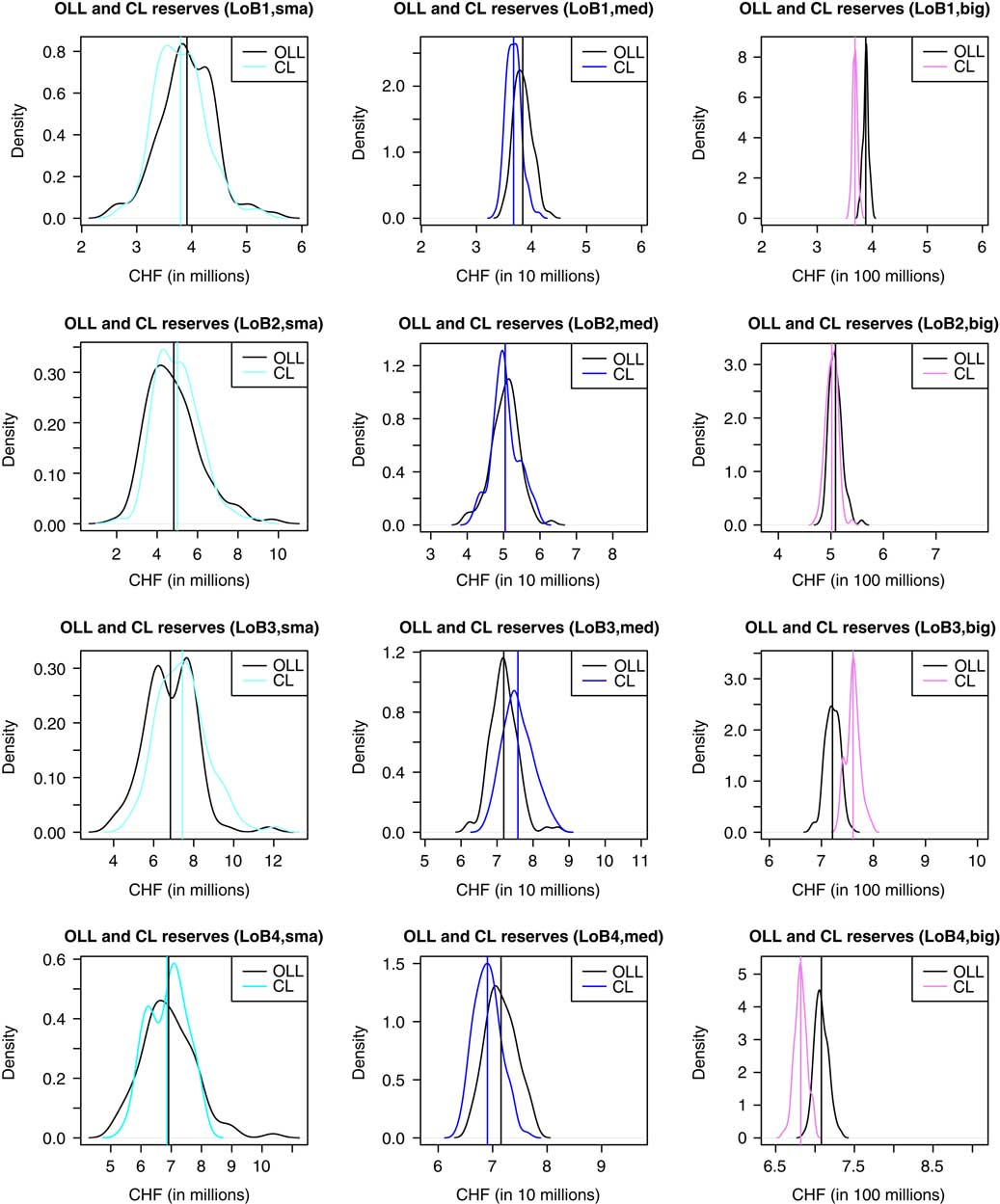
Figure 2 Densities of the OLL and the CL reserves for LoB1 (first row), LoB2 (second row), LoB3 (third row) and LoB4 (fourth row) of, respectively, the small company (left column), the medium company (middle column) and the big company (right column). The vertical lines indicate the corresponding sample means. OLL, outstanding loss liabilities; CL, chain-ladder; CHF, Swiss Franc.

Since the CL method works best for line of business LoB2, for the further analysis we will restrict to this line of business without any further reference. In particular, we define the tuple (k,v) $$\mathop{{\equals}}\limits^{{{\rm def}}} $$ (2, k, v), for all k=1, … , K and v ∈ {sma, med, big}. Moreover, V _v will refer to the volume of line of business LoB2, for all v ∈ {sma, med, big}.

For the sake of comparability of the different company sizes, we consider standardised OLL and CL reserves per unit of volume for the small, the medium and the big company. In Figure 3 (left), we look at

$$\left( {{{{\cal R}_{I}^{{(k,v)}} } \over {V_{v} }},{{\widehat{{\cal R}}_{I}^{{(k,v)}} } \over {V_{v} }}} \right)_{{1\leq k\leq K}} $$

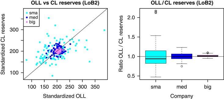
Figure 3 Scatterplot of the standardised OLL and the standardised CL reserves (per unit of volume) for the small (V _sma=25,000), the medium (V _med=250,000) and the big (V _big=2,500,000) company (left); the diagonal line corresponds to the identity line. Boxplots of the ratios of the OLL divided by the CL reserves for the small, the medium and the big company (right); the horizontal line indicates the reference value 1. OLL, outstanding loss liabilities; CL, chain-ladder; CHF, Swiss Franc.

for all v ∈ {sma, med, big}. This confirms the findings from above: due to the effect of the law of large numbers, the standard deviation of both the OLL and the CL reserves decreases with increasing volume V. For the small company, the CL reserves can be quite different from the OLL, whereas for the big company the CL reserves and the OLL are always rather close to each other.

We further investigate the observed differences between the OLL and the CL reserves in Figure 3 (right), where we consider the distributions of the ratios of the OLL divided by the CL reserves

$$\left( {{{{\cal R}_{I}^{{(k,v)}} } \over {\widehat{{\cal R}}_{I}^{{(k,v)}} }}} \right)_{{1\leq k\leq K}} $$

for all v ∈ {sma, med, big}. We get for k=1, … , K the ranges

$${{{\cal R}_{I}^{{(k,{\rm sma})}} } \over {\widehat{{\cal R}}_{I}^{{(k,{\rm sma})}} }}\,\in\,[0.47,2.17],\quad {{{\cal R}_{I}^{{(k,{\rm med})}} } \over {\widehat{{\cal R}}_{I}^{{(k,{\rm med})}} }}\,\in\,[0.75,\,1.23]\quad {\rm and}\quad {{{\cal R}_{I}^{{(k,{\rm big})}} } \over {\widehat{{\cal R}}_{I}^{{(k,{\rm big})}} }}\,\in\,[0.95,\,1.10].$$

Even though the CL method works fine on average for the small company, the OLL can be more than twice the CL reserves; or they can be only half of the CL reserves. With increasing volume V, these ratios get closer to 1. For the big portfolio the OLL are always within 10% of the CL reserves. Thus, with increasing volume V, we can be more and more confident about the precision of the CL reserves (supposed there is no bias involved). In the next section, we analyse whether this uncertainty can be captured by Mack’s CL uncertainty analysis.

2.2. Confidence intervals based on the mean-square errors of prediction

Since the CL reserves are only point predictors for the OLL, one should always consider the corresponding uncertainties. In Mack’s CL framework, this is done with the conditional MSEP. For the CL reserves $$\hat{{\cal R}}_{I} $$ at time I it is defined by

(5) $${\rm msep}_{{{\cal R}_{I} \,\mid\,{\cal D}_{I} }} \left( {\hat{{\cal R}}_{I} } \right){\equals}{\open E}\left[ {(\left. {{\cal R}_{I} {\minus}\hat{{\cal R}}_{I} } \right)^{2} \,\mid\,{\cal D}_{I} } \right]{\equals}{\rm Var}\left( {\left. {{\cal R}_{I} } \right|{\cal D}_{I} } \right){\plus}\left( {{\open E}\left[ {\left. {{\cal R}_{I} } \right|{\cal D}_{I} } \right]{\minus}\hat{{\cal R}}_{I} } \right)^{2} ,$$

see Mack (Reference Mack1993). The first summand on the right-hand side of equation (5) is called process variance and the second summand parameter estimation error. We define

$${\rm err}_{{{\cal R}_{I} \,\mid\,{\cal D}_{I} }} \left( {\hat{{\cal R}}_{I} } \right) {\equals} \left( {{\open E}\left[ {\left. {{\cal R}_{I} } \right|{\cal D}_{I} } \right]{\minus}\hat{{\cal R}}_{I} } \right)^{2} .$$

According to Theorem 3 and the subsequent corollary in Mack (Reference Mack1993), under Model Assumptions 1.1, $${\rm Var}({\cal R}_{I} \,\mid\,{\cal D}_{I} )$$ and $${\rm err}_{{{\cal R}_{I} \,\mid\,{\cal D}_{I} }} (\widehat{{\cal R}}_{I} )$$ can be estimated by

(6) $$\widehat{{{\rm Var}}}\left( {\left. {{\cal R}_{I} } \right|{\cal D}_{I} } \right) {\equals} \mathop{\sum}\limits_{i{\equals}I{\minus}J{\plus}1}^I \left( {\hat{C}_{{i,J\,\mid\,I}} } \right)^{2} \mathop{\sum}\limits_{j{\equals}I{\minus}i}^{J{\minus}1} {{\hat{\sigma }_{{j\,\mid\,I}}^{2} } \over {\left( {\hat{f}_{{j\,\mid\,I}} } \right)^{2} }}{1 \over {C_{{i,I{\minus}i}} \prod\limits_{j'{\equals}I{\minus}i}^{j{\minus}1} \hat{f}_{{j'\,\mid\,I}} }}$$

and

(7) $$\widehat{{{\rm err}}}_{{{\cal R}_{I} \,\mid\,{\cal D}_{I} }} \left( {\hat{{\cal R}}_{I} } \right) {\equals} \mathop{\sum}\limits_{i{\equals}I{\minus}J{\plus}1}^I \left( {\left( {\hat{C}_{{i,J\,\mid\,I}} } \right)^{2} {\plus}2\mathop{\sum}\limits_{m{\equals}i{\plus}1}^I \hat{C}_{{i,J\,\mid\,I}} \hat{C}_{{m,J\,\mid\,I}} } \right)\mathop{\sum}\limits_{j{\equals}I{\minus}i}^{J{\minus}1} {{\hat{\sigma }_{{j\,\mid\,I}}^{2} } \over {\left( {\hat{f}_{{j\,\mid\,I}} } \right)^{2} }}{1 \over {\mathop{\sum}\limits_{l{\equals}1}^{I{\minus}j{\minus}1} C_{{l,j}} }},$$

where we estimated the CL variance parameters $$\sigma _{j}^{2} $$ by

(8) $$\hat{\sigma }_{{j\,\mid\,I}}^{2} {\equals} {1 \over {I{\minus}j{\minus}2}}\mathop{\sum}\limits_{i{\equals}1}^{I{\minus}j{\minus}1} C_{{i,j}} \left( {{{C_{{i,j{\plus}1}} } \over {C_{{i,j}} }}{\minus}\hat{f}_{{j\,\mid\,I}} } \right)^{2}$$

for all j=0, … , J−2. Note that these are unbiased estimators for the CL variance parameters, see Mack (Reference Mack1993). The estimator $$\hat{\sigma }_{{J{\minus}1\,\mid\,I}}^{2} $$ for $$\sigma _{{J{\minus}1}}^{2} $$ can be calculated by extrapolating the usually exponentially decreasing series $$\hat{\sigma }_{{0\,\mid\,I}}^{2} ,\,\ldots\,,\hat{\sigma }_{{J{\minus}2\,\mid\,I}}^{2} $$ by one additional member by loglinear regression, see Mack (Reference Mack1993). Mack’s MSEP estimator is then given by

(9) $$\widehat{{{\rm msep}}}_{{{\cal R}_{I} \,\mid\,{\cal D}_{I} }} \left( {\hat{{\cal R}}_{I} } \right) {\equals} \widehat{{{\rm Var}}}\left( {\left. {{\cal R}_{I} } \right|{\cal D}_{I} } \right){\plus}\widehat{{{\rm err}}}_{{{\cal R}_{I} \,\mid\,{\cal D}_{I} }} \left( {\hat{{\cal R}}_{I} } \right).$$

For further analysis of the MSEP, we refer to sections 2.3 and 3, below. Now we check whether the OLL $${\cal R}_{I}^{{(k,v)}} $$ lie within the estimated confidence intervals given by

(10) $$\left( {\widehat{{\cal R}}_{I}^{{(k,v)}} {\minus}2\sqrt {\widehat{{{\rm msep}}}_{{{\cal R}_{I}^{{(k,v)}} \,\mid\,{\cal D}_{I} }} \left( {\widehat{{\cal R}}_{I}^{{(k,v)}} } \right)} ,\widehat{{\cal R}}_{I}^{{(k,v)}} {\plus}2\sqrt {\widehat{{{\rm msep}}}_{{{\cal R}_{I}^{{(k,v)}} \,\mid\,{\cal D}_{I} }} \left( {\widehat{{\cal R}}_{I}^{{(k,v)}} } \right)} } \right)$$

for k=1, … , K and v ∈ {sma, med, big}. See Figures 4–6 (left) for the results. We observe that the higher the volume V, the higher the percentage of the OLL that lie within the confidence intervals given by 11. For the small, respectively, the medium company we have that only 71% respectively, 72% of the OLL lie within the confidence intervals around the CL reserves. For the big company, the higher volume has a huge effect: 95% of the OLL lie within the confidence intervals around the CL reserves. This indicates that Mack’s MSEP formula may underestimate uncertainty if the volume V of the portfolio is too small (if confidence bounds of two standard deviations should cover roughly 95% of all observations).

Figure 4 Plot of the OLL and the CL reserves together with estimated confidence bounds of twice Mack’s MSEP around the CL reserves for the small company (left). Plot of the ratios of the OLL divided by the CL reserves together with estimated confidence bounds of twice Mack’s MSEP divided by the CL reserves around the value 1 for the small company (right); the horizontal line indicates the reference value 1. OLL, outstanding loss liabilities; CL, chain-ladder; MSEP, mean-square error of prediction; CHF, Swiss Franc.

Figure 5 Plot of the OLL and the CL reserves together with estimated confidence bounds of twice Mack’s MSEP around the CL reserves for the medium company (left). Plot of the ratios of the OLL divided by the CL reserves together with estimated confidence bounds of twice Mack’s MSEP divided by the CL reserves around the value 1 for the medium company (right); the horizontal line indicates the reference value 1. OLL, outstanding loss liabilities; CL, chain-ladder; MSEP, mean-square error of prediction; CHF, Swiss Franc.

Figure 6 Plot of the OLL and the CL reserves together with estimated confidence bounds of twice Mack’s MSEP around the CL reserves for the big company (left). Plot of the ratios of the OLL divided by the CL reserves together with estimated confidence bounds of twice Mack’s MSEP divided by the CL reserves around the value 1 for the big company (right); the horizontal line indicates the reference value 1. OLL, outstanding loss liabilities; CL, chain-ladder; MSEP, mean-square error of prediction.

We can draw the same conclusions from Figures 4–6 (right), where we divide the OLL by the CL reserves and check, for k=1, … , K and v ∈ {sma, med, big}, whether these ratios lie within the estimated confidence intervals given by

$$\left( {1{\minus}2{{\sqrt {\widehat{{{\rm msep}}}_{{{\cal R}_{I}^{{(k,v)}} \,\mid\,{\cal D}_{I} }} \left( {\widehat{{\cal R}}_{I}^{{(k,v)}} } \right)} } \over {\widehat{{\cal R}}_{I}^{{(k,v)}} }},1{\plus}2{{\sqrt {\widehat{{{\rm msep}}}_{{{\cal R}_{I}^{{(k,v)}} \,\mid\,{\cal D}_{I} }} \left( {\widehat{{\cal R}}_{I}^{{(k,v)}} } \right)} } \over {\widehat{{\cal R}}_{I}^{{(k,v)}} }}} \right)_{{1\leq k\leq K}}.$$

If we define

$$\alpha _{v} {\equals} {1 \over K}\mathop{\sum}\limits_{k{\equals}1}^K {{\sqrt {\widehat{{{\rm msep}}}_{{{\cal R}_{I}^{{(k,v)}} \,\mid\,{\cal D}_{I} }} \left( {\hat{{\cal R}}_{I}^{{(k,v)}} } \right)} } \over {\hat{{\cal R}}_{I}^{{(k,v)}} }}$$

for all v ∈ {sma, med, big}, we can interpret α _v as an average coefficient of variation of the CL reserves of company v. We observe the values

$$\alpha _{{{\rm sma}}} {\equals}14.0\,\%\,,\,\alpha _{{{\rm med}}} {\equals}5.5\,\%\,\,{\rm and}\,\alpha _{{{\rm big}}} {\equals} 3.2\,\%.$$

Thus, the coefficient of variation of the CL reserves is decreasing with increasing volume of the portfolio. This is in line with the findings of Table 4 in Bühlmann et al. (Reference Bühlmann, De Felice, Gisler, Moriconi and Wüthrich2009), where the authors analyse real car insurance data and where one observes a coefficient of variation of the CL reserves that ranges roughly between 2.5% and 28%, depending on the volume of the considered portfolio.

2.3. Mean-square error of prediction

We conclude section 2 by analysing the accuracy of the MSEP as defined in equation (5). We have

$${\open E}\left[ {{\rm msep}_{{{\cal R}_{I} \,\mid\,{\cal D}_{I} }} \left( {\widehat{{\cal R}}_{I} } \right)} \right]{\equals}{\open E}\left[ {\left( {{\cal R}_{I} {\minus}\widehat{{\cal R}}_{I} } \right)^{2} } \right].$$

If Mack’s MSEP estimator given in equation (9) is a “reasonable” estimator for the MSEP, then, due to the law of large numbers, we roughly expect

(11) $$\matrix{ {\beta _{v} }\!\!\!\!\!\hfill & {\mathop{{\equals}}\limits^{{{\rm def}}} {1 \over K}\mathop{\sum}\limits_{k{\equals}1}^K \widehat{{{\rm msep}}}_{{{\cal R}_{I}^{{(k,v)}} \,\mid\,{\cal D}_{I} }} \left( {\hat{{\cal R}}_{I}^{{(k,v)}} } \right) \,\approx\, {\open E}\left[ {{\rm msep}_{{{\cal R}_{I}^{{( \cdot ,v)}} \,\mid\,{\cal D}_{I} }} \left( {\hat{{\cal R}}_{I}^{{( \cdot ,v)}} } \right)} \right]} \hfill \cr \hfill & {{\equals}{\open E}\left[ {\left( {{\cal R}_{I}^{{( \cdot ,v)}} {\minus}\hat{{\cal R}}_{I}^{{( \cdot ,v)}} } \right)^{2} } \right]\,\approx\,{1 \over K}\mathop{\sum}\limits_{k{\equals}1}^K \left( {{\cal R}_{I}^{{(k,v)}} {\minus}\hat{{\cal R}}_{I}^{{(k,v)}} } \right)^{2} \mathop{{\equals}}\limits^{{{\rm def}}} \gamma _{v} } \hfill \cr } $$

for all three companies v ∈ {sma, med, big}. For the square roots of the ratios γ _v /β _v , we get

$$\sqrt {{{\gamma _{{{\rm sma}}} } \over {\beta _{{{\rm sma}}} }}} {\equals} 1.87,\,\sqrt {{{\gamma _{{{\rm med}}} } \over {\beta _{{{\rm med}}} }}} {\equals}1.67\,{\rm and}\,\sqrt {{{\gamma _{{{\rm big}}} } \over {\beta _{{{\rm big}}} }}} {\equals}0.96.$$

Due to equation (11), these values are expected to be roughly equal to 1. For the small and the medium company, the square roots of the average Mack’s MSEPs are too small, i.e. we underestimate the true MSEP in both cases. This explains why for these two companies many OLL (29% respectively 28%) lie outside the confidence intervals given in (10). For the big company, Mack’s MSEP seems to be of appropriate size.

3.1. Distributional plots

In Mack’s CL model, the process variance and the parameter estimation error are estimated by equations (6) and (7), respectively. In order to be able to compare the different companies, we consider standardised versions of these estimators, dividing by the CL reserves. In Figure 7, we consider the distributions of

$$\left( {{{\sqrt {\widehat{{{\rm Var}}}\left( {\left. {{\cal R}_{I}^{{(k,v)}} } \right|{\cal D}_{I} } \right)} } \over {\hat{{\cal R}}_{I}^{{(k,v)}} }}} \right)_{{1\leq k\leq K}} \,{\rm and}\,\left( {{{\sqrt {\widehat{{{\rm err}}}_{{{\cal R}_{I}^{{(k,v)}} \,\mid\,{\cal D}_{I} }} \left( {\hat{{\cal R}}_{I}^{{(k,v)}} } \right)} } \over {\hat{{\cal R}}_{I}^{{(k,v)}} }}} \right)_{{1\leq k\leq K}}$$

for all v ∈ {sma, med, big}. Due to the law of large numbers, the square-rooted standardised process variance and the square-rooted standardised parameter estimation error decrease in the volume V, as well as the support, becoming more narrow with increasing V.

Figure 7 Boxplots of the square-rooted standardised process variances (left) and the square-rooted standardised parameter estimation errors (right) for the small, the medium and the big company.

Interestingly, the proportion of the process variance to the MSEP is increasing in the volume V. We can observe this in Figure 8, where we look at the distributions of

$$\left( {{{\widehat{{{\rm Var}}}\left( {\left. {{\cal R}_{I}^{{(k,v)}} } \right|{\cal D}_{I} } \right)} \over {\widehat{{{\rm msep}}}_{{{\cal R}_{I}^{{(k,v)}} \,\mid\,{\cal D}_{I} }} \left( {\hat{{\cal R}}_{I}^{{(k,v)}} } \right)}}} \right)_{{1\leq k\leq K}} \,{\rm and}\,\left( {\sqrt {{{\widehat{{{\rm Var}}}\left( {\left. {{\cal R}_{I}^{{(k,v)}} } \right|{\cal D}_{I} } \right)} \over {\widehat{{{\rm err}}}_{{{\cal R}_{I}^{{(k,v)}} \,\mid\,{\cal D}_{I} }} \left( {\hat{{\cal R}}_{I}^{{(k,v)}} } \right)}}} } \right)_{{1\leq k\leq K}} $$

for all v ∈ {sma, med, big}. If we define

$$\delta _{v} {\equals} {1 \over K}\mathop{\sum}\limits_{k{\equals}1}^K {{\widehat{{{\rm Var}}}\left( {\left. {{\cal R}_{I}^{{(k,v)}} } \right|{\cal D}_{I} } \right)} \over {\widehat{{{\rm msep}}}_{{{\cal R}_{I}^{{(k,v)}} \,\mid\,{\cal D}_{I} }} \left( {\hat{{\cal R}}_{I}^{{(k,v)}} } \right)}}\,{\rm and}\,{\varepsilon}_{v} {\equals} {1 \over K}\mathop{\sum}\limits_{k{\equals}1}^K \sqrt {{{\widehat{{{\rm Var}}}\left( {\left. {{\cal R}_{I}^{{(k,v)}} } \right|{\cal D}_{I} } \right)} \over {\widehat{{{\rm err}}}_{{{\cal R}_{I}^{{(k,v)}} \,\mid\,{\cal D}_{I} }} \left( {\hat{{\cal R}}_{I}^{{(k,v)}} } \right)}}} $$

to be the corresponding sample means, for all v ∈ {sma, med, big}, we get the values

$$\delta _{{{\rm sma}}} {\equals}65\,\%\,,\quad \delta _{{{\rm med}}} {\equals}68\,\%\,\quad {\rm and}\quad \delta _{{{\rm big}}} {\equals}83\,\%$$

as well as

$${\varepsilon}_{{{\rm sma}}} {\equals}1.4,\quad {\varepsilon}_{{{\rm med}}} {\equals}1.5\quad {\rm and}\quad {\varepsilon}_{{{\rm big}}} {\equals}2.2.$$

Figure 8 Boxplots of the ratios of the process variances divided by the MSEPs for the small, the medium and the big company (left); the horizontal line indicates the value 50%. Boxplots of the ratios of the square-rooted process variances divided by the square-rooted parameter estimation errors for the small, the medium and the big company (right); the horizontal line indicates the value 1. MSEP, mean-square error of prediction.

We conclude that the importance of the parameter estimation error is decreasing in the volume V and the process variance becomes the dominant term of the MSEP for bigger companies. The increase of the average proportion of the process variance to the MSEP is moderate in going from the small company to the medium company (from 65% to 68%) and rather large in going from the medium company to the big company (from 68% to 83%). For the small and the medium company, the square-rooted process variance is roughly 50% higher than the square-rooted parameter estimation error, on average. For the big company, the square-rooted process variance is more than twice the square-rooted parameter estimation error, on average.

3.2. Process variance

We take a closer look at the process variance. If Mack’s estimator $$\widehat{{{\rm Var}}}({\cal R}_{I} \,\mid\,{\cal D}_{I} )$$ for the process variance given in equation (6) is “reasonable”, then, due to the law of large numbers, we roughly expect

(12) $$\zeta _{v} \mathop{{\equals}}\limits^{{{\rm def}}} {1 \over K}\mathop{\sum}\limits_{k{\equals}1}^K \widehat{{{\rm Var}}}\left( {\left. {{\cal R}_{I}^{{(k,v)}} } \right|{\cal D}_{I} } \right) \,\approx\, {\open E}\left[ {{\rm Var}\left( {\left. {{\cal R}_{I}^{{( \cdot ,v)}} } \right|{\cal D}_{I} } \right)} \right]$$

for all companies v ∈ {sma, med, big}. In order to analyse the accuracy of Mack’s estimator for the process variance, we approximate the conditional variance on the right-hand side of equation (12) using the variance decomposition formula and equation (1). Indeed, we can write

$$\eqalignno{ {\rm Var}\left( {{\cal R}_{I} } \right) {\equals} {\rm Var}\left( {{\open E}\left[ {\left. {{\cal R}_{I} } \right|{\cal D}_{I} } \right]} \right){\plus}{\open E}\left[ {{\rm Var}\left( {\left. {{\cal R}_{I} } \right|{\cal D}_{I} } \right)} \right] \cr {\equals} {\rm Var}\left( {\mathop{\sum}\limits_{i{\equals}I{\minus}J{\plus}1}^I C_{{i,I{\minus}i}} \left( {\prod\limits_{j{\equals}I{\minus}i}^{J{\minus}1} f_{j} {\minus}1} \right)} \right){\plus}{\open E}\left[ {{\rm Var}({\cal R}_{I} \,\mid\,{\cal D}_{I} )} \right].$$

Using the assumption of independence of the accident years, this leads to

$${\open E}\left[ {{\rm Var}({\cal R}_{I} \,\mid\,{\cal D}_{I} )} \right] {\equals} {\rm Var}\left( {{\cal R}_{I} } \right){\minus}\mathop{\sum}\limits_{i{\equals}I{\minus}J{\plus}1}^I {\rm Var}\left( {C_{{i,I{\minus}i}} } \right)\left( {\prod\limits_{j{\equals}I{\minus}i}^{J{\minus}1} f_{j} {\minus}1} \right)^{2}$$

We can use sample variances to estimate $${\rm Var}({\cal R}_{I} )$$ and Var (C _i,I−i ), for all i=I−J+1, … , I. Moreover, in view of equation (2) we can estimate the CL factor f _j by the global estimate

(13) $$\bar{f}_{{j,v}} {\equals} {1 \over K}\mathop{\sum}\limits_{k{\equals}1}^K {{\mathop{\sum}\limits_{i{\equals}1}^I C_{{i,j{\plus}1}}^{{(k,v)}} } \over {\mathop{\sum}\limits_{i{\equals}1}^I C_{{i,j}}^{{(k,v)}} }}$$

for all j=0, … , J−1, depending on the considered company v ∈ {sma, med, big}. We remark that the global estimates $\bar{f}_{{0,v}} $ , … , $\bar{f}_{{J{\minus}1,v}} $ of the CL factors f ₀, … , f _J−1 consider the full developments of the cumulative claims payments in all accident years i=1, … , I. They can only be calculated since for all upper claims reserving triangles we also know the corresponding lower triangles. Starting from equation (12), we roughly expect

$$\matrix{ {\zeta _{v} } \hfill \!\!\!\!\!{\approx\, {\open E}\left[ {{\rm Var}\left( {\left. {{\cal R}_{I}^{{( \cdot ,v)}} } \right|{\cal D}_{I} } \right)} \right]} {\,\approx\, {1 \over {K{\minus}1}}\mathop{\sum}\limits_{k{\equals}1}^K \left( {{\cal R}_{I}^{{(k,v)}} {\minus}{1 \over K}\mathop{\sum}\limits_{l{\equals}1}^K {\cal R}_{I}^{{(l,v)}} } \right)^{2} } \hfill \cr {} \hfill & {{\minus}\mathop{\sum}\limits_{i{\equals}I{\minus}J{\plus}1}^I {1 \over {K{\minus}1}}\mathop{\sum}\limits_{k{\equals}1}^K \left( {C_{{i,I{\minus}i}}^{{(k,v)}} {\minus}{1 \over K}\mathop{\sum}\limits_{l{\equals}1}^K C_{{i,I{\minus}i}}^{{(l,v)}} } \right)^{2} \left( {\prod\limits_{j{\equals}I{\minus}i}^{J{\minus}1} \bar{f}_{{j,v}} {\minus}1} \right)^{2} \mathop{{\equals}}\limits^{{{\rm def}}} \eta _{v} } \hfill \cr } $$

For the square roots of the ratios η _v /ζ _v we get

$$\sqrt {{{\eta _{{{\rm sma}}} } \over {\zeta _{{{\rm sma}}} }}} {\equals}2.21,\,\sqrt {{{\eta _{{{\rm med}}} } \over {\zeta _{{{\rm med}}} }}} {\equals}1.65\,{\rm and}\,\sqrt {{{\eta _{{{\rm big}}} } \over {\zeta _{{{\rm big}}} }}} {\equals}0.81$$

We may conclude that we underestimate the process variance for small volumes V of the portfolio and overestimate it for big volumes V.

3.3. Parameter estimation error

We analyse Mack’s estimator for the parameter estimation error given in equation (7) in two different ways. To this end, for both methods we define

$$\theta _{{k,v}} {\equals} {{\sqrt {\widehat{{{\rm err}}}_{{{\cal R}_{I}^{{(k,v)}} \,\mid\,{\cal D}_{I} }} \left( {\hat{{\cal R}}_{I}^{{(k,v)}} } \right)} } \over {\hat{{\cal R}}_{I}^{{(k,v)}} }}$$

to be the proportions of the square-rooted Mack’s estimates of the parameter estimation error to the CL reserves, for all k=1, … , K and v ∈ {sma, med, big}.

For the first method, we note that we have

$${\rm err}_{{{\cal R}_{I} \,\mid\,{\cal D}_{I} }} \left( {\hat{{\cal R}}_{I} } \right) {\equals} \left( {\mathop{\sum}\limits_{i{\equals}I{\minus}J{\plus}1}^I C_{{i,I{\minus}i}} \left( {\prod\limits_{j{\equals}I{\minus}i}^{J{\minus}1} f_{j} {\minus}\prod\limits_{j{\equals}I{\minus}i}^{J{\minus}1} \hat{f}_{{j\,\mid\,I}} } \right)} \right)^{2}$$

see Mack (Reference Mack1993). If Mack’s estimator for the parameter estimation error given in equation (7) is a “reasonable” estimator, then, we roughly expect

$$\bar{\theta }_{v} \mathop{{\equals}}\limits^{{{\rm def}}} {1 \over K}\mathop{\sum}\limits_{k{\equals}1}^K \theta _{{k,v}} \,\approx\,{1 \over K}\mathop{\sum}\limits_{k{\equals}1}^K {{\left| {\mathop{\sum}\limits_{i{\equals}I{\minus}J{\plus}1}^I C_{{i,I{\minus}i}}^{{(k,v)}} \left( {\prod\limits_{j{\equals}I{\minus}i}^{J{\minus}1} \bar{f}_{{j,v}} {\minus}\prod\limits_{j{\equals}I{\minus}i}^{J{\minus}1} \hat{f}_{{j\,\mid\,I}}^{{(k,v)}} } \right)} \right|} \over {\hat{{\cal R}}_{I}^{{(k,v)}} }}\mathop{{\equals}}\limits^{{{\rm def}}} \bar{\vartheta }_{v}$$

for all v ∈ {sma, med, big}. For the ratios ϑ _v /θ _v we get

(14) $${{\bar{\vartheta }_{{{\rm sma}}} } \over {\bar{\theta }_{{{\rm sma}}} }}{\equals}1.74,\quad {{\bar{\vartheta }_{{{\rm med}}} } \over {\bar{\theta }_{{{\rm med}}} }}{\equals}1.72\quad {\rm and}\quad {{\bar{\vartheta }_{{{\rm big}}} } \over {\bar{\theta }_{{{\rm big}}} }}{\equals}1.44.$$

For all three companies, using Mack’s estimator given in equation (7), we seem to underestimate the parameter estimation error. For the big company, however, the situation gets slightly better.

The second method to analyse Mack’s estimator for the parameter estimation error is based on a bootstrap argument. In England and Verrall (Reference England and Verrall2006), the authors use a bootstrap technique in order to simulate arbitrarily many upper triangles based on a given upper claims reserving triangle. These bootstrapped upper triangles can then be used to estimate the parameter estimation error. Since we are already provided with K simulated upper claims reserving triangles coming from the same underlying distribution, we do not need to apply a bootstrap, but we can directly estimate the parameter estimation error using the K upper triangles.

For all three companies v ∈ {sma, med, big}, we order the K simulations according to the CL reserves and write

$$\hat{{\cal R}}_{I}^{{((1),v)}} \,\lt\,\hat{{\cal R}}_{I}^{{((2),v)}} \,\lt\, \cdots \,\lt\,\hat{{\cal R}}_{I}^{{((K),v)}} $$

for the ordered CL reserves. We use the same ordering (κ)_1≤κ≤K also for the estimates θ _(⋅),v and for the entries $$C_{{i,I{\minus}i}}^{{(( \cdot ),v)}} $$ on the diagonals of the triangles, for all v ∈ {sma, med, big} and i=1, … , I. We define the bootstrap-like estimates

(15) $$\lambda _{{(\kappa ),k,v}} {\equals}{{\left| {\mathop{\sum}\limits_{i{\equals}I{\minus}J{\plus}1}^I C_{{i,I{\minus}i}}^{{((\kappa ),v)}} \left( {\prod\limits_{j{\equals}I{\minus}i}^{J{\minus}1} \bar{f}_{{j,v}} {\minus}\prod\limits_{j{\equals}I{\minus}i}^{J{\minus}1} \hat{f}_{{j\,\mid\,I}}^{{(k,v)}} } \right)} \right|} \over {\hat{{\cal R}}_{I}^{{((\kappa ),v)}} }}$$

of the (relative) parameter estimation errors, and the corresponding sample means

$$\bar{\lambda }_{{(\kappa ),v}} {\equals} {1 \over K}\mathop{\sum}\limits_{k{\equals}1}^K \lambda _{{(\kappa ),k,v}}$$

for all κ=1, … , K, k=1, … , K and v ∈ {sma, med, big}. Note that for the bootstrap-like estimates (λ _(κ),k,v )_1≤k≤K given in equation (15), we fix the last known diagonal of the upper claims reserving triangle of the κth ordered simulation and vary only the estimated CL factors. For every 1≤κ≤K, this leads to K estimates of the parameter estimation error.

First, we focus on three specific simulations. We consider the simulation with the lowest CL reserves (κ=1), the simulation with the median CL reserves (κ=50) and the simulation with the highest CL reserves (κ=100). In Figure 9, we provide the distributions of the bootstrap-like estimates (λ _(κ),k,v )_1≤k≤K , together with the corresponding sample means $$\bar{\lambda }_{{(k),v}} $$ , and Mack’s estimates θ _(κ),v as reference values, for κ=150,100 and v ∈ {sma, med, big}. For the small company, Mack’s estimate θ _(κ),v is clearly smaller than the mean $$\bar{\lambda }_{{(k),v}} $$ of the bootstrap-like estimates for the simulation with the lowest CL reserves (κ=1) and close to $$\bar{\lambda }_{{(k),v}} $$ for the simulations with the median (κ=50) and the highest CL reserves (κ=100). For the medium company, we have that the higher the CL reserves, the closer Mack’s estimate θ _(κ),v gets to the mean $$\bar{\lambda }_{{(k),v}} $$ of the bootstrap-like estimates. For the big company, we cannot see much difference between the three simulations: Mack’s estimate θ _(κ),v is always smaller than the mean $$\bar{\lambda }_{{(k),v}} $$ of the bootstrap-like estimates.

Figure 9 Densities of the bootstrap-like estimates λ _(κ),k,v of the parameter estimation error together with Mack’s estimates θ _(κ),v (vertical solid lines) for the simulation with the lowest CL reserves (left column), the median CL reserves (middle column) and the highest CL reserves (right column) resp. the small company (top row), the medium company (middle row) and the big company (bottom row). The vertical dotted black lines indicate the sample means $$\bar{\lambda }_{{(k),v}} $$ of the bootstrap-like estimates.

Since the CL reserves are ordered in increasing manner according to κ, we have that the bigger κ, the bigger the denominator in equation (15). Therefore, the densities of the bootstrap-like estimates (λ _(κ),k,v )_1≤k≤K get more narrow with increasing κ. This effect gets smaller for increasing volume V, since the CL reserves get less widely spread, due to the law of large numbers.

We remark that the observations regarding Figure 9 are rather sensitive to the choice of κ. That is, choosing a different small, medium or large κ, we get different results. Therefore, for all companies v ∈ {sma, med, big}, we analyse whether we see some trend in the relation between Mack’s estimates θ _(κ),v and the means $$\bar{\lambda }_{{(k),v}} $$ of the bootstrap-like estimates for increasing CL reserves $$\widehat{{\cal R}}_{I}^{{((\kappa ),v)}} $$ . To this end, in view of equation (14), we define the ratios

$$\mu _{{(\kappa ),v}} {\equals} {{\bar{\lambda }_{{(\kappa ),v}} } \over {\theta _{{(\kappa ),v}} }}$$

for all κ=1, … , K and v ∈ {sma, med, big}. In Figure 10, we then consider

$$\left( {{{\hat{{\cal R}}_{I}^{{((\kappa ),v)}} } \over {V_{v} }},\mu _{{(\kappa ),v}} } \right)_{{1\leq \kappa \leq K}}.$$

Figure 10 Scatterplots of the standardised CL reserves and the ratios of the means of the bootstrap-like estimates of the parameter estimation error to Mack’s estimates for the small company (left), the medium company (middle) and the big company (right). The horizontal black lines indicate the reference value 1. The red lines indicate the linear regression line.

We also provide the corresponding regression lines resulting from a linear regression analysis with the standardised CL reserves as independent variable and the ratios of the two estimates of the parameter estimation error as dependent variable, using ordinary least squares to minimise the residuals. For all three companies, we observe a bias: Mack’s estimates θ _(κ),v tend to be too small compared to the means $$\bar{\lambda }_{{(k),v}} $$ of the bootstrap-like estimates, leading to an underestimation of the parameter estimation error when using Mack’s estimator. This bias is smallest for the big company, see also equation (14). Moreover, for the small and the medium company, we observe a tendency that the ratios of the means of the bootstrap-like estimates of the parameter estimation error to Mack’s estimates get closer to the reference value 1 with increasing CL reserves. For the big company, these ratios seem to not depend on the CL reserves.

Combining these observations, we may deduce, on the one hand, that Mack’s estimator for the parameter estimation error in case of a small or a medium portfolio works slightly better for claims reserving data with corresponding CL reserves that are rather high, relative to the underlying distribution. On the other hand, Mack’s estimator for the parameter estimation error seems to work equally well in case of a big portfolio, independently of the size of the CL reserves.

4.1. Analysis of the claims development results

For t+1=I+1, … , I+J, we define the CDR in accounting year t+1 by

(16) $${\rm CDR}_{{t{\plus}1}} {\equals}\mathop{\sum}\limits_{i{\equals}t{\minus}J{\plus}1}^I {\open E}\left[ {C_{{i,J}} \,\mid\,{\cal D}_{t} } \right]{\minus}{\open E}\left[ {C_{{i,J}} \,\mid\,{\cal D}_{{t{\plus}1}} } \right].$$

The CDR in accounting year t+1 reflects the change in the prediction of the ultimate claims when the new information of accounting year t+1 is available. A positive CDR corresponds to a gain in the sense that the estimates of the ultimate claims are lower at time t+1 than at time t. A negative CDR corresponds to a loss. On average, we do neither expect a gain nor a loss if the model is correct: indeed, due to the tower property of conditional expectation, see Williams (Reference Williams1991), from equation (16) we immediately get, for all t+1=I+1, … , I+J,

$${\open E}\left[ {{\rm CDR}_{{t{\plus}1}} \,\mid\,{\cal D}_{t} } \right] {\equals} 0.$$

Within the CL framework, a natural estimator for CDR _t+1 is

$$\widehat{{{\rm CDR}}}_{{t{\plus}1}} {\equals} \mathop{\sum}\limits_{i{\equals}t{\minus}J{\plus}1}^I \hat{C}_{{i,J\,\mid\,t}} {\minus}\hat{C}_{{i,J\,\mid\,t{\plus}1}} {\equals} \hat{{\cal R}}_{t} {\minus}\left( {\hat{{\cal R}}_{{t{\plus}1}} {\plus}\mathop{\sum}\limits_{i{\equals}t{\minus}J{\plus}1}^I C_{{i,t{\minus}i{\plus}1}} {\minus}C_{{i,t{\minus}i}} } \right)$$

for all t+1=I+1, … , I+J. Thus, the estimated CDR in accounting year t+1 can be expressed as the difference between the CL reserves at time t and the sum of the CL reserves at time t+1 and the payments in accounting year t+1. We remark that, in practice, at the end of accounting year I, $$\widehat{{{\rm CDR}}}_{{t{\plus}1}} $$ cannot be calculated for t+1≥I+1, as one only has information up to accounting year I and, hence, the reserves at time t+1 and the payments in accounting year t+1 are unknown for t+1≥I+1. However, in our CL analysis (using the synthetic data), we are provided with upper claims reserving triangles for which we also know the corresponding lower triangles. Therefore, we can calculate $$\widehat{{{\rm CDR}}}_{{t{\plus}1}} $$ for accounting years t+1=I+1, … , I+J.

For reasons of comparability, we are more interested in a CDR relative to the reserves at time I. We define

$${\rm CDR}_{{{\rm rel},t{\plus}1}} {\equals} {{{\rm CDR}_{{t{\plus}1}} } \over {\mathop{\sum}\limits_{i{\equals}I{\minus}J{\plus}1}^I {\open E}\left[ {C_{{i,J}} \,\mid\,{\cal D}_{I} } \right]{\minus}C_{{i,I{\minus}i}} }}$$

for all t+1=I+1, … , I+J. Using the tower property of conditional expectation, see Williams (Reference Williams1991), we also get for the relative CDR

(17) $${\open E}\left[ {{\rm CDR}_{{{\rm rel},t{\plus}1}} \,\mid\,{\cal D}_{t} } \right]{\equals}0$$

for all t+1=I+1, … , I+J. The CL estimator $$\widehat{{{\rm CDR}}}_{{{\rm rel},t{\plus}1}} $$ for CDR_rel,t+1, for t+1=I+1, … , I+J, is then given by

$$\widehat{{{\rm CDR}}}_{{{\rm rel},t{\plus}1}} {\equals} {{\widehat{{{\rm CDR}}}_{{t{\plus}1}} } \over {\hat{{\cal R}}_{I} }}.$$

The information $${\cal D}_{I} $$ at the end of accounting year I only allows us to estimate the uncertainties of the CDRs. For CDR _t+1, for t+1=I+1, … , I+J, the MSEP with respect to $${\cal D}_{I} $$ is defined by

$${\rm msep}_{{{\rm CDR}_{{t{\plus}1}} \,\mid\,{\cal D}_{I} }} \left( 0 \right) {\equals} {\open E}\left[ {\left. {\left( {{\rm CDR}_{{t{\plus}1}} {\minus}0} \right)^{2} } \right|{\cal D}_{I} } \right].$$

As estimators for the MSEPs, we can use the formulas given in Wüthrich and Merz (Reference Wüthrich and Merz2015). For t+1=I+1, we have the Merz–Wüthrich formula, see (2.28) in Wüthrich and Merz (Reference Wüthrich and Merz2015),

$$\eqalignno{ \widehat{{{\rm msep}}}_{{{\rm CDR}_{{I{\plus}1}} \,\mid\,{\cal D}_{I} }} \left( 0 \right){\equals} \mathop{\sum}\limits_{i{\equals}I{\minus}J{\plus}1}^I \left( {\hat{C}_{{i,J\,\mid\,I}} } \right)^{2} {{\hat{\sigma }_{{I{\minus}i\,\mid\,I}}^{2} } \over {\left( {\hat{f}_{{I{\minus}i\,\mid\,I}} } \right)^{2} }}{1 \over {C_{{i,I{\minus}i}} }}{\plus}\left( {\left( {\hat{C}_{{i,J\,\mid\,I}} } \right)^{2} {\plus}2\mathop{\sum}\limits_{m{\equals}i{\plus}1}^I \hat{C}_{{i,J\,\mid\,I}} \hat{C}_{{m,J\,\mid\,I}} } \right) \cr {\times}\left( {{{\hat{\sigma }_{{I{\minus}i\,\mid\,I}}^{2} } \over {\left( {\hat{f}_{{I{\minus}i\,\mid\,I}} } \right)^{2} }}{1 \over {\mathop{\sum}\limits_{l{\equals}1}^{i{\minus}1} C_{{l,I{\minus}i}} }}{\plus}\mathop{\sum}\limits_{j{\equals}I{\minus}i{\plus}1}^{J{\minus}1} {{C_{{I{\minus}j,j}} } \over {\mathop{\sum}\limits_{l{\equals}1}^{I{\minus}j} C_{{l,j}} }}{{\hat{\sigma }_{{j\,\mid\,I}}^{2} } \over {\left( {\hat{f}_{{j\,\mid\,I}} } \right)^{2} }}{1 \over {\mathop{\sum}\limits_{l{\equals}1}^{I{\minus}j{\minus}1} C_{{l,j}} }}} \right).$$

Due to the tower property of conditional expectation, see Williams (Reference Williams1991), for t+1=I+2, … , I+J we have

$${\rm msep}_{{{\rm CDR}_{{t{\plus}1}} \,\mid\,{\cal D}_{I} }} \left( 0 \right) {\equals} {\open E}\left[ {\left. {{\open E}\left[ {\left. {\left( {{\rm CDR}_{{t{\plus}1}} {\minus}0} \right)^{2} } \right|{\cal D}_{t} } \right]} \right|{\cal D}_{I} } \right] {\equals} {\open E}\left[ {\left. {{\rm msep}_{{{\rm CDR}_{{t{\plus}1}} \,\mid\,{\cal D}_{t} }} \left( 0 \right)} \right|{\cal D}_{I} } \right],$$

which leads to the estimators, see (2.36) in Wüthrich and Merz (Reference Wüthrich and Merz2015),

$$\eqalignno{ & \widehat{{{\rm msep}}}_{{{\rm CDR}_{{t{\plus}1}} \,\mid\,{\cal D}_{I} }} \left( 0 \right) \mathop{{\equals}}\limits^{{{\rm def}}} \hat{{\open E}}\left[ {\left. {\widehat{{{\rm msep}}}_{{{\rm CDR}_{{t{\plus}1}} \,\mid\,{\cal D}_{t} }} \left( 0 \right)} \right|{\cal D}_{I} } \right] \cr & \mathop{{\equals}}\limits^{{{\rm def}}} \mathop{\sum}\limits_{i{\equals}t{\minus}J{\plus}1}^I \left( {\hat{C}_{{i,J\,\mid\,I}} } \right)^{2} {{\hat{\sigma }_{{t{\minus}i\,\mid\,I}}^{2} } \over {\left( {\hat{f}_{{t{\minus}i\,\mid\,I}} } \right)^{2} }}{1 \over {C_{{i,I{\minus}i}} \prod\limits_{j{\equals}I{\minus}i}^{t{\minus}i{\minus}1} \hat{f}_{{j\,\mid\,I}} }}{\plus}\left( {\left( {\widehat{C}_{{i,J\,\mid\,I}} } \right)^{2} {\plus}2\mathop{\sum}\limits_{m{\equals}i{\plus}1}^I \hat{C}_{{i,J\,\mid\,I}} \hat{C}_{{m,J\,\mid\,I}} } \right) \cr & \quad{\times}\left( {{{\hat{\sigma }_{{t{\minus}i\,\mid\,I}}^{2} } \over {\left( {\hat{f}_{{t{\minus}i\,\mid\,I}} } \right)^{2} }}{1 \over {\mathop{\sum}\limits_{l{\equals}1}^{I{\minus}1{\minus}(t{\minus}i)} C_{{l,t{\minus}i}} }}\prod\limits_{r{\equals}1}^{t{\minus}I} \left( {1{\minus}{{C_{{i{\minus}r,I{\minus}(i{\minus}r)}} } \over {\mathop{\sum}\limits_{l{\equals}1}^{i{\minus}r} C_{{l,I{\minus}(i{\minus}r)}} }}} \right)} \right. \cr & \quad{\plus}\left. {\mathop{\sum}\limits_{j{\equals}t{\minus}i{\plus}1}^{J{\minus}1} {{\widehat{\sigma }_{{j\,\mid\,I}}^{2} } \over {\left( {\hat{f}_{{j\,\mid\,I}} } \right)^{2} }}{1 \over {\mathop{\sum}\limits_{l{\equals}1}^{I{\minus}j{\minus}1} C_{{l,j}} }}{{C_{{t{\minus}j,I{\minus}(t{\minus}j)}} } \over {\mathop{\sum}\limits_{l{\equals}1}^{t{\minus}j} C_{{l,I{\minus}(t{\minus}j)}} }}\prod\limits_{r{\equals}0}^{t{\minus}I{\minus}1} \left( {1{\minus}{{C_{{I{\minus}(j{\minus}r),j{\minus}r}} } \over {\mathop{\sum}\limits_{l{\equals}1}^{I{\minus}(j{\minus}r)} C_{{l,j{\minus}r}} }}} \right)} \right).$$

In order for the MSEPs to be on the same scale as the relative CDRs, we standardise the MSEPs by dividing through the CL reserves at time t=I and define

$$\psi _{{t{\plus}1,v}} {\equals} {1 \over K}\mathop{\sum}\limits_{k{\equals}1}^K {{\sqrt {\widehat{{{\rm msep}}}_{{{\rm CDR}_{{t{\plus}1}}^{{(k,v)}} \,\mid\,{\cal D}_{I} }} \left( 0 \right)} } \over {\hat{{\cal R}}_{I}^{{(k,v)}} }}$$

to be the average relative MSEPs of the CDRs, for all accounting years t+1=I+1, … , I+J and companies v ∈ {sma, med, big}. In Figure 11, we consider the distributions of the estimated relative CDRs

$$\left( {\widehat{{{\rm CDR}}}_{{{\rm rel},t{\plus}1}}^{{(k,v)}} } \right)_{{1\leq k\leq K}}$$

together with the average estimated confidence intervals

$$\left( {{\minus}2\psi _{{t{\plus}1,v}} ,2\psi _{{t{\plus}1,v}} } \right)$$

for all accounting years t+1=I+1, … , I+J and v ∈ {sma, med, big}. For the estimated relative CDR in accounting year t+1=I+1 we get

$$\widehat{{{\rm CDR}}}_{{{\rm rel},I{\plus}1}}^{{(k,v)}} \in \left\{ {\matrix{ {[{\minus}53.6\%\,,28.6\%\,],} \hfill & {{\rm if\ \it v{\equals}\rm sma,}}\hfill\cr{[{\minus}15.2\%\,,9.2\%\,],} \hfill & {{\rm if\ \it v{\equals}\rm med,}}\hfill\cr{[{\minus}6.3\%\,,{\minus}0.7\%\,],} \hfill & {{\rm if\ \it v{\equals}\rm big,}} \hfill \cr } } \right.$$

for all k=1, … , K. In particular, the distribution of the estimated relative CDR in accounting year t+1=I+1 gets more narrow with increasing volume V, due to the law of large numbers. In view of equation (17), we roughly expect the estimated relative CDRs to be distributed around 0. For the small and the medium company, we can observe positive and negative CDRs in accounting year t+1=I+1. In the worst-case scenario of the small company, the sum of the payments in accounting year t+1=I+1 and the CL reserves at time I+1 is roughly 50% bigger than the CL reserves at time I, corresponding to a huge loss. For the big company, the estimated relative CDRs in accounting year t+1=I+1 are always negative, but they stay within only −6.3% of the reserves at time I. For all three companies, the confidence intervals of twice the average relative MSEP ψ _I+1,v around 0 seem to be of appropriate size for the estimated relative CDRs in accounting year t+1=I+1.

Figure 11 Boxplots of the estimated relative CDRs $$\widehat{{{\rm CDR}}}_{{{\rm rel},t{\plus}1}}^{{(k,v)}} $$ in accounting years t+1=I+1, …, I+J together with confidence bounds of twice the average relative MSEPs ψ _t+1,v around 0 for the small company (left), the medium company (middle) and the big company (right). The horizontal lines indicate the reference value 0. CDRs, claims development results.

For later accounting years t+1=I+2, … , I+J, we observe in Figure 11 that the distributions of the estimated relative CDRs get more narrow with increasing accounting year, for all three companies v ∈ {sma, med, big}. This is due to the fact that for later accounting years there remain fewer accident years for which the ultimate claim is open. This reduces the corresponding uncertainty. Moreover, the distributions of the estimated relative CDRs also get more narrow with increasing volume V, due to the law of large numbers. For the small company, the estimated relative CDRs for later accounting years are mostly distributed around 0, with a tendency to be slightly bigger than zero. Roughly speaking, the confidence intervals of twice the average relative MSEP ψ _t+1,sma around 0 seem to be of appropriate size. For the medium and the big company, the values of $$\widehat{{{\rm CDR}}}_{{{\rm rel},t{\plus}1}} $$ have a small bias.

We remark that the above observations concerning Figure 11 indicate that there is a trend in the data which, due to the law of large numbers, gets more evident the bigger the volume V of the portfolio. We will come back to this point during the analysis of the CL factors in section 5.1, see also Figure 15 (left).

4.2. Decomposition of the total run-off uncertainty

We can decouple Mack’s MSEP of the CL reserves at time I into the MSEPs of the CDRs. According to (2.38) in Wüthrich and Merz (Reference Wüthrich and Merz2015), we have

$$\widehat{{{\rm msep}}}_{{{\cal R}_{I} \,\mid\,{\cal D}_{I} }} \left( {\hat{{\cal R}}_{I} } \right) {\equals} \mathop{\sum}\limits_{s{\equals}I{\plus}1}^{I{\plus}J} \widehat{{{\rm msep}}}_{{{\rm CDR}_{s} \,\mid\,{\cal D}_{I} }} \left( 0 \right).$$

Thus, Mack’s MSEP of the CL reserves at time I is considered as total run-off uncertainty, which can be split to the uncertainties at time I of the CDRs in accounting years t+1=I+1, … , I+J.

First, we analyse the proportion of the square-rooted total run-off uncertainty which is due to accounting year t+1=I+1. To this end, in Figure 12 (left), we consider the distribution of

$$\left( {{{\sqrt {\widehat{{{\rm msep}}}_{{{\rm CDR}_{{I{\plus}1}}^{{(k,v)}} \,\mid\,{\cal D}_{I} }} \left( 0 \right)} } \over {\sqrt {\widehat{{{\rm msep}}}_{{{\cal R}_{I}^{{(k,v)}} \,\mid\,{\cal D}_{I} }} \left( {\hat{{\cal R}}_{I}^{{(k,v)}} } \right)} }}} \right)_{{1\leq k\leq K}}$$

for all companies v ∈ {sma, med, big}. We observe that the proportion of the square-rooted MSEP of the CDR in accounting year t+1=I+1 to the total run-off uncertainty tends to increase in the volume V. This increase is particularly large in going from the medium to the big company. This is driven by parameter uncertainty.

Figure 12 Boxplots of the proportions of the square-rooted MSEPs of the CDRs in accounting year I+1 to the total run-off uncertainty for the small, the medium and the big company (left). Average proportions of the square-rooted total run-off uncertainty which are released up to the accounting years t+1=I+1, …, I+J for the small, the medium and the big company (right). MSEP, mean-square error of prediction.

We also give an overview of the proportions of the square-rooted total run-off uncertainty which are released up to the accounting years t+1=I+1, … , I+J. In Figure 12 (right), we consider the sample means

$${1 \over K}\mathop{\sum}\limits_{k{\equals}1}^K {{\sqrt {\mathop{\sum}\limits_{s{\equals}I{\plus}1}^{t{\plus}1} \widehat{{{\rm msep}}}_{{{\rm CDR}_{s}^{{(k,v)}} \,\mid\,{\cal D}_{I} }} \left( 0 \right)} } \over {\sqrt {\widehat{{{\rm msep}}}_{{{\cal R}_{I}^{{(k,v)}} \,\mid\,{\cal D}_{I} }} \left( {\hat{{\cal R}}_{I}^{{(k,v)}} } \right)} }}$$

for all t+1=I+1, … , I+J and v ∈ {sma, med, big}. We observe that, for all accounting years t+1=I+1, … , I+J, the higher the volume V, the higher the proportions of the square-rooted total run-off uncertainty which are released up to the considered accounting year. In particular, there is a considerable difference between the medium and the big company.

4.3. Correlations between the claims development results

We conclude the section on the CDRs by analysing whether the CDR in a given accounting year has an influence on the CDR in later accounting years, considering the correlations of the CDRs. In Figure 13, the cells (t ₁, t ₂) with t ₁, t ₂∈{I+1, … , I+J} correspond to the sample correlations of

$$\left( {\widehat{{{\rm CDR}}}_{{t_{1} }}^{{(k,v)}} } \right)_{{1\leq k\leq K}} \,{\rm and}\,\left( {\widehat{{{\rm CDR}}}_{{t_{2} }}^{{(k,v)}} } \right)_{{1\leq k\leq K}}$$

for all v ∈ {sma, med, big}. We only indicate correlations that are of size of at least 0.3 in absolute value. For all three companies, we observe a rather substantial positive correlation between any two successive CDRs, apart from the last couple of accounting years. We conclude that, for early accounting years, a high CDR in a given accounting year (within the corresponding distribution) tends to lead to a high CDR in the successive accounting year (within the corresponding distribution). Note that this differs from the Bayesian context, where one can prove uncorrelatedness, see Wüthrich and Merz (Reference Wüthrich and Merz2015).

Figure 13 Correlations among the CDRs in accounting years t+1=I+1, …, I+J for the small company (left), the medium company (middle) and the big company (right). CDRs, claims development results.

5.1. Analysis of the chain-ladder factors

We define the sample means of the estimated CL factors as

$$\phi _{{j,v}} {\equals} {1 \over K}\mathop{\sum}\limits_{k{\equals}1}^K \hat{f}_{{j\,\mid\,I}}^{{(k,v)}}$$

for all j=0, … , J−1 and v ∈ {sma, med, big}. Moreover, according to Lemma 2.3 in Wüthrich and Merz (Reference Wüthrich and Merz2015), we have

$${\rm Var}\left( {\left. {\hat{f}_{{j\,\mid\,I}} } \right|C_{{1,j}} ,\,\ldots\,,C_{{I{\minus}j{\minus}1,j}} } \right) {\equals} {{\sigma _{j}^{2} } \over {\mathop{\sum}\limits_{l{\equals}1}^{I{\minus}j{\minus}1} C_{{l,j}} }}$$

for all j=0, … , J−1. In practice, to get estimators for the conditional variances of the CL factors, one replaces the CL variance parameters by their estimators given in equation (8). Thus, we can define the average standard deviations of the CL factors by

$$\omega _{{j,v}} {\equals} {1 \over K}\mathop{\sum}\limits_{k{\equals}1}^K \sqrt {{{\left( {\widehat{\sigma }_{j}^{2} } \right)^{{(k,v)}} } \over {\mathop{\sum}\limits_{l{\equals}1}^{I{\minus}j{\minus}1} C_{{l,j}}^{{(k,v)}} }}}$$

for all j=0, … , J−1 and v ∈ {sma, med, big}. In Figure 14, we consider the distributions of the estimated CL factors

$$\left( {\hat{f}_{{j\,\mid\,I}}^{{(k,v)}} } \right)_{{1\leq k\leq K}}$$

together with the average estimated confidence intervals

$$\left( {\phi _{{j,v}} {\minus}2\omega _{{j,v}} ,\phi _{{j,v}} {\plus}2\omega _{{j,v}} } \right)$$

for all development periods j=0, … , J−1 and v ∈ {sma, med, big}. We observe that the estimated CL factors are of similar sizes for all three companies. Due to the law of large numbers, the distributions of the estimated CL factors get more narrow for increasing volume V of the portfolio. For the small and the medium company, the confidence intervals seem to be roughly of appropriate size. For the big company, the confidence intervals are much too wide for small development delays, indicating that the CL model is not fully appropriate. For higher development delays, they are of appropriate size.

Figure 14 Boxplots of the estimated CL factors $$\widehat{f}_{{0\,\mid\,I}} ,\widehat{f}_{{1\,\mid\,I}} ,\widehat{f}_{{2\,\mid\,I}} $$ (first row), $$\widehat{f}_{{3\,\mid\,I}} ,\widehat{f}_{{4\,\mid\,I}} ,\widehat{f}_{{5\,\mid\,I}} $$ (second row), $$\widehat{f}_{{6\,\mid\,I}} ,\widehat{f}_{{7\,\mid\,I}} ,\widehat{f}_{{8\,\mid\,I}} $$ (third row) and $$\widehat{f}_{{9\,\mid\,I}} ,\widehat{f}_{{10\,\mid\,I}} $$ (fourth row) for the small, the medium and the big company. The red lines indicate the average estimated confidence intervals (ϕ _j,v −2ω _j,v ,ϕ _j,v +2ω _j,v ). CL, chain-ladder.

In order to analyse the sizes of the estimated CL factors, we use the global estimates $\bar{f}_{{j,v}} $ defined in 13. In Figure 15 (left), we plot the ratios between the global estimates $\bar{f}_{{j,v}} $ of the CL factors and the sample means ϕ _j,v of the estimated CL factors

$$\left( {{{\bar{f}_{{j,v}} } \over {\phi _{{j,v}} }}} \right)_{{0\leq j\leq J{\minus}1}}$$

for all v ∈ {sma, med, big}. We observe that the two estimates of the CL factors are rather close to each other. We slightly underestimate the CL factors for early development periods and slightly overestimate them for later development periods. We remark that the global estimates $$\bar{f}_{{j,v}} $$ consider the full development of the cumulative claims payments in all accident years i=1, … , I. This explains the small biases observed for the estimated relative CDRs in Figure 11. In particular, Figure 15 (left) confirms that there is a slight trend in the data.

Figure 15 Analysis of the CL factors (left) and the CL variance parameters (right) for the small, the medium and the big company. The horizontal lines indicate the reference value 1. CL, chain-ladder.

5.2. Analysis of the chain-ladder variance parameters

In order to analyse the sizes of the CL variance parameters, we define the sample means of the estimated CL variance parameters by

$$\tau _{{j,v}}^{2} {\equals} {1 \over K}\mathop{\sum}\limits_{k{\equals}1}^K \left( {\hat{\sigma }_{{j\,\mid\,I}}^{{(k,v)}} } \right)^{2}$$

for all j=0, … , J−1 and v ∈ {sma, med, big}. In view of equation (8), we define global estimates for the CL variance parameters by

$$\bar{\sigma }_{{j,v}}^{2} {\equals} {1 \over K}\mathop{\sum}\limits_{k{\equals}1}^K {1 \over {I{\minus}1}}\mathop{\sum}\limits_{i{\equals}1}^I C_{{i,j}}^{{(k,v)}} \left( {{{C_{{i,j{\plus}1}}^{{(k,v)}} } \over {C_{{i,j}}^{{(k,v)}} }}{\minus}\bar{f}_{{j,v}} } \right)^{2}$$

for all j=0, … , J−1, depending on the considered company v ∈ {sma, med, big}. In Figure 15 (right), we plot the square roots of the ratios between the global estimates $$\bar{\sigma }_{{j,v}}^{2} $$ of the CL variance parameters and the sample means $$\tau _{{j,v}}^{2} $$ of the estimated CL variance parameters

$$\left( {\sqrt {{{\bar{\sigma }_{{j,v}}^{2} } \over {\tau _{{j,v}}^{2} }}} } \right)_{{0\leq j\leq J{\minus}1}}$$

for all v ∈ {sma, med, big}. We observe that the estimators for the CL variance parameters given in (8) seem to work best for the small company and worst for the big company. For all three companies, the estimators of the CL variance parameters get more imprecise with increasing development period j. This indicates that the CL assumptions are not fully appropriate for our data. Finally, we remark that the extrapolation for estimating the CL variance parameter $$\sigma _{{J{\minus}1}}^{2} $$ , see section 2.2, does not work in our case.