


1. Introduction
“The next insurance leaders will use bots, not brokers, and AI, not actuaries”
-Schreiber (Reference Schreiber2017)Rapid advances in artificial intelligence (AI) and machine learning are creating products and services with the potential to change the environment in which actuaries operate. Notable among these advances are self-driving cars, which are due to launch in 2018 (drive.ai, 2018), and systems for the automatic diagnosis of disease from images, which gained approval for the automatic diagnosis of diabetic retinopathy in April 2018 (Federal Drug Administration, 2018). Both of these examples rely on deep learning, which is a collection of techniques for the automatic discovery of meaningful features within datasets, through the use of neural networks designed in a hierarchal fashion (LeCun et al., Reference LeCun, Bengio and Hinton2015). In this paper, the phrase “Deep Learning” will be taken to mean this modern approach to the application of neural networks that has emerged since ground-breaking publications in 2006 (Hinton et al., Reference Hinton, Osindero and Teh2006; Hinton & Salakhutdinov, Reference Hinton and Salakhutdinov2006). These products, and similar innovations, will change the insurance landscape by shifting insurance premiums and creating new classes of risks to insure (see, e.g., Albright et al., Reference Albright, Schneider and Nyce2017, who discuss the impact of autonomous vehicles on the motor insurance market), potentially creating disruption in one of the main areas in which actuaries currently operate.
As well as the potential disruption in insurance markets, the rapid advances in deep learning have led some to predict that actuaries will no longer be relevant in the insurance industry (Schreiber, Reference Schreiber2017). The point of view advanced by this paper is that, contrary to this prediction, the discipline of actuarial science will adapt and evolve to incorporate the new techniques of deep learning and seeks to substantiate this by surveying emerging applications of AI in actuarial science, with examples from mortality modelling, claims reserving, life insurance valuation, telematics analysis and non-life pricing. We thus prefer the view of Wüthrich & Buser (Reference Wüthrich and Buser2018) who aim to assist actuaries in addressing the new paradigm of the “high-tech business world” (Wüthrich & Buser, Reference Wüthrich and Buser2018: 11). Therefore, the paper has three main goals: firstly, to provide background regarding deep learning and how it relates to the more general areas of machine learning and AI; secondly, to survey recent applications of deep learning within actuarial science; and lastly, to provide practical implementations of deep learning methodology using open source software. Thus, code in the R language to implement some of the examples is provided in a GitHub repository available at https://github.com/RonRichman/AI_in_Actuarial_Science/.
This paper is organised and published in two main parts. The aim of the first part is to provide background and introductions for actuaries to the fields of machine learning and deep learning. Section 2 defines the notation used throughout the paper. Section 3 introduces the main concepts of machine learning, which apply equally to deep learning, discusses how the class of problems addressed by actuaries can often be expressed as regression problems and provides an heuristic as to which of these can be solved using deep learning techniques. Section 4 presents an introduction to deep learning and discusses some of the key recent advances in this field. Throughout this part, emphasis is placed on introducing the techniques as they may be used by those solving traditional actuarial problems. The first part concludes with a supplementary appendix that discusses further resources providing more in-depth background on these areas.
The second part of the paper (published separately) provides a survey of recent applications of deep learning to actuarial problems in mortality forecasting, life insurance valuation, analysis of telematics data and pricing and claims reserving in short-term insurance (also known as property and casualty insurance in the United States and general insurance in the United Kingdom). This second part concludes by discussing how the actuarial profession can adopt the ideas presented in the paper as standard methods.
Those readers who are familiar with the application of machine learning and deep learning to actuarial problems may skip the first part of the paper. Readers who are familiar with “classical” machine learning, as described in, for example, Friedman et al. (Reference Friedman, Hastie and Tibshirani2009), but are not familiar with deep learning, may prefer to skip Section 2 of the paper and rather focus on Section 3. Since those actuaries working in life insurance often do not have an interest in short-term insurance, and vice versa, readers interested only in particular problems will benefit from focusing on particular sections in Part 2, whereas readers with a more general interest in the application of deep learning to actuarial problems might benefit from reading all the sections in Part 2.
2. Definitions and Notation
In this paper, we are generally concerned with predictive models which we define as models that attempt to predict values of variables that are currently unknown on the basis of other known variables which are inputs into the predictive model (see Thomson, Reference Thomson2006 for a classification which distinguishes between different types of actuarial models). For example, the output of a predictive model might be the expected frequency of a motor claim, which would be predicted based on variables such as the age of the policyholder or the maker of the motor vehicle.
Formally, we define the vector of variables we wish to predict as  $y$, and the predicted vector of values of this variable as
  $\hat{y}$. The predictions are made based on a matrix of known variables, which we denote as
  $X.$
$X.$ $X$ is referred to in the machine learning literature as the feature matrix. Keeping in mind that predictive models are usually built based on many examples of the known and unknown variables, we denote the
  $i$th example of these variables with the subscript
  $i$, for example, the
  $i$th row of the matrix
  $X$ of known variables is denoted as
  ${X_i}$ and the prediction made using these known variables is denoted as
  $\hat{y}_i$. Finally, the
  $j$th column of the matrix
  $X$ is the
  $j$th known variable, thus, known variable
  $j$ relating to example
  $i$ will be represented as
  ${X_{i,j}}$.
Although we have provided definitions that relate to the usual problem of analysing structured (or tabular) data, modern machine learning is also concerned with so-called unstructured data, such as images or text. The definitions presented in this section can be modified to accommodate these types of data. In the following section, we build on these definitions, by reviewing the terminology used within the machine learning literature and extending the definitions wherever necessary.
3. Introduction to Machine Learning and Deep Learning
Many of the terms used in the machine and deep learning literature may be unfamiliar to actuaries, and therefore, this section begins by providing a brief introduction to key ideas in machine learning, before discussing the applicability of machine learning to problems in actuarial science.
Machine learning is an approach taken within the field of AI whereby AI systems are allowed to build knowledge by extracting patterns from data (Goodfellow et al., Reference Goodfellow, Bengio and Courville2016) and has been defined as the field concerned with “the study of algorithms that allow computer programmes to automatically improve through experience” (Mitchell, Reference Mitchell1997). Machine learning can be divided broadly into three main areas – supervised learning, unsupervised learning and reinforcement learning. Supervised learning is the application of machine learning to datasets that contain both features and outputs of interest, with the goal of predicting the outputs from the features as accurately as possible (Friedman et al., Reference Friedman, Hastie and Tibshirani2009). Defining  ${X_{\rm{i}}}$ as the vector of features for the
  $i$th example and
  ${y_{\rm{i}}}$ as the
  $i$th output of interest, then supervised learning has as its goal to learn the function
  $f\left( {{X_{\rm{i}}}} \right) = {y_{\rm{i}}}$ in order to make predictions at new vectors that have not yet been seen. Models for supervised learning range from simple linear regression models to complex ensembles (meta-models) comprised of decisions trees and other functions, fit through techniques such as boosting (Freund & Schapire, Reference Freund and Schapire1997; Friedman, Reference Friedman2001).
Unsupervised learning is the application of machine learning to datasets containing only features to find structure within these datasets (Sutton & Barto, Reference Sutton and Barto2018). In other words, the feature matrix  $X$ is available, but there are no corresponding outputs
  $y$. The task of unsupervised learning is to find meaningful patterns using only
  $X$, which can then be used to further understand the data, or, in some cases, model it. An example of unsupervised learning is principle component analysis (PCA), often applied by actuaries to derive interest rate risk scenarios in the context of Solvency II, see, for example, Boonen (Reference Boonen2017). Other methods for unsupervised learning are k-means (and, more generally, other clustering algorithms), self-organising maps (Kohonen, Reference Kohonen1990) and t-distributed stochastic neighbour embedding (t-SNE) (Maaten & Hinton, Reference Maaten and Hinton2008) (for an overview of unsupervised learning techniques, see Chapter 14 in Friedman et al. (Reference Friedman, Hastie and Tibshirani2009), and for a recent tutorial in an actuarial context, see Rentzmann & Wüthrich, Reference Rentzmann and Wüthrich2019).
Reinforcement learning is concerned with learning the action to take in situations in order for an agent to maximise a reward signal (Sutton & Barto, Reference Sutton and Barto2018). No examples of reinforcement learning applied to actuarial problems are known to the author (although a suggestion for its application in the insurance context was made by Parodi (Reference Parodi2016)), and therefore, reinforcement learning is not discussed further in this paper.
3.1 Supervised learning
Of the three areas of machine learning discussed above, by far the most familiar to actuaries is supervised learning, which, as noted above, is concerned with the task of making accurate predictions from data. Some examples of supervised learning in common actuarial practice are the fitting of generalised linear models (GLMs)Footnote 1 to claims datasets to predict the frequency and severity of claims, or to policyholder datasets to predict lapse rates (for an overview of the use of GLMs for modelling claims, see De Jong & Heller, Reference De Jong and Heller2008 or Ohlsson & Johansson, Reference Ohlsson and Johansson2010). Since supervised learning may rely on classical statistical models such as GLMs, one might question what the distinction is between statistical modelling (which is concerned with inference and is probably more familiar to actuaries) and supervised learning. An insightful discussion of these two related but different disciplines is in Shmueli (Reference Shmueli2010), who distinguishes between these tasks based on the goal of the analysis, with the goal of supervised learning being predicting and the goal of statistical modelling being explaining (i.e. conducting inference). Some of the key ways in which supervised learning is different from statistical modelling are that the supervised learning approach favours:
Building algorithms to predict responses without necessarily specifying a stochastic data generating model or process (Breiman, Reference Breiman2001), leading to models with good predictive performance that are often more difficult to interpret than statistical modelsFootnote 2.
Accepting some bias in models if this is expected to reduce the overall prediction error. For example, Shmueli (Reference Shmueli2010) shows that, in some cases, the “true” data generating model might not be the best choice if prediction is the goal. This is due to the bias–varianceFootnote 3 trade-off, discussed in detail Chapter 7 in Friedman et al. (Reference Friedman, Hastie and Tibshirani2009). Bias is often introduced (and variance reduced) by adding penalties to regression models, such as in ridge regression (Hoerl & Kennard, Reference Hoerl and Kennard1970), least absolute shrinkage and selection operator regression (Tibshirani, Reference Tibshirani1996) or elastic-net regression (Zou & Hastie, Reference Zou and Hastie2005) (for an overview of these techniques, see Hastie et al., Reference Hastie, Tibshirani and Wainwright2015), or, in the case of mortality graduation, the Whittaker–Henderson smoothingFootnote 4 method.
Quantifying predictive error (i.e. out-of-sample error) by splitting data into training, validation and testing sets, or using by cross-validation, as opposed to fitting models on all available data. The complexity of the fitted model is controlled based on the impact of model complexity on the predictive error, in order to find a model that generalises well to new data, instead of (over-)fitting to the noise in the training dataset.
Taking the latter points into account, Mullainathan & Spiess (Reference Mullainathan and Spiess2017) summarise the approach to supervised machine learning in a single expression:
 \begin{equation*}minimize\;\mathop \sum \limits_{i = 1}^n L\left( {f\left( {{X_i}} \right),{y_i}} \right)\, \text{for\, all}\, f \in F\ \text{subject\, to}\, R\left( f \right) < c\end{equation*}
which states that the goal of supervised learning is to minimise the in-sample error of the model, measured using a loss function  $L()$ (e.g. the mean squared error (MSE)) applied over the
  $n$ observations in the data, by searching over functions
  $f$ in a set of functions
  $F$. The function
  $f$ is subject to a complexity restriction, which is calculated using the function
  $R()$ which is limited to a level of complexity,
  $c$. The acceptable level of complexity of the model is a so-called hyperparameter that is not estimated from the training data but is based on the predictive performance of the model on unseen data, usually estimated from the validation dataset or inferred using a method such as cross-validation.
Although the concepts of supervised learning may appear foreign to actuaries trained primarily in statistical modelling and inference, the machine learning approach is currently appearing in recent actuarial research (Noll et al., Reference Noll, Salzmann and Wüthrich2018; Parodi, Reference Parodi2014; Wüthrich & Buser, Reference Wüthrich and Buser2018) and has been endorsed at a prominent actuarial convention (Parodi, Reference Parodi2016).
Within supervised learning, a common grouping of problems is into the categories of classification and regression. Classification problems are those in which the output of interest is qualitative, such as whether a claim is fraudulent (Friedman et al., Reference Friedman, Hastie and Tibshirani2009). Regression problems are those in which the output is numerical, such as the frequency of claim of a policyholder. Sometimes, the distinction between classification and regression problems is blurred, for example, De Brébisson et al. (Reference De Brébisson, Simon, Auvolat, Vincent and Bengio2015) use a neural network to predict taxi destinations, as measured by longitude and latitude, which is a regression problem. However, instead of directly predicting longitude and latitude, they approximate this using a set of categories representing areas on a map and predict these using a classification model.
Figure 1 represents schematically the different types of machine learning discussed in this section. Although deep learning has not yet been discussed in detail, to complete this introductory discussion, deep learning is a collection of techniques comprising a modern approach to designing and fitting neural networks that learn a hierarchal, optimised representation of the features, and can be used for supervised (classification and regression), unsupervised and reinforcement learning (i.e. all the categories of machine learning that have been discussed to this point).
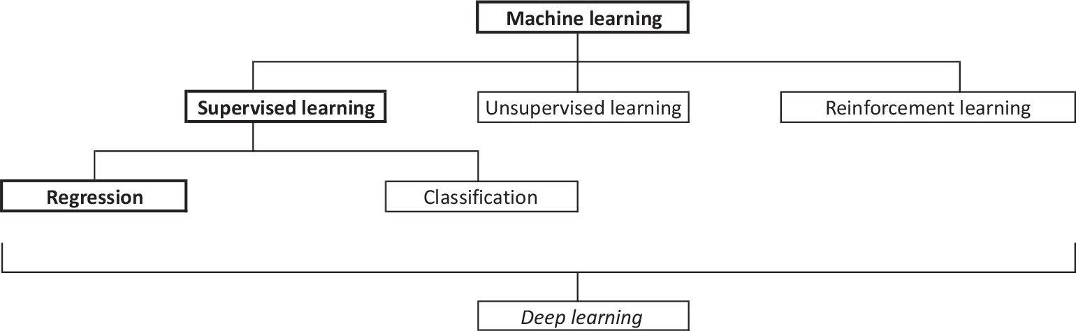
Figure 1. Schematic classification of machine learning methods. The branch leading to regression is in bold since many problems in actuarial science can be expressed as regression problems, as discussed in the next section. Because deep learning models can be used for each of the main branches of machine learning, it spans across the schema.
3.2 Actuarial modelling and machine learning
Actuarial models can often be expressed as regression problems, even if the original problems, at first glance, do not appear to be related to regression. Several obvious and less obvious examples of this are provided in the following points (and in more detail in Table 1):
1. Short-term insurance policies are usually priced with GLM models of frequency (Poisson rate regression) and severity (Gamma regression).
2. The chain-ladder model can be described as a cross-classified log-linear regression according to the GLM formulation of Renshaw & Verrall (Reference Renshaw and Verrall1998).
3. The software implementation of the distribution-free chain-ladder model of Mack (Reference Mack1993) in R (Gesmann et al., Reference Gesmann, Murphy, Zhang, Carrato, Crupi, Wüthrich and Concina2017) uses several linear regression models to estimate the coefficients, but, notably, the entire set of chain-ladder factors can be estimated using a single weighted linear regression.
4. Advanced incurred but not reported (IBNR) models have been fit using generalised linear mixed models (GLMMs) and Bayesian hierarchal models.
5. The comparison of actual mortality to expected experience (AvE) is often performed manually by life actuaries, but this can be expressed as a Poisson regression model where the output is the number of deaths and the input is the expected mortality rate, with an offset taken as the central exposed to risk.
6. The process of determining a life table based on the mortality experience of a company or portfolio is similarly a regression problem, where the outputs are the number of deaths and the inputs are the genders, ages and other characteristics of the portfolio (the estimated coefficients of the model can then be used to derive the mortality rates). An example of a methodology is given in Tomas & Planchet (Reference Tomas and Planchet2014).
7. Currie (Reference Currie2016) showed that many common mortality forecasting models (the Lee-Carter (Lee & Carter, Reference Lee and Carter1992) and CBD (Cairns et al., Reference Cairns, Blake and Dowd2006) models among them) can be formulated as regression problems and estimated using GLM and generalised non-linear models.
8. Richman (Reference Richman2017) showed that the demographic techniques known as the near extinct generations methods (Thatcher et al., Reference Thatcher, Kannisto and Andreev2002), which are used to derive mortality rates at the older ages from death counts, can be expressed as a regression model within the GLM framework.
9. Life insurance valuation models perform cash-flow projections for life policies (or groups of policies, called model points), to allow the present value of future cash flows to be calculated for the purpose of calculating reserves or embedded value. Since running these models can take a long time, so-called “lite” valuation models can be calibrated using regression methods.
10. Another regression problem in life valuations concerns attempts to avoid nested stochastic simulations when calculating risk-based capital, such as in Solvency II or the Swiss Solvency Test. One option is to calibrate, using regression, a reference set of assets, called the replicating portfolio, to the liability cash flows, and perform the required stresses on the replicating portfolio.
Table 1. Feature matrices X and outputs y for several regression problems in actuarial science

Once an actuarial model is expressed as a regression problem, then solutions to the problem are available in the context of machine and deep learning. Thus, taking the above points into consideration, the following (non-exhaustive) heuristic is offered for determining if deep learning solutions (and more broadly, machine learning solutions) are applicable to problems in actuarial science:
If an actuarial problem can be expressed as a regression, then machine and deep learning techniques can be applied.
This heuristic is non-exhaustive, since, as will be shown later, some problems in actuarial science have recently benefitted from the application of unsupervised learning, and, therefore, actuaries faced with a novel problem should also consider unsupervised learning techniques.
The reader is referred to the supplementary appendix for more resources discussing machine learning.
4. An Introduction to Deep Learning
Deep learning is the modern approach to designing and fitting neural networks that relies on innovations in neural network methodology, very large datasets and the dramatically increased computing power available via graphics processing units (GPUs). Although currently experiencing a resurgence in popularity, neural networks are not a new concept, with some of the earliest work on neural networks by Rosenblatt (Reference Rosenblatt1958). Goodfellow et al. (Reference Goodfellow, Bengio and Courville2016) categorise the development of neural networks into three phases:
the early models, inspired by theories of biological learning in the period 1940–1960;
the middle period of 1980–1995, during which the key idea of backpropagation to train neural networks was discovered by Rumelhart et al. (Reference Rumelhart, Hinton and Williams1986); and
the current resurgent interest in deep neural networks that began in 2006, as documented in LeCun et al. (Reference LeCun, Bengio and Hinton2015).
Interest in neural networks declined after the middle period of development for two reasons: firstly, overly ambitious claimsFootnote 5 about neural networks had been made, leading to disappointments from investors in this technology and, secondly, other machine learning techniques began to achieve good results on various tasks (Goodfellow et al., Reference Goodfellow, Bengio and Courville2016). The recent wave of research into neural networks began with a paper by Hinton et al. (Reference Hinton, Osindero and Teh2006) who provided an unsupervised method of training deep networks that outperformed shallow machine learning approaches (in particular, a radial basis function support vector machine; see Chapter 12 in Friedman et al. (Reference Friedman, Hastie and Tibshirani2009) for more on this approach) on a digit classification benchmark (Goodfellow et al., Reference Goodfellow, Bengio and Courville2016). Other successes of the deep learning approach soon followed in speech recognition and pedestrian detection (LeCun et al., Reference LeCun, Bengio and Hinton2015). A breakthrough in computer vision was due to the AlexNet architecture of Krizhevsky et al. (Reference Krizhevsky, Sutskever and Hinton2012) who used a combination of improved computing technology (GPUs), recently developed techniques (rectified linear units (Nair & Hinton, Reference Nair and Hinton2010) and dropout (Hinton et al., Reference Hinton, Srivastava, Krizhevsky, Sutskever and Salakhutdinov2012), which are now used as standard techniques in deep learning) and data augmentation to achieve much improved performance on the ImageNet benchmark using a convolutional neural network (or CNN, the architecture of which is described later). Other successes of deep networks are in the field of natural language processing (NLP), an example of which is Google’s neural translation machine (Wu et al., Reference Wu, Schuster, Chen, Le, Norouzi, Macherey and Macherey2016) and in speech recognition (Hannun et al., Reference Hannun, Case, Casper, Catanzaro, Diamos, Elsen and Coates2014). A more recent example is the winning method in the 2018 M4 time series forecasting competition, which used a combination of a deep neural network (a long short-term network or LSTM Hochreiter & Schmidhuber, Reference Hochreiter and Schmidhuber1997) with an exponentially weighted forecasting model (Makridakis et al., Reference Makridakis, Spiliotis and Assimakopoulos2018). Importantly, although the initial breakthroughs that sparked the recent interest in deep learning were on training neural networks using unsupervised learning, the focus of research and applications more recently is on supervised learning models trained by backpropagation (Goodfellow et al., Reference Goodfellow, Bengio and Courville2016).
This paper asserts that “this time is different” and that the current deep learning research deserves the attention of the actuarial community, not only in order to understand the technologies underlying recent advances in AI but also to expand the capabilities of actuaries and scope of actuarial science. Although actuaries may have heard references to neural networks over the years and may perhaps have even experimented with these models, the assertion of this paper is that the current period of development of neural networks has produced efficient, practical methods of fitting neural networks, which have emerged as highly flexible models capable of incorporating diverse types of data, structured and unstructured, into the actuarial modelling process. Furthermore, deep learning software packages, such as Keras (Chollet, Reference Chollet2015), make the use of these models practical. This assertion will be expanded upon and discussed in this and the following section.
4.1 Connection to AI
Deep learning is a part of the machine learning approach to AI, where systems are trained to recognise patterns within data to acquire knowledge (Goodfellow et al., Reference Goodfellow, Bengio and Courville2016). In this way, machine learning represents a different paradigm from earlier attempts to build AI systems, which relied on hard coding knowledge into knowledge bases, in that the system learns the required knowledge directly from data. Before the advent of deep learning, AI systems had been shown easily to solve problems in formal domains defined by mathematical rules that are difficult for humans, such as the Deep Blue system playing chess. However, highly complex tasks that humans solve intuitively (i.e. without formal rules-based reasoning), such as image recognition, scene understanding and inferring semantic concepts (Bengio, Reference Bengio2009), have been more difficult to solve for AI systems (Goodfellow et al., Reference Goodfellow, Bengio and Courville2016). In the insurance domain, for example, consider the prior knowledge gained by an actuary from discussions with underwriters and claims handlers conducted before a reserving exercise. The experienced actuary is able to use this information to modify her approach to reserving, perhaps by choosing one of several reserving methods, or by modifying the application of the chosen method, perhaps by increasing loss ratios or decreasing claims development assumptions. However, automating the process of decoding the knowledge contained within these discussions, into a suitable format for a reserving model, appears to be a formidable task, mainly because it is often not obvious how to design a suitable representation of this prior knowledge.
In many domains, the traditional approach to designing machine learning systems to tackle these sorts of complex tasks relies on humans to design the feature matrix  $X$, or, as to use the terminology of the deep learning literature (Goodfellow et al., Reference Goodfellow, Bengio and Courville2016), the representation of the data. This feature matrix is then fed to a “shallow” machine learning algorithm, such as a boosted classifier, to learn from the data. For example, a classical approach to the problem of object localisation in computer vision is given in Viola & Jones (Reference Viola and Jones2001), who design a process, called a cascade of classifiers, for extracting rectangular features from images which are then fed into an Adaboost classifier (Freund & Schapire, Reference Freund and Schapire1997) (for a general introduction to boosting, of which the Adaboost classifier is an example, see Chapter 10 in Friedman et al., Reference Friedman, Hastie and Tibshirani2009). An example closer to insurance is within the field of telematics analysis, where Dong et al. (Reference Dong, Li, Yao, Li, Yuan and Wang2016) compare and contrast the traditional feature engineering approach with the automated deep learning approach discussed next. Within actuarial science, another example is the hand-engineered featuresFootnote 6 often used by actuaries for IBNR reserving. During the reserving process, an array of loss development factors (LDFs) is calculated and combinations of these factors, calculated according to various statistical measures and heuristics, are “selected” using the actuary’s expert knowledge. Also, loss ratios are set based on different sources of information available to the actuary, some of which are less dependent on the claims data, such as the insurance company business plan, and some of which are calculated directly from the data, as in the Cape Cod (Bühlmann & Straub, Reference Bühlmann and Straub1983) and generalised Cape Cod methods (Gluck, Reference Gluck1997). These features are then used within a regression model to calculate the IBNR reserves (more discussion of this topic appears in the description of CNNs below).
Designing features is a time-consuming and tedious task and relies on expert knowledge that may not be transferable to a new domain, making it difficult for computers to learn complex tasks without major human intervention, effort and prior knowledge (Bengio & LeCun, Reference Bengio and LeCun2007). In contrast to manual feature design, representation learning, which is thoroughly reviewed in Bengio et al. (Reference Bengio, Courville and Vincent2013), is a machine learning approach that allows algorithms automatically to design a set of features that are optimal for a particular task. Representation learning can be applied in both an unsupervised and supervised context. Unsupervised representation learning algorithms seek automatically to discover the factors of variation underlying the feature matrix  $X$. A commonly used unsupervised representation learning algorithm is PCA which learns a linear decomposition of data into the factors that explain the greatest amount of variance in the feature matrix. An early example of supervised representation learning is the partial least squares (PLS) method, described in Geladi & Kowalski (Reference Geladi and Kowalski1986). After receiving a feature matrix and an output vector, the PLS method calculates a set of new features that maximise the covariance with the response variable using the nonlinear iterative partial least squares (NIPALS) algorithm (Kuhn & Johnson, Reference Kuhn and Johnson2013)Footnote 7, in the hope that these new features will be more predictive of the output than the unsupervised features learned using PCA.
The PCA and PLS methods just described rely on relatively simple linear combinations of the input data. These and similar simpler representation learning methods applied to highly complex tasks, such as speech or image recognition, may often fail to learn an optimal set of features due to the high complexity of the data that the algorithms are analysing, implying that a different set of representation learning techniques are required for these tasks. Deep learning is a representation learning technique that attempts to solve the problem just described by constructing hierarchies of complex features that are composed of simpler representations learned at a shallow level of the model. Returning to the example from computer vision, instead of hand designing features, a more modern approach is to fit a neural network composed of a hierarchy of feature layers to the image dataset. The shallow layers of the network learn to detect simple features of the input data, such as edges or regions of pixel intensity, while the deeper layers of the network learn more complicated combinations of these features, such as a detector for car wheels or eyes. If performed in an unsupervised context, then the network learns a representation explaining the factors of variation of the input data, while if in a supervised context, the learned representation of the images is optimised for the supervised task at hand, for example, a computer vision task such as image classification.
The usefulness of learned representations often extends beyond the original task that the representations were optimised on. For example, a common approach to image classification problems when only small datasets are available is so-called “transfer learning” which feeds the dataset through a neural network that has been pre-trained on a much larger dataset, thus deriving a feature matrix that can then be fed into a second neural network or other classification algorithm, see, for example, Girshick (Reference Girshick2015). A structured data example closer to the problems often solved by actuaries is Guo & Berkhahn (Reference Guo and Berkhahn2016) who tried to predict sales volumes based on tabular data containing a categorical feature with high cardinality (i.e. the feature contained entries for each of many different stores, a problem classically solved by actuaries using credibility theory). After training a representation of the categorical data using neural networks, the learned representation was fed into several shallow classifiers, greatly enhancing their performance. This approach to representation learning represents a step towards general AI, in which machines exhibit the ability to learn intelligent behaviours without much human intervention.
4.2 Definitions and notation
This section now provides some mathematical definition of the concepts just discussed. The familiar starting point, in this paper, for defining and explaining neural networks is a simple linear regression model, expressed in matrix form:
 \begin{equation*}\hat{y} =f\left(X\right)=a+B^{t} X\end{equation*}
where the predictions  $\hat{y}$ are formed via a linear combination of the feature matrix
  $X$, which is derived using a vector of regression coefficients
  $B$ and an intercept term,
  $a$. An example of this simple model is shown in Figure 2 in graphical form, which illustrates a regression model with three features (in this case, the intercept term
  $a$ is illustrated as one of the features, which corresponds to a column set equal to unity in the feature matrix
  $X$). Here, it is helpful to introduce the terminology which is used in the neural network literature: instead of referring to
  $B$ as a vector of regression coefficients, in the neural network literature,
  $B$ is referred to as the weights, and the intercept term
  $a$ is referred to as the bias.

Figure 2. Graph of regression model with three input features and a single output.
In this simple model, the features are used without modification directly to calculate the prediction, although, of course, the feature matrix  $X$ might have benefitted from data transformations or other so-called feature engineering to exploit the data available for the prediction, for example, the addition of interaction effects between some of the variables. An example of an interaction term which might be added to the features in a motor pricing model is the interaction between power-to-weight ratio and gender, which might be predictive of claims. Feature engineering is often performed manually in actuarial modelling and requires an element of judgement, leading to the potential that useful combinations of features within the data are mistakenly ignored.
Neural networks seek to solve the problem of manual feature engineering by allowing the model itself to design features that are useful in the context of the problem at hand. This is performed by constructing a more complex model that includes non-linear transformations of the features. For example, a simple extension of the linear regression model discussed above can be written as:
 \begin{equation*}{Z^1} = {\sigma _0}\left( {{a_0} + B_0^tX} \right)\end{equation*}
 \begin{equation*}\hat{y} =\sigma _{1} \left(a_{0} +B_{1}^{t} Z^{1} \right)\end{equation*}
which states that an intermediate matrix of variables,  ${Z^1}$, is computed from the (input) feature matrix
  $X$, by applying a non-linear activation function,
  ${\sigma _0}$ to a linear combination of the features, which is itself formed by applying a matrix of weights
  ${B_0}$ and a vector of biases
  ${a_0}$ to the input feature matrix
  $X$. A list of popular activation functions appears in Table 2Footnote 8 (the activation functions
  ${\sigma _0}$ are also called ridge functions in mathematics). The intermediate variables
  ${Z^1}$ are referred to as the hidden layer of the network.
Table 2. Popular activation functions

Following this first set of transformations of the variables by the non-linear activation function, the predictions of the model are computed as the output of another non-linear function  ${\sigma_1}$ applied to a linear combination of the intermediate variables
  ${Z^1}$. The only specifications of the intermediate variables are the number of intermediate variables to calculate and the non-linear function – the data are used to learn a new set of features that is optimally predictive for the problem at hand. An example of this model is shown in graphical form in Figure 3, where a model with three input features, four intermediate variables and a bias term, and a single output variable is illustrated (since there are multiple intermediate variables, we refer to
  ${B_0}$ as a matrix and not a vector).

Figure 3. Graph of neural network with a single hidden layer. In this example, there are three input features, a hidden layer consisting of four neurons plus a bias term, and a single output variable.
The last layer of the network is equipped with an activation function designed to reproduce the output of interest; for example, in a regression model, the activation is often the identity function, whereas in a classification model with two classes, the sigmoid activation is used since this provides an output which can be interpreted as a probability (i.e. lies in (0,1)). For multi-class classification, a so-called softmax layer is used, which derives a probability for each class under consideration by converting a vector of real-valued outputs output by a neural network to probabilities.
The model just discussed is a so-called shallow network, since it contains only a single hidden layer (of intermediate variables). Networks that contain two or more hidden layers are referred to as deep networks.
To fit the neural network, a loss or objective function,  $\sum \limits_{i=1}^{n} L\big(y_{i} ,\hat{y} _{i} \big)$, is specified, measuring the quality of (or distance between) the predictions of the model compared to the observations, where the function
  $L()$ can be chosen flexibly based on the problem at hand. For regression, common examples are the MSE or the mean absolute error, while for classification the cross-entropy loss is often used. The model is then fit by backpropagation (Rumelhart et al., Reference Rumelhart, Hinton and Williams1986) and gradient descent, which are algorithms that adjust the parameters of the model by calculating a gradient vector (i.e. the derivative of the loss with respect to the model parameters, calculated using the chain rule from calculus) and adjusting the parameters in the direction of the gradient (LeCun et al., Reference LeCun, Bengio and Hinton2015: Figure 1). In common with other machine learning methods, such as boosting, only a small “step” in the direction of the gradient is taken in parameter space for each round of gradient descent, to help ensure that a robust minimum of the loss function is found. The extent of the “step” is defined by a learning rate chosen by the user. Since the difficulties of performing backpropagation have largely been solved by modern deep learning software, such as the TensorFlow (Abadi et al., Reference Abadi, Barham, Chen, Chen, Davis, Dean, Devin, Ghemawat, Irving, Isard, Kudlur, Levenberg, Monga, Moore, Murray, Steiner, Tucker, Vasudevan, Warden, Wicke, Yu and Zheng2016) or PyTorch (Paszke et al., Reference Paszke, Gross, Chintala, Chanan, Yang, DeVito and Lerer2017) projects, the details are not given but the interested reader can refer to Goodfellow et al. (Reference Goodfellow, Bengio and Courville2016) for a general introduction and to Ruder (Reference Ruder2016) for a review of gradient descent algorithms for neural networks.
The simple model just defined can easily be extended to other more useful models. For example, by replacing the loss function with the Poisson deviance (Wüthrich & Buser, Reference Wüthrich and Buser2018), a Poisson GLM can be fit. More layers can be added to this model to produce a deep network capable of learning complicated and intricate features from the data. Lastly, specialised network layers have been developed to process specific types of data, and these are described later in this section.
Unsupervised learning is also possible, by using a network structure referred to as an auto-encoder (Hinton & Salakhutdinov, Reference Hinton and Salakhutdinov2006). An auto-encoder is a type of non-linear PCA where a (high dimensional) input vector  ${X_i}$ is fed into a neural network, called the encoder, which ends in a layer with only a few neurons. The encoded vector, consisting of these few neurons, is then fed back into a decoding network which ends on a layer with the same dimension as the original vector
  ${X_i}$. The loss function that is optimised is
  $L(X_{i} ,\hat{X}_{i} )$, where
  ${X_i}$ represents the output of the network that is trained to be similar to the original vector,
  ${X_i}$. The structure of this model is shown in Figure 4, where a ten dimensional input is reduced to a single “code” in the middle of the graph.

Figure 4. Graph of an auto-encoder network.
Deep auto-encoders are often trained using a process called greedy unsupervised learning (Goodfellow et al., Reference Goodfellow, Bengio and Courville2016). In this process, a shallow auto-encoder is first trained, and then, the encoded output of the auto-encoder is used as the input into a second shallow auto-encoder network. This process is continued until the required number of layers has been calibrated. A deep auto-encoder is then constructed, with the weights of these layers initialised at the values found for the corresponding shallow auto-encoders. The deep network is then fine-tuned for the application required.
With these examples in hand, some definitions of common terms in deep learning are now given. The idea of learning new features from the data is called representation learning and is perhaps the key strength of neural networks. Neural networks are often viewed as being composed of layers, with the first layer referred to as input layer, the intermediate layers in which new features are computed being referred to as hidden layers, and the last calculation based on the learned features referred to as the output layer. Within each layer, the regression coefficients forming the linear combination of the features are called weights, and the additional intercept terms are called the biases. The learned features (i.e. the nodes) in the hidden layers are referred to as neurons.
An important intuition regarding deep neural network models is that multiple hidden layers (containing variable numbers of neurons) can be stacked to learn hierarchal representations of the data, with each new hidden layer allowing for more complicated features to be learned from the data (Goodfellow et al., Reference Goodfellow, Bengio and Courville2016).
4.3 Advanced neural network architectures
Several specialised layers (convolutional, recurrent and embedding layers) have been introduced allowing for representation learning tailored specifically to unstructured data (images and text, as well as time series), or categorical data with a very high cardinality (i.e. with a large number of categories). Deep networks equipped with these specialised layers have been shown to excel at the tasks of image recognition and NLP, but also, in some instances, in structured data tasks (De Brébisson et al., Reference De Brébisson, Simon, Auvolat, Vincent and Bengio2015; Guo & Berkhahn, Reference Guo and Berkhahn2016). These specialised layers are described in the rest of this section. A principle to consider when reading the following section is that these layers have been designed with certain priors, in the Bayesian sense, or beliefs, in mind. For example, the recurrent layers express the belief that, for the type of data to which they are applied, the information contained in previous data entries has bearing on the current data entry. However, the parameters of these layers are not hand-designed, but learned during the process of fitting the neural network, allowing for optimised representations to be learned from the data.
Note that some advances in neural architectures have not been discussed, mainly because their application is more difficult or less obvious in the domain of actuarial science. For example, generative adversarial nets (Goodfellow et al., Reference Goodfellow, Pouget-Abadie, Mirza, Xu, Warde-Farley, Ozair and Bengio2014), which have been used to generate realistic image, video and text, are not reviewed. Also not discussed are the energy-based models, such as restricted Boltzmann machines which helped to revitalise neural network research since 2006 (Goodfellow et al., Reference Goodfellow, Bengio and Courville2016), but which do not appear to be used much in current practice.
4.3.1. Convolutional neural networks
A convolution is a mathematical operation that blends one function with another (Weisstein, Reference Weisstein2003). In neural networks, convolutions are operations performed on data matrices (most often representing images, but also time series or numerical representations of text) by multiplying elementwise part of the data matrix by another matrix, called the filter (or the convolutional kernel) and then adding each element in the resulting matrix. Convolutional operations are performed to derive features from the data, which are then stored as a so-called feature map. Figure 5 is an illustration of convolution applied to a very simple grey-scale image of a digit. To derive the first digit of the feature map shown in Figure 5, the elementwise product of the first 3 × 3 slice of the data matrix is formed with the filter and the elements are then added.

Figure 5. Illustration of a convolution applied to a simple grey-scale image of a “2”. The 10 × 10 image is represented in the data matrix, which consists of numbers representing the pixel intensity of the image. The filter is a 3 × 3 matrix, which, in this case, has been designed by hand as a horizontal edge detector. The resulting 8 × 8 feature map is shown as another matrix of numbers. The −1 in the top-left corner of the feature map, in grey, is derived by applying the 3 × 3 filter to the 3 × 3 region of the data matrix also coloured in grey. The value is negative one, since the only non-zero entry in this part of the data matrix is 1, which is multiplied by the −1 in the bottom right of the filter. These calculations are shown on the right side of the figure. The same filter is applied in a sliding window over the entire data matrix to derive the feature map.
Many traditional computer vision applications use hand-designed convolutional filters to detect edges. Simple vertical and horizontal edges can be detected with filters comprised of 1, −1 and 0, for example, the filter shown in Figure 5 is a horizontal edge detector. More complicated edge detectors have appeared in the literature, see, for example, Canny (Reference Canny1987). In deep learning, however, the weights of the convolutional filters are free parameters, with values learned by the network and thus avoiding the tedious process of manually designing feature detectors. Goodfellow et al. (Reference Goodfellow, Bengio and Courville2016) provide the following intuition for understanding CNNs: suppose that one placed an infinitely strong prior (in the Bayesian sense) on the weights of a neuron, that dictated, firstly, that the weights were zero except in a small area and secondly, that the weights of the neuron were the same as the weights of its neighbour, but that its inputs were shifted in space. This would imply that the learned function should only learn local features from the data matrix and that the features detected in an object should be detected regardless of their position within the image. This prior is ideal for detecting features in an image, where specific components will vary in space and the components do not occupy the entire image.
The modern application of CNNs to image data generally involves the repeated application of convolutional layers followed by pooling layers, which replace the feature map produced by the convolutional layer with a series of summary statistics (Goodfellow et al., Reference Goodfellow, Bengio and Courville2016). This induces translation invariance into the learned features, since a small modification of the image will generally not affect the output of the pooling layer. The multiple layers of convolution and pooling are generally followed by several fully connected layers, which are responsible for using the features calculated earlier in the network to classify images or perform other tasks. Figure 6 shows a simple CNN applied to a tensor (matrix with multiple dimensions) of 3 × 128 × 128, in which the first dimension is typical of RGB images which have three channels.

Figure 6. A simple convolutional network applied to a 3 × 128 × 128 tensor, the first dimension of which is characteristic of images where the pixels are defined on the RGB scale.
As documented in LeCun et al. (Reference LeCun, Bengio and Hinton2015), CNNs are not new concepts, with an early example being LeCun et al. (Reference LeCun, Bottou, Bengio and Haffner1998). CNNs fell out of favour until the success achieved by the relatively simple modern architecture in Krizhevsky et al. (Reference Krizhevsky, Sutskever and Hinton2012) on the ImageNet challenge. Better performing architectures with exotic designs and idiosyncratic names have been developed more recently; an early example of these exotic architectures is the “Inception” model of Szegedy et al. (Reference Szegedy, Liu, Jia, Sermanet, Reed, Anguelov and Rabinovich2015).
Although this discussion and the illustration in Figure 5 relates to the analysis of images, which is not a common task for actuaries, it is notable that convolutional networks have been applied successfully in several domains that actuaries may be interested in. For example, Gao & Wüthrich (Reference Gao and Wüthrich2019) use a CNN to identify drivers from telematics information, and more generally, convolutional networks have been used for time series forecasting, see Borovykh et al. (Reference Borovykh, Bohte and Oosterlee2017). We discuss a potential application of these networks for IBNR reserving in the next section.
4.3.2. Parallel to IBNR reserving
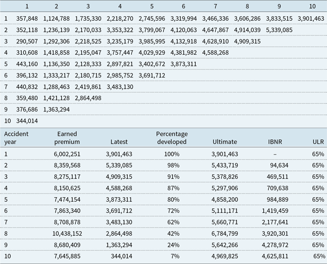
An interesting parallel between CNNs and the derivation of features for input into IBNR reserving methods (algorithms) can be drawn. The famous triangle of claims appearing in Mack (Reference Mack1993) and shown, together with the chain-ladder calculations, performed using the ChainLadder package (Gesmann et al., Reference Gesmann, Murphy, Zhang, Carrato, Crupi, Wüthrich and Concina2017) in R, as well as earned premium estimated to provide a long-run ultimate loss ratio (ULR) in each year of 65%, appears in Table 3.
Table 3. Claims triangle from Reference MackMack (1993) and the chain-ladder calculations
Consider applying a simple 1 × 2 convolutional filter, consisting of the matrix  $[{-}1\ 1]$, to the triangle, after undergoing one of two transformations. In the first, the (natural) logarithm of the entries in the triangle not equal to zero is taken and, in the second, the entries are divided by the earned premium, relating to each accident year, to derive the cumulative loss ratios, and then the convolution is applied. The resulting feature matrices are shown in Table 4. The first matrix consists of the logarithm of the individual (i.e. relating to a single accident year) LDFs from the chain-ladder method, and the second shows the incremental loss ratios used in the additive loss ratio method described in Mack (Reference Mack2002). That the features underlying some of the most popular algorithms for reserving are relatively simple is not surprising, since these methods are engineered to produce forecasts using weighted averages of the features. However, the possibility exists that a deep neural network might find more predictive features if trained on enough data.
Table 4. Feature matrices derived by applying a 1 × 2 convolution filter to the triangle shown in Table 3, adjusted as described in the text. The first matrix shows the (natural) log LDFs, and the second shows the incremental loss ratios

4.3.3. Recurrent neural networks
The architectures discussed to this point have been so-called feed-forward networks, in which the various hidden layers of the network are recalculated for each data point and the hidden “state” of the network is not shared for different data points (i.e. there are no connections between hidden layers computed on different data points). Many data types, though, form sequences and a full understanding of the individual entries of the sequences is only possible within the context provided by the other entries. Examples of these types of data are time series, natural language and video data. The problem of maintaining the information gained about the context from previous data points is addressed by recurrent neural networks (RNNs), which can be imagined as feed-forward networks that share the state of the hidden variables from one data point to another. Whereas feed-forward networks map each input to a single output, RNNs map the entire history of inputs to a single output (Graves, Reference Graves2012) and thus can build a so-called “memory” of the data points that have been seen.
A common simplifying assumption of actuarial and statistical models is the Markov assumption, which can be stated simply as saying that once the most recent time step of the data or parameters is known, the previous data points and parameters have no further bearing on the model. RNNs allow this assumption to be relaxed (Goldberg, Reference Goldberg2017) by storing the parts of the history, shown to be relevant, within the network’s internal memory.
Since RNNs are designed for the processing of observations that occur over time, we use a somewhat different notation in this section than previously. Here, we consider that the columns of the feature matrix  $X$ consist of observations of the same variable at different times,
  $t\; \in \;\left[ {1,...,T} \right]$. Thus, we represent the
  $i$th example of the time series with observation at time
  $t$ as
  ${X_{i,t}}$ and the output at each time step that the network is trained to reproduce is
  ${y_{i,t}}$. Similarly, since RNNs process observations over time, a somewhat different way of representing these graphically networks is required. The two common forms of representing an RNN are shown in Figure 7, with the so-called “folded” representation on the left of the figure, and the “unfolded” (over time) representation on the right. The diagram shows that RNNs contain a feedback loop that allows the value of the hidden layer of the network at one point in time to be fed to the network at the next point in time. The figure shows a simple RNN that was proposed by Elman (Reference Elman1990). It should be noted that this figure is a simplification and multi-dimensional inputs into and out of the network are possible, as well as multiple RNN layers stacked on top of each other. Also, nothing precludes using the output of another neural network as the input into an RNN or vice versa, for example, LeCun et al. (Reference LeCun, Bengio and Hinton2015: Figure 3) provide an example of an image captioning network which takes, as an input to the RNN, the output of a CNN and produces, as an output of the RNN, image captions.

Figure 7. Common graphical representations of a recurrent neural network, which is being applied to process an input vector  $x_i$, that has multiple observations over time. This diagram is different from the networks illustrated previously, in that values input to the network appear at the bottom of the diagram. The narrow vertical arrows show the input vector
  $x_i$ being processed by the network, which then returns an output,
  $O$. The wide arrow shows that the hidden layers of the network are connected to each other. The graph on the left shows a folded form of the RNN, and the graph on the right shows the same RNN unfolded over time, with the observation at time
  $t$ is denoted as
  ${x_t}$. At each step, the parameter values are shared. Note that the inputs to the RNN can be multi-dimensional, the actual RNN can have many layers, and the outputs can be fed into other types of network architectures.
When one views RNNs in the “unfolded” representation, it can be seen that RNNs are a form of deep neural network. Whereas the deep networks discussed to this point use multiple hidden layers to process a single observation, here multiple hidden layers are used to process a sequence of observations, in other words, these networks are deep when the time dimension of the network is considered (which is different from the other networks discussed above) (Goldberg, Reference Goldberg2017). For more discussion of the concept of depth in RNNs, see Pascanu et al. (Reference Pascanu, Gulcehre, Cho and Bengio2013). To train RNNs, a modified version of the backpropagation algorithm is used. Recalling the discussion in Section 4.2, gradient descent is usually applied to train neural networks, with the gradients calculated using the backpropagation algorithm. In the case of RNNs, the gradients are estimated over the time steps of the network using the so-called backpropagation over time (Werbos, Reference Werbos1988).
Although RNNs are conceptually attractive, they proved difficult to train in practice due to the problem of either vanishing, or exploding, gradients (i.e. when applying backpropagation to derive the adjustments to the parameters of the network, the numerical values that are calculated do not provide a suitable basis for training the model) (LeCun et al., Reference LeCun, Bengio and Hinton2015). Intuitively, backpropagation is similar to the chain rule in calculus, and by the time the chain rule calculations reach the earliest (in time) nodes of the RNN, the weight matrix that defines the feedback loop shown in Figure 7 has been multiplied together so many times that the gradients are no longer accurate.
Other, more complicated, architectures that do not suffer from the vanishing or exploding gradient problem are the LSTM (Hochreiter & Schmidhuber, Reference Hochreiter and Schmidhuber1997) and gated recurrent unit (GRU) (Chung et al., Reference Chung, Gulcehre, Cho and Bengio2015) designs. An intuitive explanation of these so-called “gated” designs is that, instead of allowing the hidden state automatically to be updated at each time step, updates of the hidden state should occur only when required (as learned by the gating mechanism of the networks from the data), creating a more stable feedback loop in the hidden state cells than a simple RNN. The influence of earlier inputs to the network is therefore maintained over time, thus mitigating the training issues encountered with simple RNNs (Goodfellow et al., Reference Goodfellow, Bengio and Courville2016; Graves, Reference Graves2012). For more mathematical details of LSTMs and GRUs and explanation of how these architectures solve the vanishing/exploding gradient problem, the reader is referred to Goodfellow et al. (Reference Goodfellow, Bengio and Courville2016: Section 10.10). These details may appear complicated, and perhaps even somewhat fanciful on a first reading, however, key is that LSTM and GRU cells, which are useful for capturing long-range dependencies in data, can easily be incorporated into a network design using modern software, such as Keras.
RNNs have achieved impressive success in many specialised tasks in NLP (Goldberg, Reference Goldberg2017), machine translation (Sutskever et al., Reference Sutskever, Vinyals and Le2014; Wu et al., Reference Wu, Schuster, Chen, Le, Norouzi, Macherey and Macherey2016), speech recognition (Graves et al., Reference Graves, Mohamed and Hinton2013) and, perhaps most interestingly for actuaries, time series forecasting (Makridakis et al., Reference Makridakis, Spiliotis and Assimakopoulos2018), in combination with exponential smoothing.
4.3.4. Embeddings
Machine learning algorithms generally rely on the one-hot encoding procedure, which is often called dummy coding by statisticians, when dealing with categorical data. In this encoding scheme, vectors of categorical features are expanded into a set of indicator variables, all of which are set to zero, except for the one indicator variable relating to the category appearing in each row of the feature matrix. When applied to many categories, one-hot encoding produces a high-dimensional feature matrix that is sparse (i.e. many of the entries are zero), leading to potential difficulties in fitting a model as there might not be enough data to derive credible estimates for each category. Modelling categorical data with high cardinality (i.e. when the number of possible categories is very large) is a task that has been addressed in detail in actuarial science within the framework of credibility theory; see, for example, Bühlmann & Gisler (Reference Bühlmann and Gisler2006) for a detailed discussion of the Bühlmann–Straub credibility model. Credibility models do not rely exclusively on the observations available for each category, but rather produce pooled estimates that lie between the overall mean and the observation for each category, thus sharing information across categories. In statistics, GLMMs are an extension of standard GLMs to include variables that are not modelled solely on the basis of the observed data, but rather using distributional assumptions that lead to similar formulae as credibility theory (for the interested reader, Gelman & Hill (Reference Gelman and Hill2007) is an easy introduction to GLMMs and Chapter 12 of this book contains discussions that are highly reminiscent of credibility theory).
The problem of modelling high-dimensional and sparse data is particularly acute in NLP (Bengio et al., Reference Bengio, Ducharme, Vincent and Jauvin2003), where words in a corpus of text are often represented by sparse integer-valued features (i.e. one-hot encoding) or more complicated features called n-grams which are essentially small phrases of  $n$ words that are grouped together (e.g. in the sentence “The quick brown fox jumps over the lazy dog,” the first 3-gram is the phrase “The quick brown”). N-grams use the context of words appearing together in sentences to help reduce the dimensionality of the language modelling problem but suffer from two main problems. Firstly, the contexts used are often short (i.e. 1-gram, i.e. one-hot encoding, or 2-gram schemes are often used), and the similarity between words is not accounted for (i.e. the feature vectors used in the models are orthogonal to each other by design). The insight of Bengio et al. (Reference Bengio, Ducharme, Vincent and Jauvin2003) to solve these problems is that language data can successfully be encoded into low-dimensional, dense numerical vectors which can be trained using neural networks. These vectors are trained to be close to each other (in the vector space) if the words are similar and distant if they are not, thus, the model of the language data learns to associate correlated words and “gains statistical strength by sharing parameters” (Goldberg, Reference Goldberg2016: 351) which is accomplished by allowing the model to treat words with similar features in a common way (Goodfellow et al., Reference Goodfellow, Bengio and Courville2016). These concepts, on which many NLP applications are based, are similar to the idea of actuarial credibility methods that share information across similar categories, as mentioned above. In NLP, embeddings are often pre-trained on a large corpus of text and then applied to specific tasks, and many researchers have made pre-trained embeddings freely available in the Internet.
Embeddings have been used in wider contexts than NLP, two examples of which are De Brébisson et al. (Reference De Brébisson, Simon, Auvolat, Vincent and Bengio2015) and Guo & Berkhahn (Reference Guo and Berkhahn2016). In the context of predicting taxi destinations based on a number of categorical variables and global positioning system data, De Brébisson et al. (Reference De Brébisson, Simon, Auvolat, Vincent and Bengio2015) build a network with separate embeddings for each categorical variable, which was the winning solution in the Kaggle Taxi Service Prediction problem. Guo & Berkhahn (Reference Guo and Berkhahn2016) discuss embeddings in the context of the Kaggle Rossmann Sale Prediction competition. Their model consists of several embeddings of categorical variables concatenated together into a single layer, on top of which were placed two fully connected layers. The model was trained to predict daily sales for each Rossmann store, and the model was tested on two versions of the dataset – one shuffled, and one unshuffled, so that more recent entries appeared towards the end of the dataset. On the shuffled dataset, using embedding layers did not boost the performance of the neural network significantly compared to using one-hot encoding, whereas on the unshuffled dataset, the embeddings provided a relatively small boost in performance. The trained embeddings were then used in other shallow classifiers, and, compared to the one-hot encoded features, provided a major boost in performance, that is, the out-performance of the deep networks was due to the learned feature representation for the categorical data.
Goldberg (Reference Goldberg2016: Section 4.6) provides some intuition why an embedding layer might not result in better performance in a neural network. When categorical features have been one-hot encoded, the first layer of the neural network will learn a representation of all of the features together that is comparable to an embedding layer, thus, the differences between the approaches are potentially more subtle than would initially appear. The key difference seems to be that embedding layers allow a dense representation to be learned separately for each feature before being combined in the neural network, and, along these lines, Guo & Berkhahn (Reference Guo and Berkhahn2016) note that embedding layers allow the network to learn the intrinsic properties of each feature as well as learning about the output distribution.
Embeddings are often visualised using dimensionality reduction algorithms such as PCA or t-SNE (Maaten & Hinton, Reference Maaten and Hinton2008) and often reveal surprisingly intuitive properties of the learned embeddings. Interesting examples of such a visualisation is Figure 2 in Mikolov et al. (Reference Mikolov, Sutskever, Chen, Corrado and Dean2013), which shows that the embedding layers have learned a semantic relationship relating capital cities to the countries in which they are found and Figure 3 in Guo & Berkhahn (Reference Guo and Berkhahn2016) which shows that the embedding of store locations has learned a representation suggestive of the map of Germany (in which the Rossmann stores are located).
5. Conclusions
This section has provided a summarised review of representation learning, deep neural networks and their connection to AI, and specialised architectures for dealing with image, text and categorical data. At this point, we refer the reader back to Table 1, to consider what an enhanced feature matrix for common actuarial problems, expressed as regression models, could potentially comprise. Some examples of enhanced feature matrix are as follows.
Using CNNs, image data can be easily incorporated into the actuarial modelling process if this was considered to be predictive.
Textual data, for example, description of risks or claims handlers’ notes, could be incorporated into the pricing and reserving process using RNNs and word embeddings.
Categorical data in actuarial models (e.g. brands of cars and product types) can be modelled with embeddings, potentially enhancing predictive power.
Having introduced the key concepts of machine and deep learning in this paper, we refer the reader to Part 2 in the companion paper which explores recent attempts to incorporate neural networks into actuarial models.
Supplementary materials
To view supplementary material for this article, please visit https://doi.org/10.1017/S1748499520000238


