1. INTRODUCTION
Coordinate measuring machines (CMMs) are measuring devices that make possible the evaluation of dimensional values of geometrically sophisticated workpieces. During the coordinate measuring process the object to be measured is normally probed point by point using a stylus with a spherical (most commonly) ruby ball tip. At each probing contact, the XYZ coordinates of the ball tip are measured and stored in a computer's memory. The sensor, which provides the connection between the object surface and the 3-D length measuring system of the CMM, is called a “probe.” There are groups of contacting (touch) and noncontacting (optoelectronic) probing systems (Weckenmann et al., Reference Weckenmann, Estler, Peggs and McMurtry2004). A number of different optoelectronic probes are used, although triangulation probes are most popular. Touch probes are categorized into trigger and measuring (scanning) probes. Contacting probes are categorized into touch trigger and measuring systems. Touch trigger probes are most widely used, and are the devices used in this research paper.
The probe is one of the most important factors influencing CMM accuracy (Nawara & Sladek, Reference Nawara and Sladek1985; Krejci, Reference Krejci1990; Butler, Reference Butler1991; Reid, Reference Reid1992; Mayer et al., Reference Mayer, Ghazzar and Rossy1996; Chan et al., Reference Chan, Davis, King and Stout1997; Cauchick-Miguel & King, Reference Cauchick-Miguel and King1998; Johnson et al., Reference Johnson, Yang and Butler1998; Miguel et al., Reference Miguel, King and Abackerli1998). It is very important for the user to have the possibility of verifying probe accuracy after it has been used over a period of time. Furthermore, comparison of the metrological feasibilities of different kinds of probes is valuable. Until now, methods used to calibrate the CMM have relied on manually checking the probes with standard material (calibration artefacts), such as a ring or a ball (ANSI/ASME, 1989; VDI/VDE, 1989; Mayer et al., Reference Mayer, Ghazzar and Rossy1996; Miguel et al., Reference Miguel, King and Abackerli1998; ISO, 2001). However, these techniques are not precise enough because the accuracy of the machine is in most cases comparable with the accuracy of the probe.
One possible solution is to apply a method that allows separation of machine and probe errors. Nafi et al. (Reference Nafi, Mayer and Wozniak2011) have developed CMM-based implementation of the multistep method for such separation. According to the authors, at least for the two-dimensional error pattern, some on-machine testing and error decoupling is possible.
A more precise description of probe accuracy can be achieved by outright testing on special setups, separate from the CMM (Burdekin et al., Reference Burdekin, Di Giacomo and Xijing1985; Nawara & Sladek, Reference Nawara and Sladek1985; Harary et al., Reference Harary, Creimeas, Chollet and Clement1989; Dobosz & Ratajczyk, Reference Dobosz and Ratajczyk1994; Mayer et al., Reference Mayer, Ghazzar and Rossy1996; Dobosz & Woźniak, Reference Dobosz and Woźniak2003; Woźniak & Dobosz, Reference Woźniak and Dobosz2003). Several attempts were made to give a simple and adequate description of the CMM probe (Butler, Reference Butler1991; Estler et al., Reference Estler, Phillips, Borchardt, Hopp, Witzgall, Levenson, Eberhardt, McClain, Shen and Zhang1996; Mayer et al., Reference Mayer, Ghazzar and Rossy1996; Woźniak & Dobosz, Reference Woźniak and Dobosz2005), and to develop a method to test them outside the machine, with mixed results.
Research done by Butler (Reference Butler1991) has shown that the measuring probe is a source of 60% of errors of measurements performed on a coordinate machine, and that it is possible to improve precision by developing models of pretravel variation that consider the character of these errors. Yang et al. (Reference Yang, Butler and Baird1996) have proposed a model of probe pretravel switching which includes a series of parameters: location of the probe in space, measuring force (usually set by adjusting the probe tip spring preload), configuration of the measurement stylus (including weight, length, and rigidity of its tip), direction of switching, together with ambient conditions such as temperature gradients, humidity, and others. Shen and Moon (Reference Shen and Moon1997) have performed similar research studies, by using neural networks having reverse propagation apt to correct the triggering probes errors. Following the authors, thanks to neural network use, a considerable reduction of systematic probe errors has been achieved. Tyler Estler and Shen have developed a mathematical model of kinematic groups of switching probes (Estler et al., Reference Estler, Phillips, Borchardt, Hopp, Witzgall, Levenson, Eberhardt, McClain, Shen and Zhang1996, Reference Estler, Phillips, Borchardt, Hopp, Levenson, Eberhardt, McClain, Shen and Zhang1997). The theoretical description of a probe transducer includes elastic deflections of the probe tip and a friction phenomenon that appears between the spherical tip of the measuring probe and the measured element when locating the measured points on the coordinate machine. The theoretical analysis has been limited to a simplified model of a kinematic triggering probe transducer equipped with a straight measuring tip. A possible extension of this method is the use of the kinematic model proposed by Wozniak and Dobosz (Reference Woźniak and Dobosz2005). Mayer et al. (Reference Mayer, Ghazzar and Rossy1996) have shown another approach to numerical compensation of systematic probe errors. Their target was to generate a simple model, supported by a lesser number of possible parameters. It was assumed that the diagram of repeatability in the probe operating plane is the main characteristic that describes the precision of probe performance. The considerations assumed that during the measurement carried out on a coordinate machine, the probe tip displaces mainly orthogonally to its axis at the moment of contact with the measured object. Balazinski and Mayer have proposed a manually constructed fuzzy decision support system that allows corrections of pretravel variations (Balazinski et al., Reference Balazinski, Czogala, Mayer and Shen1997). They limited their analysis to the electromechanical probes. We present an alternative approach to the problem, including the consideration of two stage probes.
In this paper the authors investigate the use of genetically generated 3-D fuzzy models of the accuracy of touch trigger probes. In addition, current information pertaining to known parameters generally specifies the probe accuracy in the plane perpendicular to the probe axis. This information is extended to include 3-D space in this paper.
More precisely, the genetically generated fuzzy knowledge bases (FKBs) are used for reconstruction of the direction-dependent probe error, that is, the pretravel w. The pretravel is measured according to its definition as the displacement of the stylus tip between the point of touch with a workpiece and the triggering moment. In FKB, w represents the output variable while setting angles β and γ are used as input variables. Angles β and γ describe the spatial direction of probe triggering (normal to the measured surface). Further details will be given later in this paper.
The FKBs developed in this research can be used for automatic or manual calibrations of the CMM. The transparency of the databases and rule bases of FKB, as opposed to black-boxed approaches like neural networks, adds to the knowledge about the link between the measured parameters (inputs of the fuzzy models) and the calibration error (output of the fuzzy model) through the fuzzy rules (FRs) that represent the relationships between the input parameters and the output parameter.
This paper starts with an introduction, followed by a research aim. Section 3 is a brief description of touch trigger systems followed by Section 4, which describes the measurement method. Section 5 describes the experimental setup, whereas Section 6 explains the learning data collection using the experimental setup. Section 7 describes the genetic fuzzy learning environment, followed by Section 8, which presents the generation of the fuzzy models; Section 9 describes their validation. The paper ends with a conclusion followed by acknowledgments and a set of references.
2. RESEARCH AIM
Over the past 20 years remarkable progress in coordinate measurement technology can be noticed in electronic elements (controllers) and in machine software. The use of modern controllers and measurement algorithms allows a remarkable improvement in the measurement precision of coordinate machines, and is performed by numerical compensation of systematic errors of measuring transducers. Currently, in all coordinate machines a compensation of average error is used; it is calculated during the calibration process using a master sphere before performing the proper measurements. The effective radius of the sphere probe tip is calculated, considering five (or more) measurement points of the master sphere; thus extracting an average error value. However, this way of determining the average error value, based upon a few random measuring points is not precise enough because this procedure does not include information about the character of systematic errors of the probes.
The main aim of this research paper is to develop a FKB to model and subsequently correct probe error variation. A secondary research aim is to define the suitable minimal number of setups for CMM machines for error calibration. Furthermore, the FRs bases of the FKB are analyzed to better understand the relationships between geometric/physical setups of the CMM and measuring errors represented by the pretravel value.
3. TOUCH-TRIGGER SYSTEMS
All touch-trigger probes for CMMs contain a three-base spring-tighten setting mechanism (a six-point kinematic mechanism) by which the stylus is electrically fixed in 5 or 6 spatial degrees of freedom. In the basic version this mechanism is designed as a group of electrical contacts (see Fig. 1a). When the stylus touches a workpiece the electrical contact is opened and a trigger pulse is generated and sent to the computer resulting in a coordinate reading. Although there are many different designs of this kind of probe, the generation of the trigger pulse is always strictly connected with a triploid structure of the settings. Setting points are always displaced by 120o, and for this reason the probing force is not uniform. In addition, different values of stylus displacement from the neutral position to the triggering position, depending on probing direction, are observed. As a result, when measuring a circle, a triangular form error will occur.

Fig. 1. The scheme of the touch trigger probes: (a) one-stage type with electromechanical transducer and (b) two-stage type with three piezo elements.
Three base setting probes with electrical contact transducers are the most popular because of their simplicity and low cost. Because they contain only one kind of transducer, they are called one-stage probes or electromechanical probes. To avoid the above-mentioned drawbacks of one-stage probes, piezoelectric sensors are employed in addition to mechanical/electrical contacts (see Fig. 1b). This provides constant sensitivity in all probing directions in the plane perpendicular to the stylus, which effectively reduces probing errors. In the two-stage probe, a very sensitive piezo-element acts as an actual position sensor (first stage), and the electromechanical contact (second stage) only serves to confirm the workpiece probing action.
As a 3-D model of the touch trigger probe 3-D pretravel, Estler et al. (Reference Estler, Phillips, Borchardt, Hopp, Witzgall, Levenson, Eberhardt, McClain, Shen and Zhang1996) presented a first attempt to create a simple mechanical common model of touch-trigger probe. They limited their analysis to electromechanical probes. An alternative approach to the calibration problem is presented in this paper, using FKBs and applying them to one- and two-stage probes.
In the case of one-stage probes the error is a function of switching direction, defined in the space by the two angles. In the case of probes with a piezoelectric transducer, the error in the orthogonal plane to the probe axis does not depend on measurement direction.
4. MEASUREMENT METHOD
A method developed by Woźniak and Dobosz (Reference Woźniak and Dobosz2003) applying a low-force high-resolution displacement transducer is proposed to measure triggering probe pretravel w in XYZ space. The idea relies on detection of contact of a stylus tip with an element that activates its operation (i.e., a measured workpiece). As defined above, the pretravel is the displacement between the point of touch of the workpiece and the triggering moment. The spatial distribution of points obtained by probe triggering from different directions in XYZ space delivers information on probe accuracy. The moment of contact of the probe tip with the element that initiates its movement is detected by means of a low-force displacement transducer. The transducer tip contacts the probe tip before the measurement of pretravel length is realized. The thrust induced by the transducer must be at least 10 times lower than the probe thrust in order to prevent activating the probe. The measurement starts from determination of the position of the transducer measuring arm in the neutral position, which corresponds to the moment when the displacement transducer tip touches the probe tip. When the probe is mechanically triggered by external force the transducer reading is recorded. The difference in readings is the measure of the pretravel (w).
5. EXPERIMENTAL SETUP
The experimental setup employing the low-force displacement transducer with a hinged arm is shown in Figure 2. The high-resolution interference displacement transducer with a low measuring force is the key part of the system. The applied gauge was equipped with a rotary measuring arm as described in Dobosz (Reference Dobosz1994a, Reference Dobosz1994b). The measuring range of the displacement transducer was equal to 4 mm, with a resolution of about 0.015 µm. The measuring force was about 5 mN and varied less than a few percent within the whole measuring range. In order to reach such a low measuring force the following precautions were taken: a precise ball bearing was used on the transducer measuring arm, moving elements made of magnesium alloy were used to ensure a low moment of inertia and a precise balance of the system was completed.

Fig. 2. (a) A schematic and (b) photo of the experimental setup. [A color version of this figure can be viewed online at journals.cambridge.org/aie]
Because the applied measuring force of the displacement transducer is a few dozen times lower than the thrust required to trigger the probe (at least 100 mN lower) it can be assumed that the mutual interaction of the tips of the measuring head and the tested probe is negligible. The external driving unit used to change the position of the tested probe comprises a carriage and its drive. Flat faces of the carriage do not affect the tip of the tested probe directly but by means of the rotary arm of the interference measuring head. The arm ends with a flat surface from one side and ball shaped from the other. Thus, it can interact both with the ball tip of the tested probe and the flat face of the driving unit. The arm transfers the movement to the tip of the tested probe. The carriage performs a to and from motion resulting in triggering the tested probe. Information related to the path that the tip has traveled from the neutral position to the triggering point is registered at the moment of triggering and the results are recorded in a computer.
The measuring system allows changing the approach angle of the probe in the 3-D space. It is realized by rotation of the probe along its axis (angle β in Fig. 2) and by tilting the probe holder in the plane YZ of the measuring system (angle γ in Fig. 2) using the index head.
The measuring system is controlled by computer software that also calculates parameters and characteristics of the tested probes as well as stores data on a hard disc and/or presents them in a form of printed protocols.
The settings of the described measuring system are as follows:
• the angle β of rotation of the probe around its axis during measurement in the measuring setup extending from 0° to 351°,
• the minimum angle of rotation of the probe around its axis during measurement equal to 1.8°,
• the angle γ of rotation of the probe during measurement in the YZ plane of the measuring system extending from 0° to 90°,
• the minimum angle of revolution of a probe in the YZ plane during measurement equal to 1°, and
• the carriage velocity in a probe triggering mode controlled within the range from about 3.1 to about 9.5 mm/s.
6. COLLECTING THE EXPERIMENTAL LEARNING DATA
The 3-D characteristics of pretravels are values of the pretravel as a function of the approaching direction of a stylus tip to a contact with a surface of a measured workpiece.
In this paper the full 3-D pretravel characteristics of various one- and two-stage probes were measured. The probes were tested in their standard configuration and commonly used styluses were utilized. The stems were 40 mm long and 2 mm in diameter, and were made of tungsten carbide with a 4-mm sapphire ball at the end. For the probes with adjustable spring pressure the transducer thrust was set in the middle of the range. The measuring velocity of the majority of CMMs (which is also the probe triggering velocity) can be adjusted from 1 to a few 10s of millimeters per second. In our experiments we applied a value of 8 mm/s, which is the most typical speed used for probe tests by Renishaw.
Test runs comprising five measurements of pretravel were done for both probes considered in this paper. The tip approaching direction in space was changed by 9o for every consecutive measurement. In total, 2000 measurement points were obtained for each probe. Figure 3 and Figure 4 show spatial distributions of the average error plotted in Cartesian coordinates for the switching probe TP6 and the double-stage probe TP200, respectively. Angle β represents the angle of triggering force direction in the XY plane perpendicular to the probe axis, whereas angle γ is the angle between triggering force direction and the XY plane.

Fig. 3. An example of spatial distributions of the average pretravel of the electroswitching probe TP6 plotted in Cartesian coordinates. [A color version of this figure can be viewed online at journals.cambridge.org/aie]

Fig. 4. An example of spatial distribution of the average pretravel of two-stage probe TP200 plotted in Cartesian coordinates. [A color version of this figure can be viewed online at journals.cambridge.org/aie]
7. AUTOMATIC GENERATION OF FKB
Genetic algorithms (GAs) are powerful stochastic optimization techniques based on the analogy of the mechanics of biological genetics and imitate the Darwinian survival of the fittest approach (Goldberg, Reference Goldberg1989). Each individual of a population is a potential fuzzy decision support system FKB, where four basic operations of the developed GA learning software are performed: reproduction, mutation, evaluation, and natural selection. The GA developed by the authors is a combination of a real coded genetic algorithm and a binary coded genetic algorithm called a real binary/like coded genetic algorithm (RBCGA; Achiche et al., Reference Achiche, Baron and Balazinski2003, Reference Achiche, Baron and Balazinski2004b). The reproduction mechanism is a multicrossover proposed by the authors (Achiche et al., Reference Achiche, Baron and Balazinski2004b; Achiche, Balazinski, & Baron, Reference Achiche, Balazinski and Baron2004) and the mutation is uniform as proposed by Cordon et al. (Reference Cordon, Herrera and Villar2000).
7.1. Performance criterion of RBCGA
The performance criterion allows computation of the rating of each FKB used by the RBCGA to perform natural selection. In this paper, the performance criterion is the accuracy level of FKB (approximation error) in reproducing the outputs of the learning data. The approximation error is a combination of the ΔRMS, measured using the root mean square (RMS) error method and the average absolute error ΔABS. The next two equations detail these errors.
 $$\Delta _{{\rm RMS}} = \sqrt {\sum\limits_{i = 1}^N {\displaystyle{{\left({{\rm RBCGA}_{{\rm output}} - {\rm data}_{{\rm output}} } \right)^2 } \over N}\ } }\comma\eqno\lpar 1\rpar$$
where N represents the size of the learning data. The absolute error is measured as follows:
 $$\Delta _{{\rm ABS}} = {\sum\limits_{i = 1}^N {\displaystyle{{{\rm ABS}\left({{\rm RBCGA}_{{\rm output}} - {\rm data}_{{\rm output}} } \right)} \over N}\cdot} } \eqno\lpar 2\rpar$$
The fitness value ϕ is evaluated as a percentage of the output length of the conclusion L, that is,
 $${\rm \phi} = \left({1 - \displaystyle{{\Delta _{{\rm RMS}} + \Delta _{{\rm ABS}} } \over {2L}}} \right)\times 100.\eqno\lpar 3\rpar$$
7.2. Evolutionary strategy of RBCGA
The multiple crossovers per couple (MCPC) strategy is used on the reproduction mechanisms as the evolutionary strategy.
The MCPC consists of the exploration/exploitation balance strategy proposed by the authors (Achiche et al., Reference Achiche, Baron and Balazinski2004a; Achiche, Balazinski, & Baron, Reference Achiche, Balazinski and Baron2004). This strategy is applied to ensure good balance between exploitation and exploration throughout the evolution. Different values were given to the Exploitation/Exploration parameter α that influences the exploration, exploitation or relaxed exploitation levels of the crossover mechanism. These values are set as follows:
• Exploration: α = 1.00 for exploration only
• Relaxed exploitation: α = 0.50
• Exploitation: α = 0.1 for close to maximal exploitation (α different from 0.00 to avoid resemblance with uniform mutation)
MCPC uses exploration at the early stages, then shifts to a relaxed exploitation for the evolution stage, and finally switches to exploitation for the latest stages of evolution. This order proved to be efficient (Achiche et al., Reference Achiche, Baron and Balazinski2004a; Achiche, Balazinski, & Baron, Reference Achiche, Balazinski and Baron2004). The following was considered for definition of the stages: for a maximum number of generations N (numbers based on the author's previous work; Achiche, Balazinski, & Baron, Reference Achiche, Balazinski and Baron2004; Akrout et al., Reference Akrout, Baron, Balazinski and Achiche2007):
• The first third of N is considered as being the early stages of evolution.
• The second third is considered as the evolution stage.
• The last third is considered as the latest stages of evolution.
The maximum number of generations N is set to 200.
8. FKB FOR PROBING ACCURACY
The first step in this section is to investigate the influence of the number of FRs on the quality of FKB. It is noteworthy that in this paper the FR number is directly correlated to the number of fuzzy sets (FS) on the input premises and subsequently, as will be discussed later, the optimal number of FS can be used to choose the number of physical settings of CMM calibration. Furthermore, increasing the number of FR and the number of FS on the conclusion (matching the number of experimental outputs) should result in an FKB with a very low error. However, this will prove to be wrong, as the following investigation of FR influence on FKB accuracy is carried out using TP6 triggering probe experimental data.
8.1. Modeling TP6 gauge error profile and settings
For testing the influence of FR number on the accuracy of the FKB genetically generated using TP6 experimental data, the maximum number of FS on the input premises is set to the following values:
• Premise γ: 2 FS to 11 FS; 2 being the minimum allowed by the learning algorithm, 11 being the maximum experimental number of settings of γ.
• Premise β: 2 FS to 20 FS; 2 being the minimum allowed by the learning algorithm, 20 being half the maximum number of different values of β. The maximum was fixed at 20 after preliminary tests.
As a result, the number of FR varies between 4 (2 × 2) and 220 (11 × 20). The maximum number of possible conclusions on output w is fixed at 44. This represents 10% of the maximum number of experimental outputs (440 measurements). Using the center of gravity as a defuzzification mechanism, 44 FS cover the universe of discourse range (~0.5 to ~12.7 mm) with 0.27-mm resolution, which is considered sufficient by the authors because the middle values can still be interpolated using center of gravity. Figure 5 shows the variation of the RMS error of the automatically generated FKB versus the number of FR, whereas Figure 6 illustrates the mean RMS error of the last population versus the number of FR. From these figures one can notice that the RMS error increases as the number of rules increase, which seems uncharacteristic because one would expect the inverse to occur.

Fig. 5. Root mean square error variation versus the number of fuzzy rules. [A color version of this figure can be viewed online at journals.cambridge.org/aie]

Fig. 6. Mean root mean square error variation versus the number of fuzzy rules. [A color version of this figure can be viewed online at journals.cambridge.org/aie]
Let us analyze the influence of the FS number (on each premise) on the error variation. Figure 7 shows that the curve representing the mean value of RMS increases along with the number of FSs on premise 1 (values of γ). The variation is contained within the 0.8- to 1.0-mm range.

Fig. 7. Root mean square error variation versus the number of fuzzy sets: γ. [A color version of this figure can be viewed online at journals.cambridge.org/aie]
It is worth noting than in both Figure 5 and Figure 6 outliers can be noticed. These are probably due to the RBCGA not converging to a solution and being stuck in local optimum.
The variation of RMS error versus the number of FS on premise 2 (values of β) is illustrated in Figure 8. One can see that it is quite stable between 2 and 15 FS, with the lowest value obtained for 3 FS. However, beyond 15 FS the RMS error increases quickly.

Fig. 8. Root mean square error variation versus the number of fuzzy sets: β. [A color version of this figure can be viewed online at journals.cambridge.org/aie]
Theoretically, the approximation error was expected to decrease when increasing the number of FS and the number of FR, because more FS and FR are available for the RBCGA to select from to find an adequate model. This hypothesis, however, does not take into account the fact that adding more FSs/FRs to the learning increases the search space for the RBCGA and therefore increases the degree of difficulty to find near-optimal solutions. It is possible to solve this problem by reducing the number of FR. This approach is explored in the next sections.
8.1.1. Influence of FKB complexity on learning quality
From analysis of the raw experimental data (see Fig. 9), one can notice that the values are spread through 13 intervals [0–1], [1–2], . . . [11–12], and finally, [12–13]. Taking into account these intervals, the maximum number of outputs was reduced from 44 to 13. New learning of the FKBs is carried out using 13 outputs as a maximum number of FS on the conclusion. The variation of the FS number on premises 1 and 2 remains unchanged, that is, [2 →11] × [2 → 20].

Fig. 9. Experimental values for w. [A color version of this figure can be viewed online at journals.cambridge.org/aie]
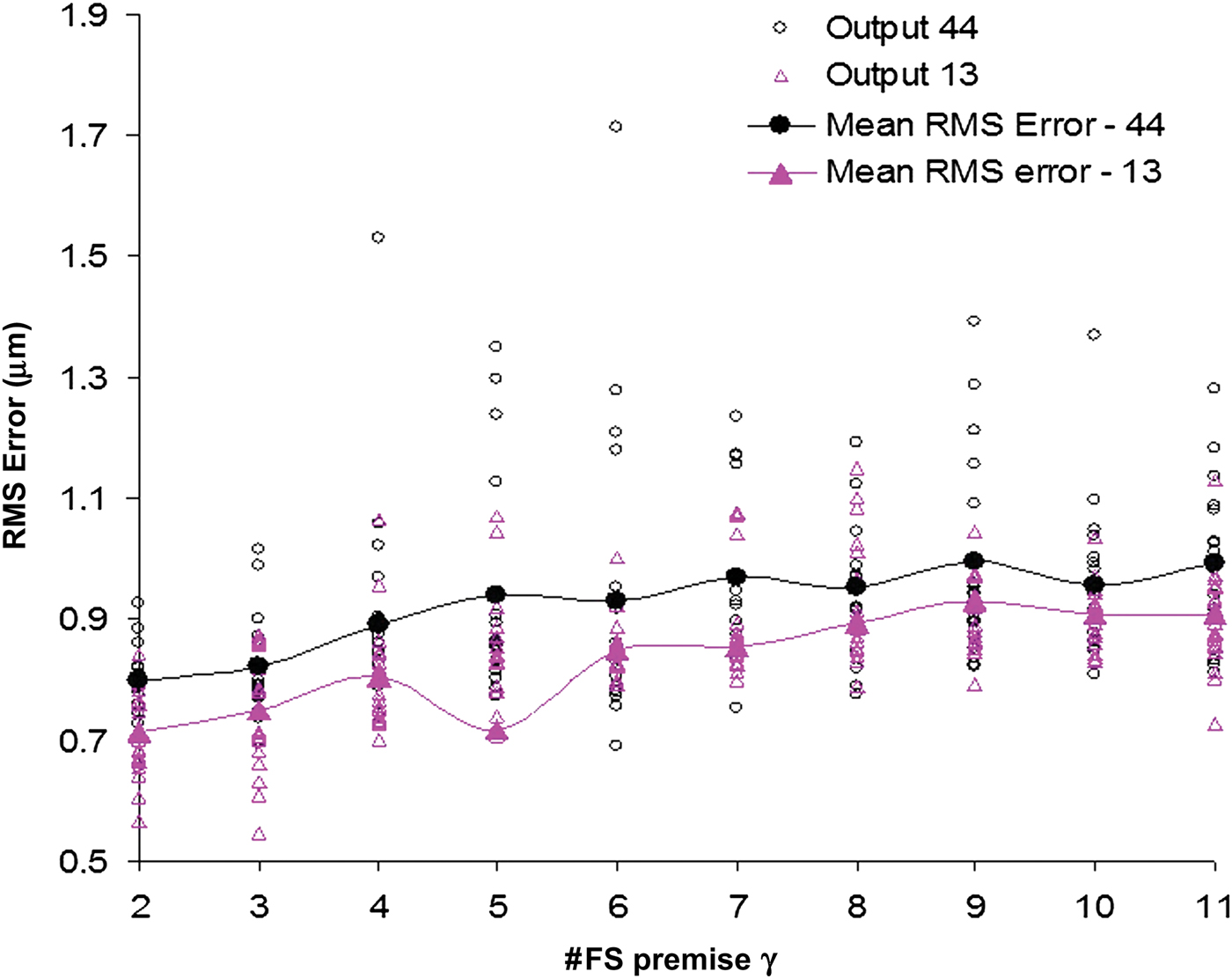
As shown in Figure 10 and Figure 11, the RMS error decreased when fewer FS were used on the conclusion (13 rather than 44). Reducing the number of FS on the conclusion improved the learning by decreasing the size of the FKB and by targeting a more precise set of outputs.

Fig. 10. Root mean square and mean root mean square error versus the number of fuzzy sets on γ (13 vs. 44 fuzzy sets). [A color version of this figure can be viewed online at journals.cambridge.org/aie]

Fig. 11. Root mean square and mean root mean square error versus the number of fuzzy sets on β (13 vs. 44 fuzzy sets). [A color version of this figure can be viewed online at journals.cambridge.org/aie]
Increasing the number of FS on the premises and the conclusion and hence increasing the number of FR did not translate into an improvement of the precision of the automatically generated FKB for this specific task of reconstruction of CMM 3-D triggering probe error characteristics. Furthermore, again from analyzing Figure 7 and Figure 8, one can conclude that the combination of 2 FS on premise γ and 12 FSs on premise β produced a FKB with the lowest error. These two values induce a FR base of 24. In the next section these results will be used to perform near-optimal learning of the FKB.
8.1.2. Optimal learning of FKB for TP6
The learning of a FKB is performed using 2 FS on premise γ and 12 FS on premise β. The best FKB obtained from the learning is illustrated in Figure 12. The number of FS on the output premise was reduced to 7 FS instead of 13. In Figure 12, 13 FS are shown on the conclusion but only 7 are fired by the FRs base, namely, FS: 1, 2, 7, 8 (superimposed with 9), 10, 11 (superimposed with 12), and 13. Hence, FS error outputs for TP6 triggering probe can be semantically labelled as high (FS 13, 12, and 10), medium (FS 7 and 8), and low (FS 1 and 2). In addition, on premise β one can see the 12 triangular FS are actually composed of 8 different summits only, because 11 and 12 are superimposed, whereas 3–2 and 9–8 are straight angled triangles sharing the same physical summit.

Fig. 12. Genetically generated fuzzy knowledge base using an optimized number of fuzzy sets. [A color version of this figure can be viewed online at journals.cambridge.org/aie]

Fig. 13. The profile of the fuzzy predicted error of the TP6 triggering probe. [A color version of this figure can be viewed online at journals.cambridge.org/aie]
The genetically generated FKB reproduces the data with an RMS of 0.58 mm, a maximum absolute error of 2.23 mm, and a minimum absolute error of 0.00 mm. The correlation between the experimental and the predicted error profile is 98.00%.
The FKB illustrated in Figure 12 can be used for CMM calibration to lower the number of setups needed and hence reduce costs in time and money. The positions of the summits of the FSs indicate possible setup values for β and γ angles of the CMM.
Figure 13 illustrates the profile of CMM 3-D triggering probe error characteristics as predicted by the genetically generated FKB. One can see similarities between Figure 3 and Figure 13, however, the genetic-fuzzy predicted profile is smoother and less prone to big local jumps and/or deviations of calibration errors. This can be considered an improvement.
8.1.3. Partial conclusion
Increasing the number of FS on the premises and the conclusion and hence increasing the number of FRs does not always translate into improvement of the precision of an automatically generated FKB. A good balance between these numbers has to be found in order to optimize the automatic learning. Reducing the number of FS on premises γ and β produced a more accurate FKB. Furthermore, the precision of the FKB was more sensitive to increasing the number of FS on premise γ than on premise β; this can be explained because β is measured along the probe axis, which makes it less influential on the errors. The number of FSs on premises γ and β can be used as a number of setups when modeling CMM 3-D triggering probe error characteristics. Furthermore, reducing the number of setups reduces the time required for reconstruction of the compensation model and can also increase its efficiency. The summit of each of the FSs of the inputs can be used as a setup value for future calibrations; in this particular case it means a combination of two setup values for γ and eight for β.
8.2. Modeling TP200 gauge error profile and settings
In this section the FKB equivalent to the 3-D error profile of TP200 is presented. The learning starts with 8 FSs on each premise (γ and β), 8 FS being the highest number of FS obtained for fuzzy modeling of TP6 triggering probe. For the conclusion, a maximum of 13 FSs is used; again, this number is obtained from the TP6 FKB. The RBCGA is allowed to reduce these numbers in order to find a simple near-optimal FKB. The same evolutionary strategy previously used is utilized for TP200 fuzzy reconstruction of the error profile.
The near-optimal genetically generated FKB reproduced the data with an RMS of 0.21 mm, a maximum absolute error of 0.57 mm, and a minimum absolute error of 0.00 mm. The correlation between the experimental and the predicted error profile is around 99.00%. As one can notice from Figure 14, the error profile is smoother and less prone to big local jumps and/or deviations than the experimental calibration error profile (see Fig. 4).

Fig. 14. The profile of the fuzzy predicted errors for TP200. [A color version of this figure can be viewed online at journals.cambridge.org/aie]
The FKB illustrated in Figure 15 has five FS on premise γ and two FS on premise β (both values were reduced from eight). On the output there are 4 FS; however, FS 1 and FS 2 were extremely close in position so they were manually merged by the authors. Hence, FS error outputs for TP200 triggering probe can be semantically labeled as high, medium, and low.

Fig. 15. Genetically generated fuzzy knowledge base for TP200. [A color version of this figure can be viewed online at journals.cambridge.org/aie]
8.2.1. Partial conclusion
The number of FSs on premises γ and β, five and two, respectively, can be used as the number of experimental setups needed to model CMM 3-D triggering probe error characteristics for this type of probe. Furthermore, using the FKB can lead to a better understanding of the relationships between different directions of probing and the error profile. This could be achieved by adding semantics to the FS of the genetically generated FKB.
In the next section the genetically generated FKBs for both TP6 and TP200 triggering probes are analyzed in order to understand the relationships between the setup angles and the pretravel values. This is done through a semantic translation of the FRs bases.
9. ANALYZING THE FRS BASES FOR TP6 AND TP200 FKBS
In order to add to the knowledge about relationships that exist between setup angles of the CMM and probing accuracy, the FRs of the previously generated FKB are thoroughly analyzed.
Table 1 and Table 2 contain the FRs embedded in the FKB generated automatically by RBCGA. The FSs on the output were semantically translated into three different states: low, medium and high. These tables could easily be used by the calibration technician when using TP6 or TP200 because they provide explicit information on the state of the errors depending on the position of the probe.
Table 1. Fuzzy rules for the TP6 error profile

Table 2. Fuzzy rules for the TP200 error profile

From Table 1 one can notice that FSs 7 and 8 along with 11 and 12 on premise b share the same position (same value of the angle). The reason is that they are superimposed and the authors chose to leave them in the FKB. However, they cause no ambiguity because they use the same FR. Furthermore, FSs 2, 3, 7, 8, and 9 are preceded by the sign “<” for inferior to the value or “>” for superior to the value. The reason for this being that the RBCGA proposed right-angled triangles rather than regular ones, which allows use of different FRs around the main value—summit—if needed (however, not the case here).
Table 2 contains the FR for the TP200 FKB. One can notice that error values are high for lower values of γ and low for higher values of γ. This information could help the CMM technician to be aware of the influence of setups on the resulting pretravel values.
10. CONCLUSION
We have presented FKB modeling 3-D triggering probe pretravel. A new method utilizing a low-force high-resolution displacement transducer has been applied and described. This method allowed measurements of a real pretravel length in an XYZ space. A satisfactory agreement of the experimental observations with FKB error predictions has been obtained.
The level of correlation of the probe pretravel with the fuzzy prediction is higher than 98% for two different probes. The FKBs for accuracy profiles were developed for one-stage and two-stage probes.
The influence of the number of FRs on FKB accuracy in reproducing the pretravel was investigated, and the results showed that a lower number of rules and simpler FKB performed better. The number of FSs obtained from this investigation was used as a starting point for optimal FKB learning.
We have assessed which of the setup angles has the highest contribution on the value of the pretravel length. Tilting of the probe holder in the YZ plane of the measuring system has a higher impact on pretravel value. These conclusions were also easy to see from analysis of the FRs bases of genetically generated FKBs. These FKBs offer a better understanding of the influence of the different directions of probing on the error by adding semantics to the FSs. Furthermore, the number of FSs and their position on premises β and γ can be used as the number and positions of setups when modeling CMM 3-D triggering probe error characteristics. Reducing the number of setups reduces the time required for reconstruction of the compensation model and can also increase its efficiency by reducing the risk of human error due to longer manipulation of the measuring devices.
It is worth noting that when the FKBs will be implemented one has to assume that the angular orientation of the probe is known. This can be either determined experimentally or that the probes' producers can determine the angular position of the probe transducer with the special mark.
ACKNOWLEDGMENTS
This work was partially funded by the Homing Grant of the Foundation for Polish Science supported by MF EOG subvention. This work was also partially supported by the Ministry of Science and Higher Education of Poland as the Grant for the research project. The authors thank all the participants of the experiments conducted in this paper.
Sofiane Achiche is a Professor in the Department of Mechanical Engineering, École Polytechnique de Montréal, University of Montreal. He received his PhD in mechanical engineering at the University of Montreal, École Polytechnique de Montréal. His research interests focus upon evolutionary computational intelligence for control and decision support applied to engineering problems such as emotional design, process control, measurements, mechatronic systems, and decision making.
Adam Wozniak is a Professor at the Institute of Metrology and Biomedical Engineering, Faculty of Mechatronics, Warsaw University of Technology, where he teaches and conducts research. From 2005 to 2006 he was a Visiting Professor at École Polytechnique de Montréal. He received his MS and PhD degrees from the Warsaw University of Technology. His current research interests include dimensional metrology, especially coordinate measuring techniques. Dr. Wozniak has published more than 70 papers in these areas.