2. A MODEL OF THE SPUR GEAR TOOTH WITH THE CIRCULAR-ARC FILLET

In the first step, an involute profile is obtained from the first principle as the locus of a point on a tangent line rolling over the base circle without slipping, and the spur gear tooth flank is obtained by rotation of this profile through a half-tooth angle. With the gear center as the origin and the centerline of the tooth as a reference (Fig. 1), polar angle θ_i of a point on the flank at radius R _i is given by

where θ₀ = π/2z and α_i = cos⁻¹(R _b/R _i), z is the number of teeth on the gear, α₀ is the design pressure angle, and R _b represents the base circle radius. The radius R _i is varied from the tip circle to the base circle in an incremental manner (Δr) to construct the complete involute profile. For cases where the root circle is inside the base circle, the profile is further extended by a radial line up to the root circle.

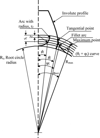
Fig. 1. The arc placed tangential to the involute.

In the next step, a circular arc is placed such that it is tangential to the involute curve as well as the root circle (Subba Rao et al., Reference Subba Rao, Suryanarayana Rao, Shunmugam and Jayaprakash1993). This is done using a computer-aided approach as described below. The arc with a radius (r _f) is divided using the same incremental radius (Δr) as shown in Figure 1, and angles subtended φ_i are calculated using

In the next step, the angle θ_i of the involute profile and corresponding φ_i of arc are added. The maximum angle θ_max is obtained with respect to the tooth centerline as

The radius R _max corresponding to θ_max yields a point at which the arc is tangential to the involute. To establish the circular arc below the tangential point corresponding to R _i, the angle ψ_i is calculated as follows

To compare the proposed fillet with the trochoidal fillet, the tooth flank along with the trochoidal fillet is generated using a basic rack with a tip radius R _c. Analytical equations to arrive at coordinates of points on the trochoidal curve are well documented in the literature (Buckingham, Reference Buckingham1963; Reddy et al., Reference Reddy, Shunmugam and Siva Prasad2004b), and hence, are not included here. It is important to know that the fillet stress is calculated considering the radius of r _f at a critical section, as the radius of the trochoidal curve continuously changes. This specific point is obtained as a contact point between a tangent drawn at an angle of 30° with reference to the centerline of the tooth and the fillet curve (Merrit, 1971). Figure 2 shows the relation between the fillet radius (r _f) and cutter tip radius (R _c), as the number of teeth (z) on the gear varies.

Fig. 2. The relation between the fillet radius (r _f, mm) and the cutter tip radius (R _c, mm); pressure angle (α₀) = 20°, module (m) = 1 mm, addendum (b ₁) = 1.25 m.

A program is written in MATLAB (MathWorks, 2001) to generate the involute flank along with fillet curves for a given number of teeth (z), module (m), pressure angle (α₀), and fillet radius (r _f). Figure 3 shows a comparison of the tooth fillets obtained with the arc of a specified radius and trochoid generated by the corresponding tip radius of the cutter for a different number of teeth.

Fig. 3. A comparison of the fillet curves; pressure angle (α₀) = 20°, module (m) = 1 mm, fillet radius (r _f) = 0.35 mm.

3. EVALUATION OF FILLET STRESS

The ISO code can be used for calculating the fillet stress at a specified point on the trochoidal fillet only. However, the fillet stress can be evaluated by FEM for both models of the tooth (Reddy, Reference Reddy2005).

3.1. FE analysis of the gear tooth

A two-dimensional three-tooth gear model is generated using two-dimensional eight-noded PLANE 82 elements for the profiles obtained with the fillet arc and trochoidal curve, and the stress analysis is done using a general purpose FE program ANSYS (2001). Table 1 indicates the geometric parameters used for the gear tooth geometry and material properties for FEM computations. The rim thickness of the spur gear (t _min) is taken as 5m (von Eiff et al, Reference von Eiff, Hirsch Mann and Lechner1990).

Table 1. Parameters used for gear tooth sector in finite element method computations

Boundary conditions are specified by fixing the sides and inside surface of the gear rim for all degrees of freedom. The FEM model is considered as a plane stress problem with the unit width of the gear teeth. Figure 4 shows the typical FE mesh employed for the analysis. A fine mesh is provided in the fillet area for the profiles obtained by the arc and trochoidal curve. The normal tip load F _na is resolved into a tangential load F _ta using a pressure angle α_an at the tip, as shown in Figure 4. The radial component of the normal tip load is not considered, as the ISO (1996) code neglects the effect of the compressive stress because of the radial component of load. The model is analyzed for the fillet stresses taking the tangential load (F _ta) for a unit tip load (F _na) normal to the involute on the middle tooth. The maximum principal stress (σ₁) at the surface of the root fillet is considered as the fillet stress in the present work, taking the maximum principle stress as a failure criterion in the spur gear design. Convergence study has been carried out on the three-tooth model, and an optimum mesh pattern in the tooth model is obtained.

Fig. 4. The finite element mesh of a three-tooth model.

3.2. Comparison of fillet stresses

Fillet stress values obtained with the fillet arc are compared with the results obtained from the trochoid as the fillet. In addition, a comparison of the FEM results is made with the stresses values obtained using ISO formulae for the calculation of the tooth bending stress. Table 2 shows a comparison of the fillet stresses obtained by ISO formulae and those obtained by the FEM for the arc and trochoid. The table also includes the cutter-tip radius (R _c) with respect to the number of teeth for a fillet radius of 0.35 mm.

Table 2. Comparison of fillet stresses

Pressure angle = 20°, module = 1 mm, face width = 1 mm, tip load = 1 N, fillet radius = 0.35 mm, % error = 100[(2) − (1)]/(2) or 100[(2) − (3)]/(2).

FEM, finite element method.

The ISO (1996) approach uses an approximation that the critical section at the fillet is located at an angle of 30° tangential to the fillet. For calculating the stresses based on ISO, the tip load (F _ta) has to be converted to an equivalent load (F _t) at the reference (pitch) diameter and the fillet radius (r _f) to the corresponding tip radius (R _c) of the cutter. The equation for bending stress also includes the tooth form factor and the stress concentration factor, which can be obtained from the charts or using the formulae given in the ISO standards.

4. TAGUCHI'S METHOD OF EXPERIMENTAL DESIGN

Taguchi's parameter design is an important tool for robust design of high-quality systems. Taguchi's method utilizes special sets of the array called orthogonal arrays to study the entire parameter space with only a small number of experiments. The conclusions obtained from the small number of experiments are valid over the entire experimental region. A number of standard orthogonal arrays tables have been constructed to facilitate the design of the experiments. An appropriate orthogonal array is selected on the basis of a number of factors and levels involved in the experiment. It is a matrix of numbers arranged in rows and columns, where each row represents a level of factors in each run and each column represents a specific factor that can be changed for each run (Park, Reference Park1996).

A selection of factors is more problem specific. In the gear standards, the tip radius of the basic rack is expressed in terms of the module. For the present investigation, the fillet radius is taken as an independent parameter. The stresses developed at the fillet portion are found to vary with the pressure angle, module, fillet radius, and number of teeth. Therefore, these four parameters (pressure angle, module, fillet radius, and number of teeth) are taken as control factors. The values of the normal tip load (F _na) and face width (b) are taken as the unity. For each control factor, five levels having equal spacing are selected, as shown in Table 3. If the traditional experimental procedure is followed with five levels for each variable, a total of 5⁴ = 625 experiments are needed to generate the data set. Instead, by using Taguchi's orthogonal array, the number of data sets gets reduced. However, the results obtained from the small number of experiments are valid over the entire experimental region. A standard Taguchi L₂₅ (5⁶) orthogonal array (Park, Reference Park1996) chosen for the present investigation reduces the number of data sets to 25. Although the chosen orthogonal array consists of six columns at five levels, only four columns are considered for the selected parameters. For all possible combinations of design parameters present in the orthogonal array, the FE simulations are carried out and the fillet stress values obtained are recorded. The results obtained for the given set of parameters may be analyzed further by statistical methods to bring out their contributions. The interpretations thus obtained are valid for the entire experimental region. However, in the present work, the data set generated according to Taguchi's orthogonal matrix (Table 4) are used to train the ANN.

Table 3. Control factors and their levels for Taguchi method

Table 4. Training data set based on Taguchi L25 orthogonal array

FEM, finite element method.

5. ANNs

An ANN is a massively distributed parallel processor consisting of small information processing units, namely artificial neurons (Ham & Kostanic, Reference Ham and Kostanic2001). The artificial neuron is a simple processor, which takes one or more inputs and has a summing up junction and an activation function. Each input into the neuron has an associated synaptic weight that determines the intensity of the input. The summing junction performs the weighted sum of inputs by multiplication of each of the inputs by its respective weight, and produces an output according to an activation function as shown in Figure 5. The output obtained from activation function is multiplied with a specific weight and transferred to the next node. Mathematically, the operation of the artificial neuron can be represented by the following pair of equations.

Fig. 5. The artificial neural network model (Haykin, 2001).

where x ₁, x ₂, … , x _n are the input signals; w _k1, w _k2, … , w _kn are the synaptic weights of neuron k; v _k is the linear combiner output because of the input signals; θ_k is the bias;  f(.) is the activation function; and y _k is the output signal of the neuron. The bias θ_k has the effect of increasing or lowering the net input to the activation function. The output of the neuron is calculated depending on the nature of the activation function. The activation function is also called the squashing function as it squashes the permissible amplitude range of the output signal to some finite value. The sigmoid and tansigmoid are the commonly used activation functions because of their simple derivative, which is useful for the development of the learning algorithm, continuous output data, and simplifying the fundamental mathematics involved in the calculation of individual weights. In the present work, the sigmoid activation function is used and the output of the neuron using the sigmoid function is given as

Among the multilayer network used for modeling a process, the simplest type of network is a three-layer network with one input layer, one hidden layer, and one output layer, as shown in Figure 6. Four input parameters (pressure angle, module, fillet radius, and number of teeth) are considered in the present work, and these are fed to four neurons in the input layer. A single neuron in the output layer is considered to represent maximum stress in the fillet. The number of neurons in the hidden layers is ascertained by trial and error method, because there is no specific rule or procedure for deciding the number of neurons in the hidden layers (Reddy et al., Reference Reddy, Shunmugam and Siva Prasad2004a). After a number of trials with various initial weights and bias, the 4-5-1 configuration is found to be the most suitable network for the present work (Fig. 6). An NN has to adjust its parameters such that the output node produces the given output for a set of given input parameters. The process of adjusting the weights of a network, for a set of given input and output values, is known as the training of the network. The BP algorithm is the most popular and commonly used algorithm for training.

Fig. 6. The neural network model for the prediction of the fillet stresses of the spur gear tooth.

5.1. BP algorithm

The BP algorithm consists of two phases through the different layers of the network, namely, the forward phase and the backward phase, as explained below.

5.1.1. Forward phase

During the forward phase, input vectors in the training set are applied in a feedforward manner and the actual output for the given input training pattern is determined by computing the output of the neuron in the hidden layer. The connection weights are initialized to small random values. The output of every neuron is computed using Eqs. (1) and (3).

5.1.2. Backward phase

The difference between the desired output and the computed output from the output neuron is used to obtain the equivalent error. This error is cumulative and computed over all the training data set. In the backward phase, the error is subsequently backpropagated from the output layer to the hidden layers for an update of weights leading to the neurons in a hidden layer. The process is repeated for the large number of iterations (epochs) until the output error converges to a minimum and optimum sets of the weights are obtained in proportion to the negative gradient of error with respect to the weight. The mean square error (MSE) is used as a way of measuring the best fit to the data:

where P is the number of training patterns in the training data set, K is the number of output nodes, T _pk is the target output for pth pattern of output node k, and O _pk is the computed output for the pth pattern.

The connection weights between the neurons of adjacent layers are modified repeatedly based on the gradient descent optimization criteria to minimize the above squared error. The change in weight is given as

The weight increment is given by the relation

Considering the activation function as sigmoid, the output vector of the NN is calculated. After simplification, the following expressions for error terms are obtained:

for the output nodes and

for the hidden nodes. The weights connecting the neurons in the hidden layer to those in the output layer are adjusted according to

for the output neurons. The weights connecting the neurons in the input layer to those in the hidden layer are adjusted as

for the hidden neurons, where W_kj is the weight connecting neuron j in the hidden layer to the neuron k in the output layer and W_ji is the weight connecting neuron i in the input layer to j in the hidden layer. The second term on the right-hand side of Eqs. (9) and (10) is the learning term, and η is the learning rate parameter, which must be set to a value between 0 and 1. The higher learning rate will generally lead to oscillation around the region of the minima, whereas the low learning rate will result in a slower rate of convergence. Use of the momentum term (third term) ensures quicker convergence without oscillation. The subscript n indexes the presentation number, and 0 ≤ α < 1 is a momentum constant (Yegnanarayana, 1999). The momentum term reduces the effects of the local minima of the error surface and accelerates the gradient descent to the global minimum of the error surface. In the present work, the learning rate parameter η is taken as 0.01 and the momentum constant α as 0.8.

Because the modification of weights proceeds backward from the output to the input, this algorithm is called the BP algorithm. The standard BP algorithm for training of a multilayer feedforward NN is based on the steepest descent algorithm applied to the minimization of the energy function representing the MSE (Rumelhart et al., Reference Rumelhart, Hinton and Williams1986).

For the prediction of the fillet stresses in the gear tooth, the chosen 4-5-1 network is trained using 25 sets of input data and the corresponding stresses obtained by FEM (Table 4). Before training, all the inputs and outputs are normalized with respect to the corresponding maximum and minimum values so that the normalized values lie between 0 and 1. A network training function known as TRAINLM (MathWorks, 2001) that updates weights and bias values in a BP algorithm according to Levenberg–Marquardt optimization is used in the present work.

An MSE of 10⁻⁶ is taken as the desired goal, and the network is trained until the desired accuracy of error is reached. Figure 7 shows the pattern of convergence during the training with the five hidden neurons. After completion of the training, the weights are stored along with the network architecture for further use.

Fig. 7. The convergence characteristics during training of the five hidden neurons.

Finally, the performance of the NN is evaluated with FE simulations of the testing data set and the results are given in Table 5.

Table 5. Testing of neural network with finite element method (FEM) results

% error = 100[(2) − (1)]/(2).

6. RESULTS AND DISCUSSION

In the present work, a circular arc is considered as the fillet for modeling the gear tooth, and a computer-aided approach is described to construct a spur gear tooth from the first principle. In practice, the designer can specify the fillet radius first, without any need for a priori knowledge of manufacturing method. The manufacturer can select later a suitable manufacturing method to arrive at the required geometry. In general, depending on the generation cutting method selected, a suitable cutter geometry with an appropriate tip radius can be chosen to produce a fillet curve with a specified radius at the critical section of the tooth. For a cutter having a geometry as a basic rack profile, a tip radius can be selected from Figure 2. In specific cases, for example, the proposed geometry on cold forging or powder compacting dies can be obtained directly using a wire electro-discharge machine.

Tooth profiles obtained with an arc of a specified radius and a trochoidal fillet generated by a corresponding tip radius of a cutter are shown in Figure 4 for 25, 40, 80, and 100 teeth. A continuous change in the radius of the trochoidal curve from a root circle to a limiting circle can be very well observed for a smaller number of teeth at a higher magnification. On comparing the profiles, it is observed that for a smaller number of teeth, a fillet arc lies inside the trochoid. Although an attempt has been made to get the corresponding fillet radius, the radius obtained is valid only for a specified point at the critical section. The tangency conditions between the involute profile and these two curves are also different. Because of these two reasons, the profiles obtained by the arc of a specified radius and trochoid deviate marginally. With an increase in the number of teeth, the curves tend to merge and the fillet curve obtained with an arc is in good agreement with trochoidal curve for a larger number of teeth.

From Table 2 it can be observed that the FEM values are higher than the corresponding values obtained by the ISO method. This trend is similar to those already published (von Eiff et al., Reference von Eiff, Hirsch Mann and Lechner1990). This may be because of the assumption made in the ISO about the critical point at which maximum stress occurs. Taking the values obtained by the FEM with an arc of a specified radius as a reference, the percentage of error is calculated for the stresses obtained by ISO and FEM with the trochoid. From Table 2 it is observed that percentage of error for a 25-tooth gear is larger, as the fillet arc results in a narrower tooth near the root. As the number of teeth increase, the difference in the magnitude of the fillet stresses obtained for the arc and trochoid reduces to 3%. The percentage of error for the stresses based on the ISO formulae varies from 7 to 19%.

The present investigation is done with four parameters at five levels using the Taguchi orthogonal array L₂₅ (5⁶). Although the number of training data gets reduced to 25, the results obtained from such a small number of experiments are valid over the entire experimental region. To ascertain whether the trained NN is exhibiting good generalization capability, a set of 30 test data other than the training set is taken, fed to the trained NN, and the fillet stresses are obtained as the output. For the test set, the fillet stress values are also obtained by the FE simulation. Comparison of the results of the NN and FEM are shown in Table 5. It can be observed that the difference between the values predicted by NN and FEM varies from −3.123 to 5.144%, and for 25 out of 30 test data values the error is within 3%. The average absolute deviation of the testing data set from FEM simulations is 1.849%. This establishes confidence in the predictive capabilities of the NN model.

Although statistical methods are available for the development of an empirical relationship between the various interacting factors, these are often complex and circuitous, particularly for nonlinear relationships. There is no need to specify a mathematical relationship between the input and output variables if ANN modeling is used. In the FE approach, each case takes around 30 min for the tooth modeling, meshing, and analysis. Even though the training of the NN takes about 14.5 h (12.5 h for the FE analysis of the 25 training sets and 2 h for the training), it is able to predict the fillet stresses within 0.03 s for each case. Once trained, the NN is able to predict the fillet stresses with reasonable accuracy and faster than the FEM simulations. Therefore, the proposed ANN approach can be used for routine and repetitive applications for the prediction of fillet stress in the spur gears having 25–125 teeth, a 1–5 mm module, a 0.05–0.45 mm fillet radius, and a 15°–25° pressure angle. For critical applications, the gear parameters selected on the basis of stress predicted by the ANN can be confirmed by FEM simulation. The results thus obtained can be used in addition to train the network, and the prediction accuracy would improve when more such data sets are available with time.