


Introduction
Rapid prototyping is used to quickly fabricate a scale model of new products to examine its shape, size, fitment, working mechanism, and other operational and aesthetic features. The fitment and working mechanism of the prototypes confirms the design features of the new products before initiating the production schedules. Prior to rapid prototyping, the prototypes were formed using traditional manufacturing processes, namely casting, machining, welding, etc. However, these traditional techniques were time-consuming and expensive. Therefore, rapid prototypying was evolved as a new technology to make prototypes, in which a physical part or assembly is fabricated using additive manufacturing or 3D printing. In 3D printing, the product is made by adding a layer on another layer and the final product is obtained by continuously repeating this layer addition (Narang and Chhabra, Reference Narang and Chhabra2017). The products are directly obtained according to the three-dimensional computer model generated from aided design (CAD) software supplied to the 3D printer. The applications of 3D printing process is increasing exponentially in the field of product prototyping due to less involvement of post processing. Similar to the prototype making, different decorative structures, human body parts, and many end-use products are also manufactured using 3D printing. Even some researchers are using this technology for manufacturing their experimental setup and its parts with the desired configuration (Yadav and Kumar, Reference Yadav and Kumar2021a, Reference Yadav and Kumar2021b). Such applications increase the scope of 3D printing in automotive, medical, electronics, and research sectors.
After subsequent development, the technologies under 3D printing are categorized based on their working process and raw material used. The technologies namely stereolithography, fused deposition modeling (FDM), drop on demand, 3DP, and laminated object manufacturing are based on processes such as vatpolymerization, material extrusion, material jetting, binder jetting, and sheet lamination, respectively. These techniques are dedicated for processing polymers like Acrylonitrile butadiene styrene (ABS), polylactic acid (PLA), Polyethylene terephthalate glycol (PETG), etc. (Wimpenny et al., Reference Wimpenny, Pandey and Jyothish Kumar2016; Gibson et al., Reference Gibson, Rosen, Stucker and Khorasani2020; Brennan et al., Reference Brennan, Keist and Palmer2021; Singh et al., Reference Singh, Missiaen, Bouvard and Chaix2021). To process metals and their alloys, powder-based fusion (PBF) and directed energy deposition (DED) methods are being used. The PBF-based techniques such as selective laser sintering and direct metal laser sintering are focused to process the materials in powder form, whereas techniques under the DED process, namely wire arc additive manufacturing (WAAM) and electron beam additive manufacturing (EBAM), are dedicated to raw material in wire form (Liu and Shin, Reference Liu and Shin2019; Hafenecker et al., Reference Hafenecker, Papke and Merklein2021). With the wide coverage of manufacturing aspects, 3D printing becomes the emerging area of research and the choice of industries.
Among all 3D printing technologies, the FDM process is widely used because of low initial installation and maintenance cost. The FDM process involves the basic principle of melting, extruding, and solidifying thermoplastic material in a predefined shape. The extrusion system regulates melt flow by forcing raw material through a nozzle in a heated chamber and extruded material solidifies due to the heat loss phenomenon (Sharifabad et al., Reference Sharifabad, Derazkola, Esfandyar, Elyasi and Khodabakhshi2021). The performance of FDM produced parts affected by controllable parameters, namely infill pattern, number of shells, fan speed, infill density, layer thickness, printing speed, outer cell speed, part bed temperature, shell thickness, etc., as shown in Figure 1. As the FDM process involves material deposition in layer upon another layer manner, this leads to staircase effect in the final product; hence, it increases SR. SR is the deviation in normal to the printing plane from the desired surface. In prototype and decorative structures, the SR and dimensional accuracy are the crucial requirements for the final product. Whereas the dimensional accuracy refers to how closely the dimensions of the fabricated object match to those of the CAD model. The SR of FDM-produced components can be minimized either by the optimization of effective input process parameters or by employing post-treatments. But post-treatments involve either the addition of one layer on the surface or removal of one existing layer from the surface which may cause inaccuracy in dimensions.

Fig. 1. FDM (a) process model and (b) controllable input parameters.
The optimization process begins with the generation of a large number of experiments by varying the combination of input variables (Thakur et al. Reference Thakur, Guleria and Lal2022). The experimental plan can be designed by using different methods under CCD and Taguchi method. But the Taguchi method is a reliable statistical tool for designing experiments and optimizing processes with less experiments (Guleria et al. Reference Guleria, Kumar and Singh2022a). This methods employs a special set of arrays known as orthogonal arrays, which explain how to run the fewest number of tests possible while obtaining complete information on all aspects that influence performance parameters (Mitra et al., Reference Mitra, Jawarkar, Soni and Kiranchand2016). After getting output responses, mathematical modeling and artificial techniques help in building the relation between input and output parameters. Artificial intelligence (AI) techniques such as artificiail neural network (ANN), Particle Swarm Optimization (PSO), whale optimization algorithm (WOA), and their hybirdization perfom better than the optimization of conventional methods.
The ANN model is a robust nonlinear modeling approach for prediction that uses allotted weights and activation functions to promote the creation of linkages between input and output variables (Vaheddoost et al., Reference Vaheddoost, Guan and Mohammadi2020). This model helps in discovering the implicit relationship in the problem-solving process to obtain the result. For this reason, a large amount of data is employed in the training stage, followed by the calculation of the right output using the relationship discovered in the previous step (Samadianfard et al., Reference Samadianfard, Hashemi, Kargar, Izadyar, Mostafaeipour, Mosavi, Nabipour and Shamshirband2020). Another AI technique is WOA to address optimization issues using an evolutionary strategy (Mirjalili and Lewis, Reference Mirjalili and Lewis2016). The humpback whales’ bubble-net feeding pattern inspired the WOA algorithm's hypothesis.
The researchers are employing optimization techniques such as Response Surface Methodology (RSM) and AI algorithms to the input parameters of FDM process for getting a low SR. In this context, some researchers implemented hybrid ANN and PSO to optimize the input parameters such as printing speed, printing temperature, and outer cell speed which result in the minimal SR of PLA material components (Saad et al., Reference Saad, Nor, Baharudin, Zakaria and Aiman2019; Shirmohammadi et al., Reference Shirmohammadi, Goushchi and Keshtiban2021). Radhwan observed that the effect on SR of the PLA printed is components directly effected by nozzle temperature, filling density, pattern style, layer thickness, and printing speed nozzle diameter (Radhwan et al., Reference Radhwan, Shayfull, Farizuan, Effendi and Irfan2019). While in case of Polycarbonate (PC), SR is directly affected by layer height and inversely proportional to print speed and build angle (Hartcher-O'Brien et al., Reference Hartcher-O'Brien, Evers and Tempelman2019). Whereas the SR of copper–PEG composite printed parts is directly proportional to layer thickness and nozzle temperature (Singh et al., Reference Singh, Missiaen, Bouvard and Chaix2021). The SR of ABS components was increased remarkable by utilizing vaproized acetone 1500 mm3 (Kesvarakul and Limpadapun, Reference Kesvarakul and Limpadapun2019). In continuation, the effect of process parameters on the SR, production time (PT), and build volume of printed products are tabulated in Table 1. Some of the researchers have implemented AI algorithms in different research areas for various applications (Chauhan and Vashishtha, Reference Chauhan and Vashishtha2021; Chauhan et al., Reference Chauhan, Singh and Singh2021; Vashishtha and Kumar, Reference Vashishtha and Kumar2021a, Reference Vashishtha and Kumar2021b, Reference Vashishtha and Kumar2022; Vashishtha et al., Reference Vashishtha, Chauhan, Singh and Kumar2021 Guleria et al. Reference Guleria, Kumar and Singh2022b).
Table 1. Literature studied on the impact of input variables on the SR of FDM-fabricated product

From the literature review, it is evident that researchers have worked extensively for the improvement of SR of PLA components by the optimization of input parameters of FDM printer. But very less work has been carried in the optmization of the process parameters for the combinations of outcomes such as SR, dimensional accuracy, and PT. Also very less work has been reported in the implementation of hybrid algorithm for such desired outcomes.
Taking previous studies into account, the present work is aimed to study the parameters of 3D printing for optimizing input parameters, namely layer thickness, nozzle temperature, printing speed, and raster width of FDM process for minmizing SR, PT, and volume percentage error (VPE). In this paper, a newly developed hybrid ANN–WOA model has been employed for fixing up the input variables. The optical micrographs have been taken to study the impact of input parameters on SR.
Research methodology
This paper attempts to propose optimized input parameters for the FDM process which are aimed to prepare PLA components with low SR, PT, and VPE to meet the demand of rapid prototyping. The research methodology followed in accomplishing the present research work consisted of the various aspects such as literature review, the identification of the objective of the research issue, designing experimental matrix using the Taguchi method L27 orthogonal array (OA), preparing samples as per research plan, testing of samples, the optimization of input parameters for minimizing the output response using hybrid algorithms, study outresponse, and deriving conclusion. Figure 2 illustrates the research methodology steps performed in concluding the research work.

Fig. 2. Flow chart of the methodology adopted.
Experimental design
In this study, the Taguchi design of the experimental method has been employed to establish the relative importance of process parameters on outcomes of the FDM process such as SR, VPE, and the PT. In this study, the L27 orthogonal array has been created by varying input variables within their ranges and is tabulated in Table 2.
Table 2. Process variables and their levels

The input parameters, namely layer thickness, nozzle temperature, printing speed, and raster width of the FDM process, have been considered in the present research with three levels and three output responses calculated as shown in Table 3. White PLA, a biodegradable material, has been used for 3D FDM printing due to its fast prototyping, ease of printing, and cost-effectiveness.
Table 3. Input parameters and output responses

Product modelling and testing
The 3D model of the samples has been developed in CATIA V5 software. The slicing of the model, setup of printing parameters according to the Taguchi design of experiments, and the calculation of the tool path have been performed in Cura 4.5 software. The toolpath with set parameters has been transferred to the Ultimaker S5 (300 × 250 × 320 mm3) 3D printer using a flash drive through the USB port. The flow process of 3D design to final printing has been depicted in Figure 3. The response parameters such as SR, dimensional accuracy, and time are taken to build the specimen, which have been measured after the completion of 3D printing using a contact-type SR tester (Talysurf model), digital vernier calliper (Mitutoyo), and digital stopwatch, respectively, as shown in Figure 5a. The average of three observations is considered for dimension measurement and SR on the front (face A), side (face B), and top (face C) surfaces as shown in Figure 4b. The ANN prediction models with Levenberg–Marquardt have been developed. The objective functions obtained from the models have been optimized using the whale optimizaton algorithm. The validation of these optimized parameters has been done by comparing them with experimental values (Figure 5).

Fig. 3. Flow process.

Fig. 4. (a) FDM-printed specimen and (b) SR tested on face A, face B, and face C.

Fig. 5. (a) SR test (Talysurf model) and (b) digital vernier calliper (Mitutoyo) for dimension measurement.
AI algorithms
The relationships have been developed between input parameters and output response using ANNs and WOA. The hybrid algorithm ANN–WOA is used for the optimization of output response.
Artificial neural network
In this research, MATLAB version 2019b has been utilized to construct and prepare a self-learning model, that is, feed-forward backpropagation neural network which involves the range of activation functions, large numbers of neurons, and hidden layers. The parameters of the model have been optimized using a multi-layered feed-forward perceptron technique. In the training stage – Levenberg–Marquardt (LM) back-propagation method in the hidden and output layers – tangent and linear transfer functions were utilized. As a result, the Hessian and Jacobian matrix have been obtained.
 $$H = J^TJ$$
where H and J are Hessian and Jacobian matrix, and J contains the errors.
 $$J = \left[{\matrix{ {\displaystyle{{\partial e_{1, 1}} \over {\partial w_1}}} \hfill & {\displaystyle{{\partial e_{1, 1}} \over {\partial w_2}}} \hfill & \ldots \hfill & {\displaystyle{{\partial e_{1, 1}} \over {\partial w_n}}} \hfill \cr {\displaystyle{{\partial e_{1, 2}} \over {\partial w_1}}} \hfill & {\displaystyle{{\partial e_{1, 2}} \over {\partial w_2}}} \hfill & \ldots \hfill & {\displaystyle{{\partial e_{1, 2}} \over {\partial w_n}}} \hfill \cr \ldots \hfill & \ldots \hfill & \ldots \hfill & \ldots \hfill \cr {\displaystyle{{\partial e_{1, m}} \over {\partial w_1}}} \hfill & {\displaystyle{{\partial e_{1, m}} \over {\partial w_2}}} \hfill & \ldots \hfill & {\displaystyle{{\partial e_{1, m}} \over {\partial w_n}}} \hfill \cr \ldots \hfill & \ldots \hfill & \ldots \hfill & \ldots \hfill \cr {\displaystyle{{\partial e_{\,p, 1}} \over {\partial w_1}}} \hfill & {\displaystyle{{\partial e_{\,p, m}} \over {\partial w_2}}} \hfill & \ldots \hfill & {\displaystyle{{\partial e_{\,p, 1}} \over {\partial w_n}}} \hfill \cr {\displaystyle{{\partial e_{\,p, 2}} \over {\partial w_1}}} \hfill & {\displaystyle{{\partial e_{\,p, 2}} \over {\partial w_2}}} \hfill & \ldots \hfill & {\displaystyle{{\partial e_{\,p, 2}} \over {\partial w_n}}} \hfill \cr \ldots \hfill & \ldots \hfill & \ldots \hfill & \ldots \hfill \cr {\displaystyle{{\partial e_{\,p, m}} \over {\partial w_1}}} \hfill & {\displaystyle{{\partial e_{\,p, m}} \over {\partial w_2}}} \hfill & \ldots \hfill & {\displaystyle{{\partial e_{\,p, m}} \over {\partial w_n}}} \hfill \cr } } \right]$$
-
p = pattern index, ranging 1–p
-
m = output index, ranging 1–m,
-
i and j = weight indices, ranging 1–n, where n refers to the total number of weights.
The entries of the Jacobian matrix are calculated by the following equation:
 $$\displaystyle{{\partial e_{\,p, m}} \over {\partial w_{{\,j, i}}}} = {-}\delta _{m, {\rm j}}y_{{\rm j, i}}$$
where δ is the parameter for neuron j and output m, y ji is the output, i is the ith input node of neuron j, wji is the bias weight of neuron j (Yu and Wilamowski, Reference Yu and Wilamowski2011).
For rapid convergence to minimum mean square error (MSE), all the input parameters were normalized (−1 to 1) by using Eq. (4):
 $$Y_n = 2\displaystyle{{Y_r-Y_{r{\rm \;min}}} \over {Y_{r{\rm \;max}}-Y_{r{\rm \;min}}}}-1$$
where Y n, Y r, Y r min, and Y r max are normalized, raw, minimum, and maximum values of input parameters, respectively (Taghavifar and Mardani, Reference Taghavifar and Mardani2014). The developed ANN model was tested for the minimal MSE and large regression value (R L) to obtain the optimal model.
 $${\rm MSE} = \displaystyle{1 \over N}\Sigma ( X_a-X_b) ^2$$
 $$R_{\rm L} = 1-\displaystyle{{\Sigma {( X_a-X_b) }^2} \over {\Sigma {( X_a-X_m) }^2}}$$
where N is the total experiment, and X a, X b, and X m are experimental, predicted, and mean values, respectively.
Whale optimization algorithm
Inspiration
Whales are magnificent animals. They are regarded as the world's largest animals. An adult whale may have up to a length of 30 m and a weight of 180 tonnes. Whales are fascinating animals because they are thought to be very intelligent and emotional.
By blowing bubbles around the rings, the Humpback Whales seek little fish and other aquatic organisms. By swimming around prey in a decreasing circle, they produce characteristic bubbles along a spiral-shaped pathway as shown in Figure 6. The prey is the target in the WOA algorithm and the likely position of whales near the prey. There are two phases to the WOA. The first is exploitation, which involves encircling the target and employing the bubble spiral assault tactic. Prey are chosen at random in the second stage, which is referred to as exploration (Mafarja and Mirjalili, Reference Mafarja and Mirjalili2018).

Fig. 6. Humpback whales spiral path and updating position.
Encircling prey
Whales trace the position of prey (best solution) and surround it. The whale thinks that the present best solution is the target prey or is near to it. Since the next location of prey cannot be predicted by whale. Therefore, the other prey update their position to the optimal location. This conduct is explained as follows:
 $$\vec{D} = \vert {\vec{C}\cdot \vec{X}( t ) -\vec{X}( t ) } \vert $$
 $$\vec{X}( {t + 1} ) = ( {\vec{{X}^{\rm \ast }}} ) ( {\vec{t}} ) -\vec{A}\cdot \vec{D}$$
where t is the present iteration, C and A are coefficient vectors, X is the location vector, and X* denotes the best solution achieved. A and C are calculated by the following equations:
 $$\vec{A} = 2\vec{a}\cdot \vec{r}-\vec{a}$$
 $$\vec{C} = 2\cdot \vec{r}$$
In the exploration and exploitation stages, a lowered from 2 to 0 throughout iterations, r is the arbitrary vector in between 0 to 1. In the WOA, a is lowered using the following formula to achieve diminishing encircling behavior in a trap:
 $$a = a-t{\rm \;}2/( {{\rm Max}-{\rm itr}} ) $$
where t is a recurring integer and Max-itr is the maximum number of iterations that can be done.
Exploitation phase
To replicate the spiral-shaped search, the gap between the most well-known searches (X*) and a search factor (X) is determined as:
 $$\vec{X}( {t + 1} ) = \overrightarrow {{D}^{\prime}} \cdot e^{bl}\cdot \cos ( {2\pi l} ) + \overrightarrow {X^{\rm \ast }} ( t ) $$
where l is the arbitrary integer [−1,1], b is constant, and ith is the place of whale, and the D ′ is prey (best solution), which are determined as follows:
 $${D}^{\prime} = \vert {\overrightarrow {X^{\rm \ast }} ( t ) -{\rm \;}\vec{X}( t ) } \vert $$
Whales swim in a spiral pattern to target their prey. The chance of the selection among spiral mode and shrinking toward the circle point by the whale has 50% and this behavior is represented by:
 $$\vec{X}( {t + 1} ) = \left\{{\matrix{ {{\rm Eqn}\;( {11} ) } \hfill & {\;{\rm if}\;p < 0.5} \hfill \cr {{\rm Eqn}\;( {12} ) } \hfill & {{\rm if}\;p > 0.5\;} \hfill \cr } } \right.$$
where p is the arbitrary number and its value is in between 0 and 1.
Exploration phase
Instead of requiring solutions to search randomly depending on the location of the prey identified so far, a randomly picked solution is utilized to revise the location in the WOA to improve exploration. As a result, a vector A with arbitrary values > 1 or < 1 is used to compel a solution to depart from the best-known search agent. The mathematical model is as follows:
 $$\vec{D} = \vert {\vec{C}\cdot \overrightarrow {X_{{\rm rand}}} -\vec{X}} \vert $$
 $$\vec{X}( {t + 1} ) = \overrightarrow {X_{{\rm rand}}} -\vec{A}\cdot \vec{D}$$
where  $\overrightarrow {X_{{\rm rand}}}$ is a arbitrary location vector (a arbitrary whale) selected from the current population.
ANN–WOA hybrid model
The block diagram describes the hybrid ANN–WOA algorithm as shown in Figure 7.
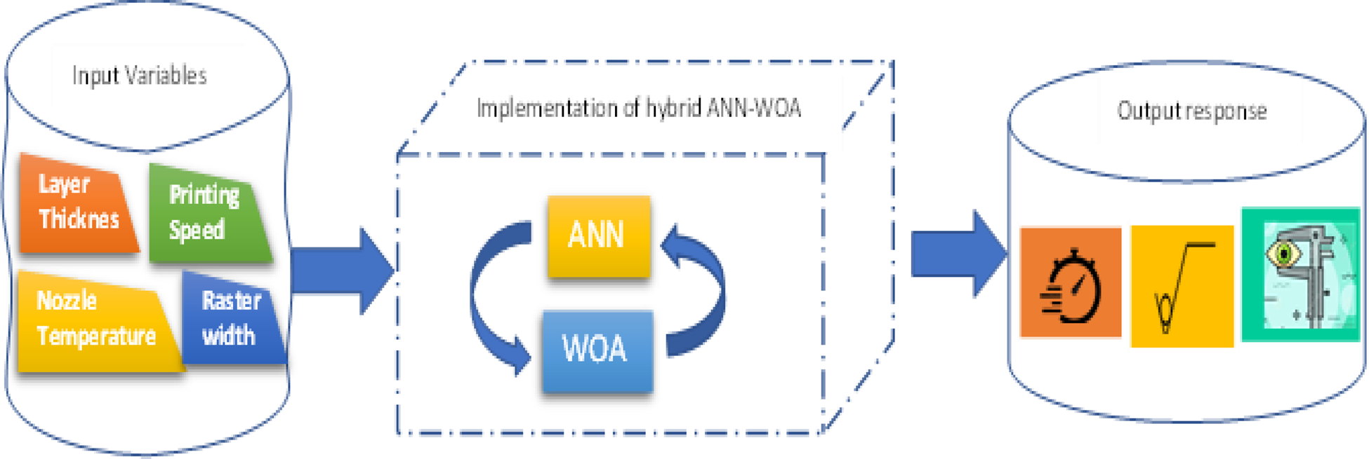
Fig. 7. Hybrid ANN and WOA algorithm.
Results and discussion
The SR, PT, and VPE has been tested for each specimen as per the planned experimental design Taguchi L27 OA. The input parameters and output responses have been tabulated in Table 3.
Analysis of variance
To analyze the significance and fitness of the established model, analysis of variance (ANOVA) is used (Liu et al., Reference Liu, Liu, Li and Meehan2014). The influence of the input factors on the output response, namely SR of face A, face B, and face C, PT, and VPE, which are investigated using ANOVA with 95% confidence level, has been depicted in Tables A.1–A.8 (appendix A). The quadratic model has been developed for all the responses. The significance of the parameters evaluated by the (P-value) probability value (Liu et al., Reference Liu, Liu, Li and Meehan2014). The parameters’ corresponding P-values <0.05 are significant. The predicted value of R 2 has been utilized to assess the established model's ability to predict. The difference between predicted and adjusted R 2 values should be below 0.20 to ensure a satisfactory agreement.
From Table A.1 (appendix A), ANOVA for SR of face A shows that process parameters such as layer thickness, nozzle temperature, printing speed, and their square terms are significant, whereas raster width and its square term are insignificant because raster is infill of the product. For face B refer to Table A.2 (appendix A), the parameters such as layer thickness, nozzle temperature, raster width, and their square terms are significant, whereas printing speed and its square terms become insignificant. Referring to Table A.3 (appendix A) for face C, all considered parameters and their square terms are significant. It implies that all the terms affect the SR of face C. The influence of process parameters on responses has been discussed using optical micrographs in the section “Effect of process parameters on SR”.
ANOVA for PT refers to Table A.5 (appendix A), and all the considered parameters and their square terms are significant. It means that PT depends on process parameters, namely layer thickness, nozzle temperature, printing speed, and raster width.
From Table A.6 (appendix A), ANOVA for VPE depicts that nozzle temperature, printing speed, raster width, and their square terms are significant. The input parameter layer thickness is significant, whereas its square term is insignificant. The regression equations of the all the output response are listed in appendix A from Eqs (A1)–(A5).
Effect of process parameters on SR
The normal probability plot of residuals follows the straight line which shows its uniform distribution, as depicted in Figure 8a–c. The effect of process parameters on response has been studied through main effect plots, as shown in Figure 8d–f.

Fig. 8. Normal probability plot for SR of (a) face A, (b) face B, (c) face C, and the main effect plot for SR of (d) face A, (e) face B, and (f) face C.
From the main effect plot, layer thickness has a direct impact on the SR on all three faces, namely face A, face B, and face C. Because thick layers contribute a large staircase effect, hence surface roughness increases. The effect of nozzle temperature on the surface roughness of all three faces is studied through Figure 8d–f. Figure 8d depicts that SR decreases on increasing the nozzle temperature because at low temperature layers did not get diffuse to each other, hence rough surface obtained at low nozzle temperature. But from Figure 8f, SR first increases as increase in nozzle temperature then decreases as further increase in temperature because at final printing of layers nozzle temperature reduces its temperature from the set value. The effect of printing speed on surface roughness of face A has been seen from Figure 8d that the on increasing printing speed, the SR decreases, and the reverse effect has been seen in case of face C (Figure 8f). Raster width does affect the surface rougness of face A, but it affect the SR of face B and face C.
Study of SR through optical micrographs
To study the correlation between SR and input variables, the optical microscopic images have been taken of specimens as shown in Figure 9. For studying the SR behavior of face A, micrographs of two runs have been chosen for further study, run 2 and run 26, where the SR (Ra) value is best and worst, respectively. At run 2, the SR (Ra) value is least (means best) because layer thickness is minimum and nozzle temperature is high. Due to the high temperature of the nozzle, the layer got mixed into each other. Moreover, at run 26, the SR (Ra) is higher (means worst) due to a higher level of layer thickness and low nozzle temperature, which cause not proper diffusion of layers into each other. Input parameters, namely printing speed and raster width, have an insignificant impact on SR.

Fig. 9. Optical micrographs of specimen for face A (a) run 2 and (b) run 26, face B at (c) run 8 and (d) at run 25, and face C at (f) run 17 and (g) run 22.
For face B, run 4 and run 25 are considered where the SR (Ra) values are best and worst, respectively. Layer thickness, nozzle temperature, print speed, and raster width at run 4 were 0.06 mm, 200°C, 70 mm/s2, and 0.35, whereas at run 25 they were was 0.15 mm, 190°C, 90 mm/s2, and 0.42 mm, respectively. That shows that at lower layer thickness, the SR would be best and at higher it would be worst. In addition to that at higher nozzle temperature, layers got diffused into each other and a better surface finish was obtained.
Further, while studying the SR of face C, there is no such difference in the value of SR in low and high. The little difference is due to the difference in raster width.
Volume percentage error
The VPE of the 3D-printed samples is tabulated in Table 3. Dimensions are measured through a digital vernier calliper and compared with the CAD dimensions. From Figure 10, it has been seen that on increasing the temperature and layer thickness, the VPE increases because high layer thickness leads to dimensional inaccuracy and high temperature causes atoricous product. On increasing print speed, VPE increases then decreases at a higher value. Jayanth et al. (Reference Jayanth, Senthil and Prakash2018) observed the same behavior. High deviation in the middle value raster width has been observed.

Fig. 10. Main effect plot for VPE.
Production time
In 3D printing of the specimens, from Figure 11, it can be seen that layer thickness has a major influence on PT; on increasing the layer thickness, the PT decreases exponentially due to high deposition of material on large thickness, resulting in decreasing the PT. Nozzle temperature does not exhibit significant effect on PT. On increasing printing speed, the PT decreases because fast speed reduces the time to production. Dimensions are measured through a digital vernier calliper and compared with the CAD dimensions. Whereas at low and middle levels of raster width, no significant effect on the PT has been observed but as raster width increases then slightly decreases in PT reported.

Fig. 11. Main effect plot for PT.
Hybrid WOA and ANN analysis
The input process parameter matrix of order 27 × 4 and output response matrix of order 27 × 5 have been retrieved from Table 2. These matrices have been used for training, testing, and validation of the ANN model. The ANN predicted output responses have been tabulated (Table 4).
Table 4. ANN predicted output response

The regression values obtained through the trial-and-error procedure with 10 hidden layers using feed-forward and LM backpropagation algorithm are 0.992 for training point, 0.99311 for validation, 0.9949 for testing, and 0.99734 overall as shown in Figure 12a, b, and d, respectively.

Fig. 12. Regression curves of (a) training, (b) testing, (c) validation, (d) overall, (e) histogram, (f) MSE curve, and (g) gradient, mu and validation check curve.
From Figure 12g, the gradient function in backpropagation descent at epoch 6 with the value of 2.1031×10⁻¹⁴ minimize the function in iterative manner by updating parameters such as weight and bias. And mu is the momentum update having a value of 1×10⁻⁹ at epoch 6. It is included to parameter with updated weight, which helps the gradient descent to avoid the problem of minima that may affect the convergence error. The validation check is used to end the learning of model and its value to define the number of successive trials for iterations.
The best validation performance has been obtained at the 6th iteration with a minimum MSE of 0.15376 as shown in Figure 12e. An error histogram of 20 runs has been plotted between the target (experimental) and predicted output values as shown in Figure 12f, which depicts the error ranges from −1.369 to 1.173.
The developed ANN model has been saved as net.mat file and loaded into the WOA fitness function for optimization. The values of p in this study were 0.65 and 0.37, respectively. In addition, the population size was limited to 30, with a maximum iteration of 1000. The optimal input factors have been found to minimize the SR, time taken, and VPE. The convergence of objective function with respect to the number of generations has been depicted in Figure 13. The minimum value of objective function is obtained at optimized input variable, that is, layer thickness 0.06 mm, nozzle temperature 205.9933°C, printing speed of 90 m/s, and raster width 0.49 mm.

Fig. 13. Convergence behaviour plot.
Validation test
A validation test has been performed on the optimized parameter suggested by the hybrid ANN–WOA algorithm. Three specimens have been prepared on the suggested parameters and their average test results are tabulated in Table 5. The hybrid algorithm's results at predicted parameters are very close to the experimental results.
Table 5. Validiation test

Conclusion
The L27 orthogonal array was utilized to correlate between input variables and output parameters, such as SR, PT, and VPE, for the FDM-processed PLA, and the following are the findings:
1. The layer thickness and nozzle temperature have the greatest effect on SR. The maximum SR obtains at thick layers, but surface roughness minimum at low nozzle temperature. When compared to layer thickness, raster width has less effect on surface roughness.
2. For face A, minimum SR, that is, 4.75 μm, has been obtained using input variables – layer thickness of 0.06 mm, nozzle temperature at 210°C, print speed of 50 mm/s2, and raster width of 0.35 mm.
3. On face B, the minimum SR value, that is, 2.75 μm, has been observed when input parameters – layer thickness, nozzle temperature, print speed, and raster width – are 0.06 mm, 190°C, 90 mm/s2, and 0.49 mm, respectively.
4. The minimum SR of face C has been observed 1.75 μm at input parameters – layer thickness, nozzle temperature, print speed, and raster width are 0.1 mm, 190°C, 50 mm/s2, and 0.42 mm, respectively.
5. While 3D printing of 1000 mm3 cube shape, PT reduces to 6 min and 57 s on increasing the layer thickness, print speed, and nozzle temperature to high levels.
6. The VPE in fabricating the cube of 10 mm dimension reaches to 2% on lowering the layer thickness and nozzle temperature to 0.1 mm and 190°C, respectively.
7. The performance of ANN prediction model increased when hybridized with WOA, as it involves exploration/exploitation for searching best solution.
8. The significant input factors have been successfully modeled using AI algorithms such as WOA and ANN, and results are verified through validation tests. The minimum SR of face A – 4.8 μm, face B – 4.9 μm, and face C – 1.95 μm, PT 15.75 min, and VPE 2 (%) are obtained at optimized input variables.
Supplementary material
The supplementary material for this article can be found at https://doi.org/10.1017/S0890060422000142.
Funding
The work done under this research did not get any financial grant.
Mr. Praveen Kumar is a Research Scholar in Mechanical Engineering Department at Sant Longowal Institute of Engg & Tech Longowal, Punjab, India. He obtained his B.E. and M.Tech. from MDU Rohtak. His research interest includes additive manufacturing, polymer composites and optimization techniques. His research topic during PhD is FDM process optimization for blends. He has 09 years of teaching and research experience.
Dr. Pardeep Gupta is a Professor in Mechanical Engineering Department at Sant Longowal Institute of Engg & Tech Longowal, Punjab, India. He obtained his B.E. and M.E. from PEC, Chandigarh in 1989 & 1997 respectively and Ph.D. degree from NIT, Kurukshetra in 2004. His research areas of interest include Quality and Reliability engineering, TQM, TPM, Industrial Engineering, Conventional and Non-Conventional Metal Machining and Optimization Techniques. He has published more than 80 research papers in various national and international journals of repute and conference proceedings. He has more than 30 years of teaching and research experience.
Dr. Indraj Singh awarded B.E in Mechanical Engineering from Dayal Bagh Education Institute, Agra and M.Tech from PTU, Jalandhar with silver medal. He Earned his Ph.D. from SLIET, Longowal, (A CFTI, Deemed University). He has been working as Associate Professor in the Department of Mechanical Engineering, at Sant Longowal Institute of Engineering and Technology Longowal Sangrur, Punjab since 1997. He has published more than 30 research articles in Journals and National/International Conferences. Dr. Singh has visited Osaka Japan, and two times UK and presented research articles in Imperial college. He has guided more than 17 M.Tech and guiding 2 Ph.D. He has completed two projects of value 18 lacs. He is members of many professional societies e.g. Indian Welding Society (IWS), Society of Automotive Engineers (SAE, India), Indian Society for Technical Education (ISTE), Society of Energy Engineer & Manager (SEEM). He is a social worker and honoured (certificate) by Punjab Government in 2013.


