Introduction
The support vector machine (SVM) method was originally developed for classifying data from two different classes (Boser et al., Reference Boser, Guyon and Vapnik1992; Vapnik and Vapnik, Reference Vapnik and Vapnik1998; Vapnik, Reference Vapnik2013). Two-class SVM methodologies obtain an optimal decision boundary by maximizing the margin between the training patterns. More specifically, given a data set composed of points from two different classes, an optimal boundary is built in the form of a hyperplane or hypersurface defined by the maximum margin between the points and the boundary, and the points on the maximum margin are the so-called support vectors.
SVM can be analyzed theoretically based on statistical learning theory and optimization methods, thus it outperforms other learning algorithms in many aspects. The advantage of SVM is attributed to its essence based on the principle of the maximal margin (Tian et al., Reference Tian, Shi and Liu2012), the dual theory, and the kernel trick, which enable SVM to solve machine learning problems with only limited training points. It overcomes traditional difficulties due to the curse of dimensionality and over-fitting. This makes SVM highly successful and effective in real applications, and thus it has recently received considerable attention in various domains, such as pattern recognition (Frias-Martinez et al., Reference Frias-Martinez, Sanchez and Velez2006; Peng, Reference Peng2011; Truong and Kim, Reference Truong and Kim2012), data mining (Cortez, Reference Cortez2010), fault detection (Mahadevan and Shah, Reference Mahadevan and Shah2009; Chen et al., Reference Chen, Chen, Chen and Lee2011; Gryllias and Antoniadis, Reference Gryllias and Antoniadis2012), space frame structure optimization (Hanna, Reference Hanna2007), and reliability analysis (Li et al., Reference Li, Lü and Yue2006; das Chagas Moura et al., Reference das Chagas Moura, Zio, Lins and Droguett2011; Hu and Du, Reference Hu and Du2018a; Wang et al., Reference Wang, Cai, Fu, Wu and Wei2018).
Most traditional SVM methods assume more or less equally balanced data from both classes, and the decision boundary is therefore determined by the data belonging to different classes. However, when encountering with imbalanced data sets where the number of data from one of these two classes far outnumbers that from the other class or even equals to zero, the performance of the general two-class SVM may drop dramatically (Akbani et al., Reference Akbani, Kwek and Japkowicz2004). This situation is very common in real-world applications, especially in certain domains such as reliability analysis and design. For example, to evaluate the reliability of a system or a component, designers may perform reliability testing repeatedly until the system or the component fails. They then record the failure data, such as sizes, loads, and the temperature at the time when the failure occurs. In this case, all the training points belong to only one class (failure). Due to the need of dealing with one-class data, many methods have been developed, and they have been used in applications such as novelty detection (Ma and Perkins, Reference Ma and Perkins2003), document classification (Manevitz and Yousef, Reference Manevitz and Yousef2001), and disease diagnosis (Dreiseitl et al., Reference Dreiseitl, Osl, Scheibböck and Binder2010).
The existing one-class SVM methods create the optimal hyperplane (decision boundary) with a weight vector (normal vector) and a bias (intercept), which determine the orientation and location of the hyperplane, respectively. Due to the regularization of the optimization model, only the weight vector is actually to be determined, and the bias is treated separately after the weight vector is obtained. In some engineering applications, such as the aforementioned system reliability prediction, the bias is available, leaving only the weight vector unknown and to be determined.
To accommodate the known bias, in this work, we propose a new one-class SVM method. The constraint of the known bias geometrically forms a hypersphere centered at the origin. By maximizing the minimum distance between one-class training points and the hyperplane that is tangent to the known hypersphere, the proposed method produces the optimal weight vector (orientation) of the desired hyperplane. The hyperplane function is thus determined by the obtained weight vector and the known bias. Since the hyperplane function explicitly defines the decision boundary which classifies the training points, it could then be used for further analysis, such as the aforementioned system reliability estimation, where the hyperplane function is actually the reconstructed computational model of the component.
The rest of the paper is organized as follows. In the section “Methodology review,” we briefly review the methodology of general one-class SVM. Section “A new algorithm for one-class support vector machines with a bias constraint” introduces the proposed one-class SVM algorithm with a bias constraint. The application of this new method to the system reliability analysis is discussed in the section “Application of the new one-class SVM in system reliability prediction.” One mathematical example and two engineering examples are provided in the section “Examples for methodology validation,” followed by conclusions and future work in the section “Conclusions.”
Methodology review
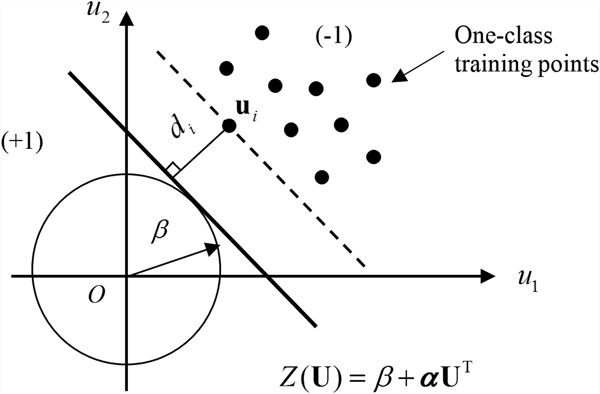
The one-class SVM (Schölkopf et al., Reference Schölkopf, Platt, Shawe-Taylor, Smola and Williamson2001) is a variant of the general SVM and is used for only one class of training points. This method regards the training points available as belonging to the first class and the origin as being the second class. Then the general two-class SVM techniques could be employed. A decision boundary is built by maximizing the distance between training points and the origin, as shown in Figure 1.

Fig. 1. Basic principle of general one-class SVMs.
For m training points ![]() $({\bf x}_1\comma \,y_1)\comma \,{\rm } ({\bf x}_2\comma \,y_2)\comma \,{\rm } \ldots {\comma \,} ({\bf x}_m\comma \,y_m)\comma \,\quad y_i = + 1\comma&InLnBrk; i = 1\comma \,2\comma \, \ldots\comma \, m\comma \,{\rm } {\bf x}\in {\bf R}^n$, belonging to the only one class, the optimization model is given by
$({\bf x}_1\comma \,y_1)\comma \,{\rm } ({\bf x}_2\comma \,y_2)\comma \,{\rm } \ldots {\comma \,} ({\bf x}_m\comma \,y_m)\comma \,\quad y_i = + 1\comma&InLnBrk; i = 1\comma \,2\comma \, \ldots\comma \, m\comma \,{\rm } {\bf x}\in {\bf R}^n$, belonging to the only one class, the optimization model is given by
 $$\left\{ \matrix{\mathop {{\rm min}}\limits_{{\bi \omega} {\comma \,} {\bi \xi} {\comma \,} \rho} \displaystyle{1 \over 2}{\bi \omega} {\bi \omega}^{\rm T} + \displaystyle{1 \over {{\rm mv}}}\sum\limits_{i = 1}^m {\xi_i} -\rho \hfill \cr {\rm s}{\rm. t}{\rm.} \quad{\bi \omega} \cdot \psi \;({\bf x}_i) + \xi_i-\rho \ge {\rm 0\comma \,} \xi_i \ge {\rm 0}\comma \, i = {\rm 1\comma \,2\comma \,} \ldots {\comma \,} m \hfill} \right.$$
in which ω and ρ are the to-be-determined weight vector and bias, respectively. The regularization variable v ∈ (0, 1) indicates the maximum value of the fraction of training data set errors, and ξ = [ξ 1, ξ 2, …, ξ m] is a vector of slack variables that allow point xi to locate on the other side of the optimal hyperplane.
With introducing Lagrange multipliers η i and γ i, the Lagrangian function of Eq. (1) is given by
 $$L({\bi \omega}\comma \, {\bi \xi}\comma \, \rho) + = \displaystyle{1 \over 2}{\bi \omega} {\bi \omega} ^{\rm T} + \displaystyle{1 \over {mv}}\sum\limits_{i = 1}^m {\xi _i} -\rho -\sum\limits_{i = 1}^m {\gamma _i} ({\bi \omega} \cdot \psi \;({\bf x}_i) + \xi _i-\rho )-\sum\limits_{i = 1}^m {\eta _i\xi _i} $$
With the appropriate kernel function K(xi, X) = K(ψ(xi), ψ(X)), the optimization model is then written in the dual form
 $$\left\{ \matrix{\mathop {{\rm min}}\limits_{\bi \gamma} \displaystyle{1 \over 2}\sum\limits_{i\comma \,j = 1}^m {\gamma_i\gamma_jK({\bf x}_i\comma \,{\bf X})} \hfill \cr {\rm s}{\rm. t}{\rm.} \quad{\rm 0} \le \gamma_i \le \displaystyle{1 \over {mv}}{\comma \,} \sum\limits_{i = 1}^m {\gamma_i} = 1 \hfill} \right.$$
Note that when v approaches zero, most of the training points locate inside the estimated support. Then the upper bound of γ i in Eq. (3) tends to infinity, making the second inequality constraint useless, which is similar to the hard margin algorithm used in two-class SVM. Since there is no constraints for bias ρ, the original optimization model can still be solved by assigning a large negative value to ρ (Schölkopf et al., Reference Schölkopf, Platt, Shawe-Taylor, Smola and Williamson2001).
Standard quadratic programing can be used to solve for γ 1, γ 2, …, and γ m. The weight vector of the hyperplane is computed by
And the bias is calculated by
With the determined ω and b, the decision boundary for one-class SVM is given by
A new algorithm for one-class support vector machines with a bias constraint
In this work, we propose a new one-class SVM method with a bias constraint. In the general SVM algorithm, although a bias exists, it is treated separately and does not appear in the optimization model. In the present problem, a bias exists and it is used to formulate a constraint function of the optimization model. The existence of the bias simplifies the optimization model.
The problem arises in the field of system reliability analysis. The proposed method works for the following situation. For the prediction of the reliability associated with a failure mode, repeated reliability testing is performed, and the failure data are recorded until failures occur. Then there is only one class of data. With the failure data, the reliability, which is the probability that the failure mode does not occur, can be estimated. This reliability determines the bias. While more background information about reliability will be provided in the section “Application of the new one-class SVM in system reliability prediction,” the new one-class SVM problem we are dealing with is summarized below.
Information available includes the following:
• A data set of m training points and responses is given by
 $({\bf u}_1\comma \,y_1)\comma \, ({\bf u}_2\comma \,y_2)\comma \, \ldots {\comma \,} ({\bf u}_m\comma \,y_m){\comma \,} \quad {\bf u}\in {\bf R}^n$, y i = −1, i = 1, 2, …, m. Note that different from the general SVM where training points are denoted by
  ${\bf X}$, here we use u for training points because it is a common notation for reliability analysis where the new method will be used. The data set is from reliability testing, and it may include load, dimensional, temperature, and other parameters that cause a failure. The corresponding response is the state of the component under testing, and y i = −1 represents a failure state. All data points belong to the class of failure, and no data points belong to the class of safety.
• We know the shortest distance β from the origin to the domain to which the data set belongs. This distance comes from the known reliability.
The assumptions we make for the new SVM method are as follows:
• We assume that the boundary of the domain to which the data set belongs is a hyperplane. This assumption is valid for reliability applications where the first order reliability method (FORM) (Cruse, Reference Cruse1997) is applicable.
• The hyperplane is given by
(7) $$Y = \beta + {\bi \alpha} {\bf U}^{\rm T}$$
where β is a constant, and α is a unit vector. In the reliability application concerned by this study, β is given and is determined by the reliability estimated from the training points, and α happens to be a unit vector. This assumption does not affect the generality of the proposed method.
Our task is to determine the unit vector α. In sum, our present problem is to find the optimal normal vector α of a hyperplane given its distance to the origin being β and a data set ![]() $({\bf u}_1\comma \,y_1)\comma \, ({\bf u}_2\comma \,y_2)\comma \, \ldots {\comma \,} ({\bf u}_m\comma \,y_m){\comma \,} {\bf u}\in {\bf R}^n$.
$({\bf u}_1\comma \,y_1)\comma \, ({\bf u}_2\comma \,y_2)\comma \, \ldots {\comma \,} ({\bf u}_m\comma \,y_m){\comma \,} {\bf u}\in {\bf R}^n$.
As demonstrated in Figure 2, the problem is to find a hyperplane that is tangent to a hypersphere with a radius of β, and the hyperplane also maximizes the distance from any training points to the hypersphere.

Fig. 2. Basic principle of the proposed one-class SVM.
Denote the distance from ![]() ${\bf u}_i$ to the hypersphere by d i. Points located in the negative region enable Y < 0; otherwise, Y > 0 holds. The minimum distance is given by
${\bf u}_i$ to the hypersphere by d i. Points located in the negative region enable Y < 0; otherwise, Y > 0 holds. The minimum distance is given by
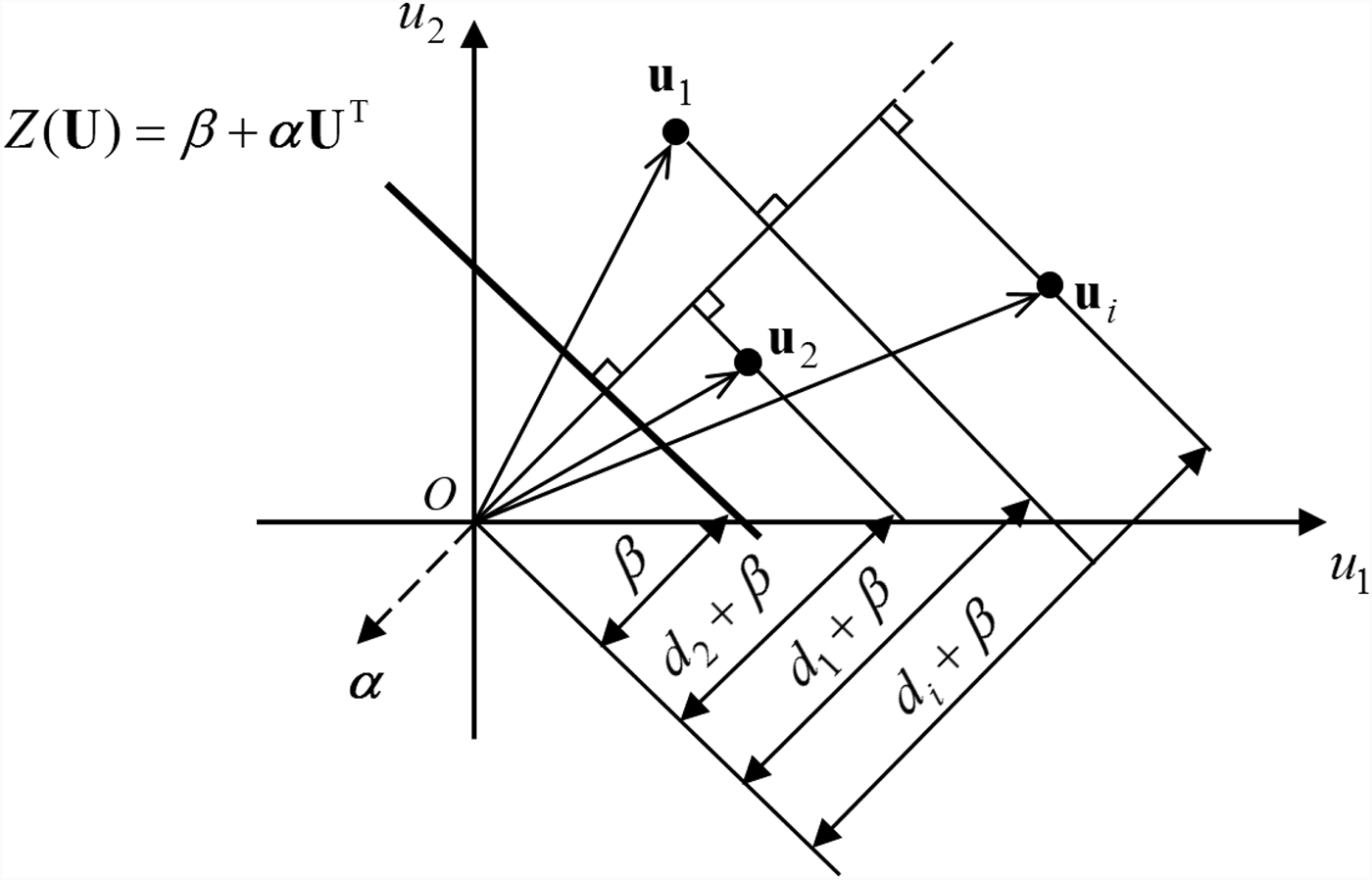
in which the negative sign indicates that the training points locate in the negative side of the hyperplane Z(U), thereby making d positive. Since β is a known constant, d is actually determined by minimizing d i + β , which is equal to ![]() $-{\bi \alpha} {\bf u}_i^{\rm T} $. Note that d i + β indicates the scalar projection of ui onto α. Since
$-{\bi \alpha} {\bf u}_i^{\rm T} $. Note that d i + β indicates the scalar projection of ui onto α. Since ![]() ${\bi \alpha} {\bf u}_i^{\rm T} $ is negative, the direction of α is opposite to that of ui. The geometrical meaning of d i + β is shown in Figure 3.
${\bi \alpha} {\bf u}_i^{\rm T} $ is negative, the direction of α is opposite to that of ui. The geometrical meaning of d i + β is shown in Figure 3.

Fig. 3. Geometric meaning of d i + β.
To construct the optimal hyperplane, our task then becomes to find the maximum d, which can be obtained from the following optimization model
 $$\left\{ \matrix{\mathop {{\rm max}}\limits_{{\bi \alpha}\comma \, d} d \hfill \cr {\rm s}{\rm. t}{\rm.} \quad{\rm -(}\beta + {\bi \alpha} {\bf u}_i^{\rm T}) \ge d\;\;(i={\rm 1\comma \,2\comma \,} \ldots {\comma \,} m{\rm )\comma \,} \hfill} \right.$$
This is the basic model of the proposed one-class SVM with a bias constraint determined by the given constant β. Let h = d + β, and Eq. (9) is rewritten as
 $$\left\{ \matrix{\mathop {{\rm max}}\limits_{{\bi \alpha}\comma \, h} h \hfill \cr {\rm s}{\rm. t}{\rm.} \quad{\rm -}{\bi \alpha} {\bf u}_i^{\rm T} \ge h\;\;(i={\rm 1\comma \,2\comma \,} \ldots {\comma \,} m ){\rm.} \hfill} \right.$$
 Setting ω = α/h, we have ![]() $h = 1/\parallel {\bi \omega} \parallel $. Then Eq. (10) becomes
$h = 1/\parallel {\bi \omega} \parallel $. Then Eq. (10) becomes
 $$\left\{ \matrix{\mathop {{\rm max}}\limits_{\bi \omega} \displaystyle{1 \over {\parallel {\bi \omega} \parallel}} \hfill \cr {\rm s}{\rm. t}{\rm.} \quad{\bi \omega} {\bf u}_i^{\rm T} \le -1(i={\rm 1\comma \,2\comma \,} \ldots {\comma \,} m{\rm )\comma \,} \hfill} \right.$$
which is equivalent to the constrained quadratic programing problem as follows:
 $$\left\{ \matrix{\mathop {{\rm min}}\limits_{\bi \omega} \displaystyle{1 \over 2}{\bi \omega} {\bi \omega}^{\rm T} \hfill \cr {\rm s}{\rm. t}{\rm.} \quad{\bi \omega} {\bf u}_i^{\rm T} + 1 \le 0\;\;(i={\rm 1\comma \,2\comma \,} \ldots {\comma \,} m ){\rm.} \hfill} \right.$$
With Lagrange multipliers λ i ≥ 0, the Lagrangian function is given by
According to the KKT conditions, we have
Substituting Eq. (14) into Eq. (13), the Lagrangian function is rewritten as
 $$\eqalign{ L({\bi \omega}) &= \displaystyle{1 \over 2}\sum\limits_{i\comma \,j = 1}^m {\lambda _i\lambda _j{\bf u}_i{\bf u}_j^{\rm T}} -\sum\limits_{i = 1}^m {\lambda _i\left( {\left( {\sum\limits_{i = 1}^m {\lambda_i{\bf u}_i}} \right){\bf u}_i^{\rm T} -1} \right)} \cr & = \displaystyle{1 \over 2}\sum\limits_{i\comma \,j = 1}^m {\lambda _i\lambda _j{\bf u}_i{\bf u}_j^{\rm T}} -\sum\limits_{i\comma \,j = 1}^m {\lambda _i\lambda _j{\bf u}_i{\bf u}_j^{\rm T}} + \sum\limits_{i = 1}^m {\lambda _i} \cr & = \sum\limits_{i = 1}^m {\lambda _i} -\displaystyle{1 \over 2}\sum\limits_{i\comma \,j = 1}^m {\lambda _i\lambda _j{\bf u}_i{\bf u}_j^{\rm T}}} $$
Thus, the dual form of the quadratic programing problem in Eq. (12) is given by
 $$\left\{ \matrix{\mathop {{\rm max}}\limits_{\bi \lambda} \sum\limits_{i = 1}^m {\lambda_i} -\displaystyle{1 \over 2}\sum\limits_{i\comma \,j = 1}^m {\lambda_i\lambda_j{\bf u}_i{\bf u}_j^{\rm T}} \hfill \cr {\rm s}{\rm. t}{\rm.} \;\;\lambda_i \ge 0{\comma \,} \forall i={\rm 1\comma \,2\comma \,} \ldots {\comma \,} m \hfill} \right.$$
 Solving the optimization model in Eq. (16) yields the Lagrange multipliers λ 1, λ 2, …, λ m. Substituting them into Eq. (14) produces the weight vector ω. The unit vector α is then recovered by ![]() ${\bi \alpha} = {\bi \omega} /\parallel {\bi \omega} \parallel $, which thereby constructs the function Z(U) for the hyperplane. Similar to the general one-class SVM algorithm, the training points satisfying {xi: i ∈ 1, 2, …, m, λi >0} are support vectors by which the optimal hyperplane is finally determined.
${\bi \alpha} = {\bi \omega} /\parallel {\bi \omega} \parallel $, which thereby constructs the function Z(U) for the hyperplane. Similar to the general one-class SVM algorithm, the training points satisfying {xi: i ∈ 1, 2, …, m, λi >0} are support vectors by which the optimal hyperplane is finally determined.
With the known bias β and the acquired normal vector α, the function of the hyperplane is determined by
which is a decision boundary defining the domain of the one class data set and could then be used to predict the state of a new sample. Substitute a new sample uN into Eq. (17). If Y < 0, the new sample belongs to the same class as that of the training points, and y = −1; otherwise, it is outside the domain of the training points and belongs to the class of y = +1.
The proposed one-class SVM algorithm can easily accommodate the bias constraint, which is derived from the given one-class data set. The new algorithm only focuses on this data set without considering the origin as the second class. The optimal hyperplane is constructed based on the hard margin associated with the bias constraint. Specifically, if we regard seeking such an optimal hyperplane as a dynamic process, the general one-class SVM technique attempts to move the hyperplane to the desired position through rotations and translations. While in the proposed method the hyperplane only rotates around the origin while keeping tangent to the hypersphere with a radius of β. In other words, the hyperplane rolls without slipping on the hypersphere. Also, since no slack variables ξ; and regularization parameter v are introduced, the constraints for the optimization model are relatively simple thereby increasing the computation efficiency.
Application of the new one-class SVM in system reliability prediction
System reliability is the probability of a system working normally without failures. Since the system state (safe or failed) is determined by the states of its components and it may be hard to predict the system reliability directly, the system reliability is usually estimated based on component states. Physics-based methods (Cruse, Reference Cruse1997; Mahadevan, Reference Mahadevan and Cruse1997; Hu and Du, Reference Hu and Du2016, Reference Hu and Du2019; Hu et al., Reference Hu, Nannapaneni and Mahadevan2017) and statistics-based methods (Lawless, Reference Lawless1983; Hoyland and Rausand, Reference Hoyland and Rausand2004; Meeker and Escobar, Reference Meeker and Escobar2014; Hu and Du, Reference Hu and Du2017b) are two possible choices for component reliability analysis. We first briefly review the concepts and basic techniques of the two kinds of reliability methods and then explain how the proposed algorithm works for system reliability analysis.
Physics-based reliability methods
Physics-based reliability methods use computational models to estimate reliability, which predict the component failure state based on physical principles. The computational model is called a limited-state function, denoted by ![]() $y = g({\bf X})$, where
$y = g({\bf X})$, where ![]() ${\bf X}$ is a vector of basic random variables, which are root variables that affect the state of the failure mode, such as component shape and dimensions, loadings, material properties, and environmental factors; y is the state variable. For each failure mode, a limit-state function is built. If Y > 0, the state is safe. Otherwise, a failure occurs. The reliability with respect to the failure mode is given by
${\bf X}$ is a vector of basic random variables, which are root variables that affect the state of the failure mode, such as component shape and dimensions, loadings, material properties, and environmental factors; y is the state variable. For each failure mode, a limit-state function is built. If Y > 0, the state is safe. Otherwise, a failure occurs. The reliability with respect to the failure mode is given by
The probability of failure p f is given by
Since it is difficult to compute Eq. (19) analytically, many approximation methods have been proposed, including FORM (Cruse, Reference Cruse1997; Chiralaksanakul and Mahadevan, Reference Chiralaksanakul and Mahadevan2005), the second order reliability method (Zhao and Ono, Reference Zhao and Ono1999), the saddlepoint approximation method (Du and Sudjianto, Reference Du and Sudjianto2004; Hu and Du, Reference Hu and Du2018c), the partial safety factor method (Hu and Du, Reference Hu and Du2018b), and Monte Carlo simulation (MCS) (Green et al., Reference Green, Wang, Alam and Singh2013). In this work, we adopt FORM to approximate a linear form of ![]() $g({\bf X})$, then the component probability of failure could be easily estimated. The procedure of FORM is briefly summarized in the following three steps.
$g({\bf X})$, then the component probability of failure could be easily estimated. The procedure of FORM is briefly summarized in the following three steps.
Step 1: Transform random variables into standard normal variables
Assume that all the random variables in the X-space are independent. The original random variables X = (X 1, X 2, …, X n) are transformed into standard normal random variables U = (U 1, U 2, …, U n) in the U-space. The transformation is given by (Rosenblatt, Reference Rosenblatt1952)
where F i( · ) and Φ( · ) are the cumulative distribution functions (CDF) of X i and a standard normal variable, respectively. The transformation could also be given in the form of
in which T( · ) denotes the transformation function.
Step 2: Approximate a linear limit-state function
After the transformation, the component probability of failure is computed by
FORM then approximates g(T(U)) at the most probable point (Cruse, Reference Cruse1997), and yields a linear limit-state function
Step 3: Compute p f
With the new limit-state function Z(U) in Eq. (23), which is a linear combination of standard normal random variables, p f is calculated by
Statistics-based reliability methods
A statistics-based method relies on field or testing data related to failures of a component. The component reliability R is estimated by
where ![]() $\Pr \{ \cdot \} $ denotes a probability, N f is the number of failed component, and N is the total number of components.
$\Pr \{ \cdot \} $ denotes a probability, N f is the number of failed component, and N is the total number of components.
SVM is widely used with the statistics-based method which creates a reliability model using the provided training data with no need for physical principle of the component. Note that the recorded field or testing data belong to either the safe region or failure region. SVM can therefore identify the safety-failure boundary by solving a binary classification problem (Hu and Du, Reference Hu and Du2017b). As is mentioned above, the general two-class SVM is only available for cases where two classes of training data are provided.
Application of the new method
We now discuss how to use the proposed one-class SVM approach to achieve a linear decision boundary (limit-state function) if only a one-class training data set is given. The details are as follows.
We still use y = g(X) as the component limit-state function, and the original random variables, denoted by X = (X 1, X 2, …, X n) are independent. The counterpart of ![]() ${\bf X}$ in the U-space, denoted by U = (U 1, U 2, …, U n), are standard normal random variables. Given a data set of m training points from reliability testing at failure states as follows:
${\bf X}$ in the U-space, denoted by U = (U 1, U 2, …, U n), are standard normal random variables. Given a data set of m training points from reliability testing at failure states as follows:
The bias β is known, which comes from the component reliability estimated by the supplier using the given training points.
Step 1: Transform ![]() ${\bf X}$ into
${\bf X}$ into ![]() ${\bf U}$
${\bf U}$
Similar to FORM, the transformation is given by
Step 2: Approximate a linear limit-state function based on one-class SVM
According to the proposed one-class SVM discussed in the section “A new algorithm for one-class support vector machines with a bias constraint,” the optimal normal orientation of the to-be-determined decision boundary is given by ![]() ${\bi \omega} = -\sum\nolimits_{i = 1}^m {\lambda _i{\bf u}_i} $, in which λ i is available after solving the dual form of the Lagrangian in Eq. (16), and ui is obtained in step 1. Since the bias β is also available, the linear form of the component limit-state function is then obtained by
${\bi \omega} = -\sum\nolimits_{i = 1}^m {\lambda _i{\bf u}_i} $, in which λ i is available after solving the dual form of the Lagrangian in Eq. (16), and ui is obtained in step 1. Since the bias β is also available, the linear form of the component limit-state function is then obtained by
in which ![]() ${\bi \alpha} = {\bi \omega} /\parallel {\bi \omega} \parallel $.
${\bi \alpha} = {\bi \omega} /\parallel {\bi \omega} \parallel $.
Since β is known, there is no need to recalculate component reliability using Z(U). Z(U) is actually used for the system reliability prediction by integrating with other available limit-state functions from FORM. Next, we will discuss how to do so.
System reliability analysis
System reliability could be estimated either by a physics-based approach, a statistics-based approach, or the integration of both. Predicting system reliability is an important task, especially for systems with outsourced components. Outsourcing is a common practice because more and more industrial firms function like system integrators with numerous components outsourced (Click and Duening, Reference Click and Duening2004), resulting in urgent demand for integrating both statistics- and physics-based approaches. Accurately predicting the system reliability requires complete design information for both in-house and outsourced components, such as the limit-sate functions and distributions of basic random variables. System designers may know everything about the in-house components; however, the design details of outsourced components are usually unavailable since they are proprietary to outside suppliers. This makes it hard to directly use traditional methods for system reliability analysis (Cheng and Du, Reference Cheng and Du2016). To address this issue, the proposed one-class SVM method with a bias constraint is used to reconstruct the limit-state functions for outsourced components, thereby integrating the new algorithm with physic-based methods for accurate system reliability prediction.
A proof-of-concept method (Hu and Du, Reference Hu and Du2017a) has been recently developed, and it validates the feasibility of this study. This work is an extension of the algorithm proposed in Hu and Du (Reference Hu and Du2017a) with a bias constraint derived from the data set provided by the component supplier, such as the reliability data at failure states. We now introduce how to use the proposed method for system reliability prediction. The application scope is summarized as follows:
• The system has m components (failure modes) and m ≥ 2.
• Component states are dependent.
• There are two types of components: (1) type-I components, whose probabilities of failure are obtained through physics-based methods, have available limit-state functions
 $g_i^{\rm I} (\cdot )\comma \, (i = 1\comma \,2\comma \, \ldots {\comma \,} m_1 )$, where m 1 is the component number. (2) For the other m 2(m 2 = m − m 1) type-II components, no limit-sate functions are available, but the data set of training points from fields or testing is provided, and the probabilities of failure are evaluated using a statistics-based method.
• Assume the system is in series.
• Distributions of all basic random variables are known.
For a type-I component, the limit-state functions in the U-space are transformed by
For type-II components, the limit-state functions produced by the proposed one-class SVM is given in the form of
 $$\eqalign{Z_j^{{\rm II}} ({\bf U}) &= \beta _j^{{\rm II}} + \displaystyle{{{\bi \omega} _j} \over {\parallel {\bi \omega} _j\parallel}} {\bf U}^T\cr &= \beta _j^{{\rm II}} + {\bi \alpha} _j^{{\rm II}} {\bf U}^T (\,j= m_1+{\rm 1\comma \,}\;m_1+{\rm 2\comma \,} \ldots {\comma \,} m )$$
 Since the components of U follow a standard normal distribution, the reconstructed limit-state functions ![]() $Z_i^{\rm I} ({\bf U})$ and
$Z_i^{\rm I} ({\bf U})$ and ![]() $Z_j^{{\rm II}} ({\bf U})$ also follow normal distributions
$Z_j^{{\rm II}} ({\bf U})$ also follow normal distributions ![]() $Z_i^{\rm I} ({\bf U}) \sim N(\mu _i^{\rm I}\comma \, \sigma _i^{\rm I} )$ and
$Z_i^{\rm I} ({\bf U}) \sim N(\mu _i^{\rm I}\comma \, \sigma _i^{\rm I} )$ and ![]() $Z_j^{{\rm II}} ({\bf U}) \sim &eqbreak;N(\mu _j^{{\rm II}}\comma \, \sigma _j^{{\rm II}} )$, respectively, in which
$Z_j^{{\rm II}} ({\bf U}) \sim &eqbreak;N(\mu _j^{{\rm II}}\comma \, \sigma _j^{{\rm II}} )$, respectively, in which ![]() $\mu _i^{\rm I} = \beta _i^{\rm I} $ and
$\mu _i^{\rm I} = \beta _i^{\rm I} $ and ![]() $\mu _j^{{\rm II}} = \beta _j^{{\rm II}} $ are their vectors of means, and the covariance of
$\mu _j^{{\rm II}} = \beta _j^{{\rm II}} $ are their vectors of means, and the covariance of ![]() $Z_i^{\rm I} ({\bf U})$ and
$Z_i^{\rm I} ({\bf U})$ and ![]() $Z_j^{{\rm II}} ({\bf U})$ is ρ ij, which will be given in Eq. (32). Thus, the joint PDF of
$Z_j^{{\rm II}} ({\bf U})$ is ρ ij, which will be given in Eq. (32). Thus, the joint PDF of ![]() $Z_i^{\rm I} ({\bf U})$ and
$Z_i^{\rm I} ({\bf U})$ and ![]() $Z_j^{{\rm II}} ({\bf U})$, denoted by ϕ U(u), is actually the PDF of a multivariate normal distribution with a mean vector μ and a covariance matrix Σ. μ is given by
$Z_j^{{\rm II}} ({\bf U})$, denoted by ϕ U(u), is actually the PDF of a multivariate normal distribution with a mean vector μ and a covariance matrix Σ. μ is given by
in which ![]() $\beta _i^{\rm I} (i = 1\comma \,2\comma \, \ldots {\comma \,} m_1 )$ is obtained from FORM, and
$\beta _i^{\rm I} (i = 1\comma \,2\comma \, \ldots {\comma \,} m_1 )$ is obtained from FORM, and ![]() $\beta _j^{{\rm II}} (j = m_1{\rm + 1\comma \,}m_1{\rm + 2\comma \,} \ldots {\comma \,} m )$ is calculated by
$\beta _j^{{\rm II}} (j = m_1{\rm + 1\comma \,}m_1{\rm + 2\comma \,} \ldots {\comma \,} m )$ is calculated by ![]() $ {\beta}_j^{\rm II} = -\Phi ^{-1}(p_{\rm fj} )$. Σ is given by
$ {\beta}_j^{\rm II} = -\Phi ^{-1}(p_{\rm fj} )$. Σ is given by
 $${\bf \Sigma} = \left[ {\matrix{ 1 & {\rho_{12}} & \cdots & {\rho_{1m}} \cr {\rho_{21}} & 1 & {} & {\rho_{2m}} \cr \vdots & \vdots & \ddots & \vdots \cr {\rho_{m1}} & {\rho_{m2}} & \cdots & 1 \cr}} \right]_{m \times m}$$
in which ρ ij is the correlation coefficient between the i-th and j-th components and is computed by
 $$\rho _{ij} = \rho _{\,ji} = \left\{ \matrix{{\bi \alpha}_i^{\rm I} \lpar {{\bi \alpha}_j^{\rm I}} \rpar^{\rm T}\comma \, i \lt j \le m_1 \hfill \cr {\bi \alpha}_i^{\rm I} \lpar {{\bi \alpha}_j^{{\rm II}}} \rpar^{\rm T}{\comma \,} i \le m_1 \lt j \hfill \cr {\bi \alpha}_i^{{\rm II}} \lpar {{\bi \alpha}_j^{{\rm II}}} \rpar^{\rm T}\comma \, m_1 \lt i \lt j \hfill} \right.$$
 From Eq. (29), we find ![]() ${\bi \alpha} _j^{{\rm II}} = ({\bi \omega} _j/\parallel {\bi \omega} _j\parallel) \; (j = m_1{\rm + 1\comma \,}m_1{\rm + &eqbreak;2\comma \,} \ldots {\comma \,} m )$, in which
${\bi \alpha} _j^{{\rm II}} = ({\bi \omega} _j/\parallel {\bi \omega} _j\parallel) \; (j = m_1{\rm + 1\comma \,}m_1{\rm + &eqbreak;2\comma \,} \ldots {\comma \,} m )$, in which ![]() ${\bi \alpha} _j^{{\rm II}} $ has the same direction as ωj.
${\bi \alpha} _j^{{\rm II}} $ has the same direction as ωj.
With μ and Σ available, the complete joint PDF ϕ U(u) is also available and is given by
The probability of system failure is computed by
And the system reliability is
 $$\eqalign{ R_{\rm s} &= \Pr \left( {\bigcap\limits_{i = 1}^{m_1} {-Z_i^{\rm I} ({\bf U}) < 0} \cap \bigcap\limits_{ j = m_1{\rm + }1}^m {-Z_j^{{\rm II}} ({\bf U}) < 0} } \right) \cr & = \int\limits_\Omega {\phi _{\bf U}({\bf u})d{\bf u}} } $$
where Ω is the system safe region defined by
 $$\eqalign{\Omega &= \lcub {{\bf U} \vert -Z_i^{\rm I} ({\bf U}) \lt 0\comma \, -Z_j^{{\rm II}} ({\bf U}) }\cr& \lt 0 (i = {\rm 1\comma \,2\comma \,} \ldots {\comma \,} m_1{\rm ;}j = m_1 + {\rm 1\comma \,}m_1+{\rm 2\comma \, \ldots {\comma \,} m )} \rcub $$
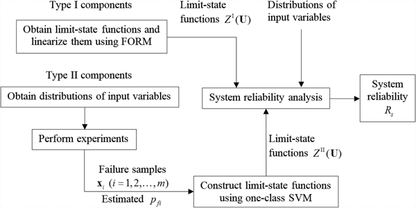
Thus R s can be easily evaluated by solving the integral in Eq. (35), and the probability of system failure is then p f_s = 1 − R s. A schematic diagram of the proposed method is given in Figure 4.

Fig. 4. Schematic diagram of the proposed method.
The proposed method makes the following contributions to reliability analysis: (1) at the component level, it provides a new way to approximate component limit-state functions with only estimated probabilities of failure and limited field or testing failure data. (2) At the system level, since the provided component limit-state functions are linearized using FORM, which produce the same form as the approximated limit-state functions obtained from the proposed one-class SVM, system reliability analysis could be easily conducted. (3) It improves the accuracy of the system reliability prediction because it accounts for the dependency between components automatically. (4) It dramatically reduces the computational cost due to the linear forms of all the limit-state functions.
Examples of methodology validation
Three examples are used to demonstrate the effectiveness and accuracy of the proposed method. Example 1 is a numerical problem showing how to apply the proposed method step by step. Examples 2 and 3 involve engineering problems with multiple failure modes.
Example 1: a numerical problem
A system is comprised of two physical components, and each has one failure mode. If either of components fails, the system fails. There are two independent basic random variables X = (X 1, X 2), where both X 1 and X 2 follow normal distributions of ![]() $X_1 \sim N(12\comma \,1^2)$ and
$X_1 \sim N(12\comma \,1^2)$ and ![]() $X_2 \sim N(40\comma \,2^2)$, respectively. The limit-state function of the first component is available and is given by
$X_2 \sim N(40\comma \,2^2)$, respectively. The limit-state function of the first component is available and is given by
Thus, the component is a type-I component.
FORM produces a linear model, which is given by
in which ![]() $\beta _1^{\rm I} = 3.7225$ and
$\beta _1^{\rm I} = 3.7225$ and ![]() ${\bi \alpha} _1^{\rm I} = (0.6328\comma \,0.7743)$.
${\bi \alpha} _1^{\rm I} = (0.6328\comma \,0.7743)$.
Component two is a type-II component since no model is available. The probability of failure p f2 = 2.5517 × 10⁻⁵ is estimated by a statistics-based reliability method using the recorded testing points, which come from reliability testing.
Although no model is available, to analyze the accuracy, we assume the true model in the X-space is given by
The linear model in the U-space is
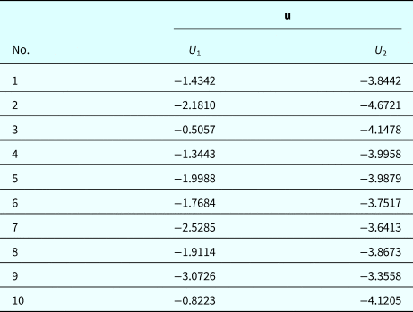
We then use computer experiments to mimic the physical reliability testing. With MCS and the model in Eq. (39), we generate a set of training points and transform them into the U-space as shown in Table 1. We also assume that the value of p f2 given above is known and is equal to the one estimated using Eq. (39).
Table 1. Training points
Assume that the linear model for component two is given by
in which ![]() $\beta _2^{{\rm II}} $ is calculated by
$\beta _2^{{\rm II}} $ is calculated by ![]() $\beta _2^{{\rm II}} = -\Phi ^{-1}(p_{{\rm f}2}) = 4.0508$, and
$\beta _2^{{\rm II}} = -\Phi ^{-1}(p_{{\rm f}2}) = 4.0508$, and ![]() ${\bi \alpha} _2^{{\rm II}} $ is the to-be-determined unit vector. Using the proposed one-class SVM method, we solve for
${\bi \alpha} _2^{{\rm II}} $ is the to-be-determined unit vector. Using the proposed one-class SVM method, we solve for ![]() ${\bi \alpha} _2^{{\rm II}} $ by
${\bi \alpha} _2^{{\rm II}} $ by
 $$\left\{ \matrix{\mathop {{\rm max}}\limits_{\bi \lambda} \sum\limits_{i = 1}^{10} {\lambda_i} -\displaystyle{1 \over 2}\sum\limits_{i\comma \,j = 1}^{10} {\lambda_i\lambda_j{\bf u}_i{\bf u}_j^{\rm T}} \hfill \cr {\rm s}{\rm. t}{\rm.} \quad\lambda_i \ge 0{\comma \,} \forall i={\rm 1\comma \,2\comma \,} \ldots {\comma \,} 10 \hfill} \right.$$
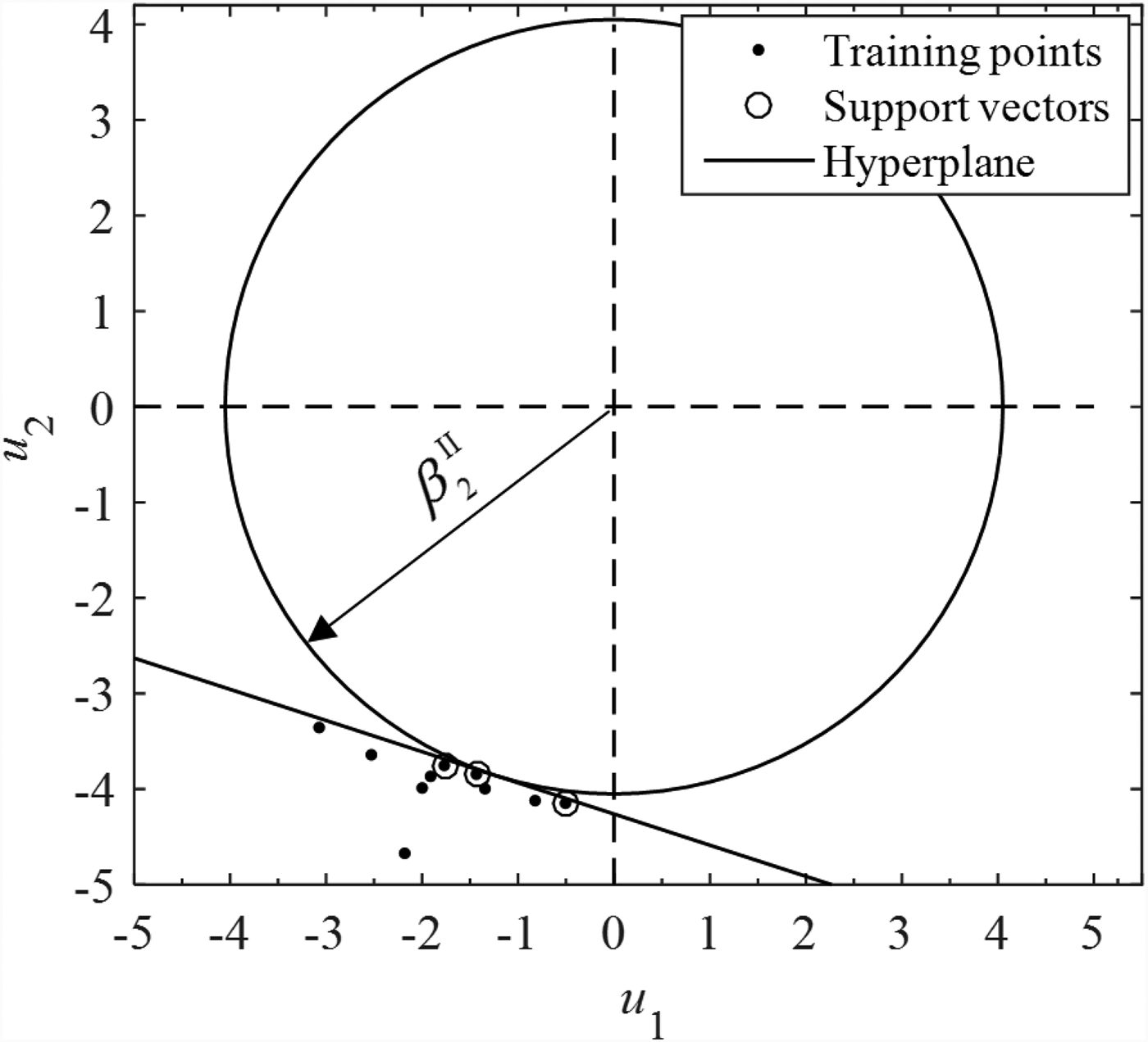
where u1 = ( − 1.4342, − 3.8442), u2 = ( − 2.1810, − 4.6721), …, and u10 = ( − 0.8223, − 4.1205) as shown in Table 1. After solving the above model, we have the Lagrange multipliers λ = (0.0459, 0, 0.0099, 0, 0, 1.734 × 10⁻⁴, 0, 0, 0, 0), and the three support vectors u1, u3, and u6 marked by the circles in Figure 5 are determined by the non-zero multipliers. Substituting λ, u1, u2, …, and u10 into ![]() ${\bi \omega} _2 = -\sum\nolimits_{i = 1}^{10} {\lambda _i{\bf u}_i} $, we obtain the weight vector ω2 = (0.0712, 0.2182), resulting in a unit vector
${\bi \omega} _2 = -\sum\nolimits_{i = 1}^{10} {\lambda _i{\bf u}_i} $, we obtain the weight vector ω2 = (0.0712, 0.2182), resulting in a unit vector ![]() ${\bi \alpha} _2^{{\rm II}} = ({\bi \omega} _2/\parallel {\bi \omega} _2\parallel) =&eqbreak; (0.3101\comma \,0.9507)$. Thus the linear model of component two is reconstructed by
${\bi \alpha} _2^{{\rm II}} = ({\bi \omega} _2/\parallel {\bi \omega} _2\parallel) =&eqbreak; (0.3101\comma \,0.9507)$. Thus the linear model of component two is reconstructed by

Fig. 5. Support vectors and optimal hyperplane.
The corresponding optimal hyperplane is also shown in Figure 5, separating the one class training points (data set at failure state) clearly from the circle with a radius of ![]() $\beta _2^{{\rm II}} $.
$\beta _2^{{\rm II}} $.
The approximated limit-state function in Eq. (43) is very close to the true one given in Eq. (40), thereby leading to high accuracy of system reliability prediction, the details of which are shown below.
Since the components of u follow standard normal distributions, the two dimensional random vector ![]() ${\bf Z} = [Z_1^{\rm I} ({\bf U})\comma \,Z_2^{{\rm II}} ({\bf U})]$ follows a multivariate normal distribution with the joint PDF
${\bf Z} = [Z_1^{\rm I} ({\bf U})\comma \,Z_2^{{\rm II}} ({\bf U})]$ follows a multivariate normal distribution with the joint PDF
where the mean vector μ and covariance matrix Σ are given by
 $${\bf \Sigma} = \left[ {\matrix{ 1 & {\rho_{12}} \cr {\rho_{21}} & 1 \cr}} \right] = \left[ {\matrix{ 1 & {{\bi \alpha}_1^{\rm I} {\lpar {{\bi \alpha}_2^{{\rm II}}} \rpar }^{\rm T}} \cr {{\bi \alpha}_1^{\rm I} {\lpar {{\bi \alpha}_2^{{\rm II}}} \rpar }^{\rm T}} & 1 \cr}} \right] = \left[ {\matrix{ 1 & {0.9324} \cr {0.9324} & 1 \cr}} \right]$$
The system reliability is calculated by
 $$R_{\rm s} = \Pr \lpar {-Z_1^{\rm I} ({\bf U}) \lt 0\cap -Z_2^{{\rm II}} ({\bf U}) \lt 0} \rpar = \int\limits_\Omega {\phi _{\bf U}({\bf u})d{\bf u}} $$
where Ω is the system safe region defined by
Substituting Eq. (44) into Eq. (47), we have p f_s = 1 − R s = 1.0537 × 10⁻⁴.
We now discuss the case where the traditional system reliability method is used and then compare the results from both methods. The traditional method (Yong Cang, Reference Yong Cang1993) assumes that the states of all the components are independent. Then the system reliability is calculated by
where R i is the reliability of the i-th component. The result is given in Table 2 in the “Independence assumption method” column. Although this method is easy to use and effective, it may produce large errors when the components are highly dependent.
Table 2. Results of system reliability from different methods

To verify the accuracy, we also use the true limit-state functions ![]() $g_1^{\rm I} ({\bf X})$ and
$g_1^{\rm I} ({\bf X})$ and ![]() $g_2^{{\rm II (true)}} ({\bf X})$ in Eqs. (45) and (47) to evaluate the system reliability based on FORM and consider this value as a benchmark. The result obtained is 1.0478 × 10⁻⁴. Table 2 shows all the results from different methods. The independence assumption method has a large error of 18.46%, which is due to the neglected strong correlation indicated by ρ 12 = 0.9324. The proposed method produces an error of only 0.56%, which shows much higher accuracy.
$g_2^{{\rm II (true)}} ({\bf X})$ in Eqs. (45) and (47) to evaluate the system reliability based on FORM and consider this value as a benchmark. The result obtained is 1.0478 × 10⁻⁴. Table 2 shows all the results from different methods. The independence assumption method has a large error of 18.46%, which is due to the neglected strong correlation indicated by ρ 12 = 0.9324. The proposed method produces an error of only 0.56%, which shows much higher accuracy.
Example 2: a cantilever beam
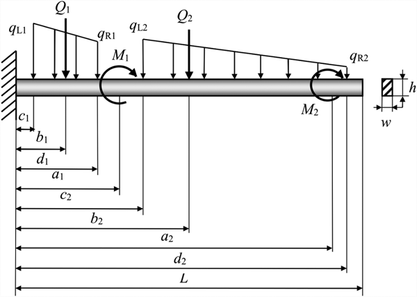
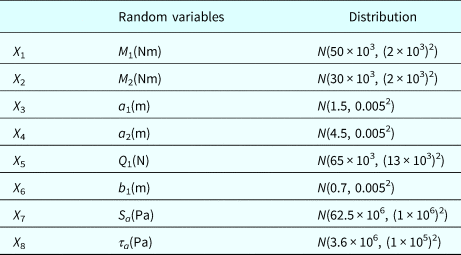
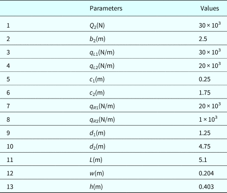
A cantilever beam is subject to moments m 1 and M 2, forces Q 1 and Q 2, and distributed loads denoted by (q L1, q R1) and (q L2, q R2) as shown in Figure 6. Assume that m 1, M 2, and Q 1; the dimensions variables a 1, a 2, and b 1; the yield strength S a; and the allowable shear stress τ a are basic random variables, which are assumed to be independent and listed in Table 3. Deterministic parameters are listed in Table 4.
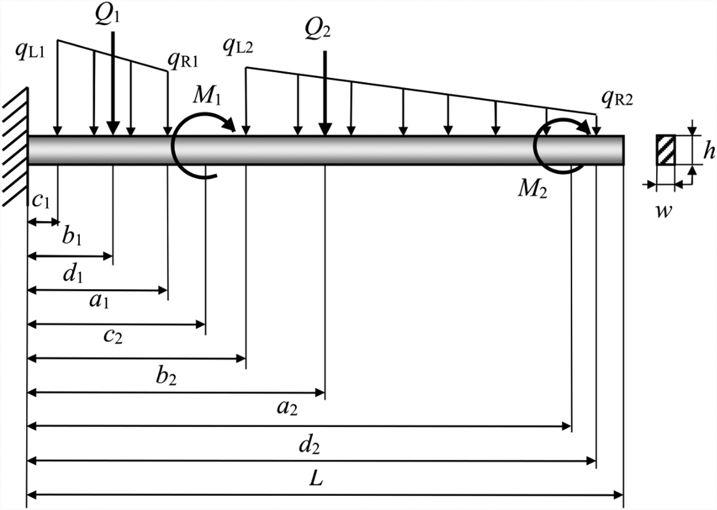
Fig. 6. A cantilever beam system.
Table 3. Basic random variables

Table 4. Deterministic parameters
The cantilever beam fails due to three failure modes, and each is considered as a component, thus the reliability of the beam is regarded as system reliability. The first failure mode is caused by excessive normal stress, and its limit-state function is known and given by
in which M is the bending moment at the root calculated by
 $$\eqalign{ M &= \sum\limits_{i = 1}^2 {M_i} + \sum\limits_{i = 1}^2 {F_ib_i} + \sum\limits_{i = 1}^2 {q_{Li}(d_i-c_i)(d_i + c_i)/2} \cr &\quad + \sum\limits_{i = 1}^2 {[(q_{Ri}-q_{Li})(d_i-c_i)/2][c_i + 2(d_i-c_i)/3]}} $$
Since the limit-state function is provided, this failure mode is treated as a type-I component.
The second failure mode comes from the excessive shear stress with a known limit-state function given by
in which τ a is the allowable shear stress, and τ max is the maximal shear stress computed by
 $$\tau _{\max} = \displaystyle{3 \over {2wh}}\left( {\sum\limits_{i = 1}^2 {F_i} + \sum\limits_{i = 1}^2 {q_{Li}(d_i-c_i)} + \sum\limits_{i = 1}^2 {\displaystyle{{(q_{Ri}-q_{Li})(d_i-c_i)} \over 2}}} \right)$$
Similarly, this failure mode is also a type-I component.
The third failure mode (FM3) is due to the excessive deflection with an unknown limit-state function. It is therefore a type-II component. The probability of failure p f3 due to this failure mode is then evaluated using statistics-based methods with training points. Note that the training points used in this example actually come from computer simulation, since it is hard for us to perform real physical experiments due to lack of measuring devices. Assume the true limit-state function for FM3 is
in which v a = 8.4mm is the allowable deflection, and v max is the maximal tip deflection given by
 $$\eqalign{ v_{\max} &= \displaystyle{1 \over {EI}}\left[ {\displaystyle{{ML^2} \over 2} + \displaystyle{{BL^3} \over 2} + \sum\limits_{i = 1}^2 {\displaystyle{{M_i{(L-a_i)}^2} \over 2}} -\sum\limits_{i = 1}^2 {\displaystyle{{F_i{(L-b_i)}^3} \over 6}}} \right] \cr &\quad + \displaystyle{1 \over {EI}}\left[ {-\sum\limits_{i = 1}^2 {\displaystyle{{q_{Li}{(L-c_i)}^4} \over {24}}} -\sum\limits_{i = 1}^2 {\displaystyle{{(q_{Ri}-q_{Li}){(L-c_i)}^5} \over {120(d_i-c_i)}}}}\right \cr &\quad+ \left{\sum\limits_{i = 1}^2 {\displaystyle{{q_{Ri}{(L-d_i)}^4} \over {24}}}} \right] + \displaystyle{1 \over {EI}}\sum\limits_{i = 1}^2 {\displaystyle{{(q_{Ri}-q_{Li}){(L-d_i)}^5} \over {120(d_i-c_i)}}}}} $$
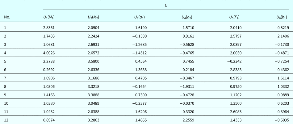
where B is the reaction force at the fixed end. The Young's modulus is E = 200 × 109 Pa, and the moment of inertia is I = wh 3/12. Based on the given limit-state function in Eq. (54), 12 training points at failure states are generated by simulation and are transformed into the U-space as listed in Table 5. Since S a and τ a do not affect the third failure mode, their components U 7 and U 8 are absent in the training points. As discussed previously, p f3 is estimated by a statistics-based reliability method using the data set from reliability testing and is assumed equal to the probability of failure p f3 = 2.864 × 10⁻⁴ produced by FORM with the true-limit state function in Eq. (54).
Table 5. Training points for FM3

Assume the linear model for FM3 is given by
where ![]() $\beta _3^{{\rm II}} = -\Phi ^{-1}(p_{{\rm f}3}) = 3.4442$.
$\beta _3^{{\rm II}} = -\Phi ^{-1}(p_{{\rm f}3}) = 3.4442$. ![]() ${\bi \alpha} _3^{{\rm II}} $ is obtained from the following optimization model
${\bi \alpha} _3^{{\rm II}} $ is obtained from the following optimization model
 $$\left\{ \matrix{\mathop {{\rm max}}\limits_{\bi \lambda} \sum\limits_{i = 1}^{12} {\lambda_i} -\displaystyle{1 \over 2}\sum\limits_{i\comma \,j = 1}^{12} {\lambda_i\lambda_j{\bf u}_i{\bf u}_j^{\rm T}} \hfill \cr {\rm s}{\rm. t}{\rm.} \;\lambda_i \ge 0{\comma \,} \forall i={\rm 1\comma \,2\comma \,} \ldots {\comma \,} 12 \hfill} \right.$$
in which ui represent the training points given in Table 5. Solving the above the model, we obtain the Lagrange multipliers λ = (0, 0, 0.0345, 0, 0.0047, 0.0037, 0.0203, 0, 0, 4.25 × 10⁻⁴, 0, 0.0108); therefore, six support vectors u3, u5, u6, u7, u10, and u12 are determined by the nonzero components λ 3, λ 5, λ 6, λ 7, λ 10, and λ 12 in λ. Then using λ, u1, u2, …, and u12 in ![]() ${\bi \omega} _3 = -\sum\nolimits_{i = 1}^{12} {\lambda _i{\bf u}_i} $, we have ω3 = ( − 0.0787, − 0.2207, 0.0113, − 0.0023, − 0.1157, − 0.0197), which produces the unit vector
${\bi \omega} _3 = -\sum\nolimits_{i = 1}^{12} {\lambda _i{\bf u}_i} $, we have ω3 = ( − 0.0787, − 0.2207, 0.0113, − 0.0023, − 0.1157, − 0.0197), which produces the unit vector ![]() ${\bi \alpha} _3^{\rm II} = ({\bi \omega} _3/\parallel {\bi \omega} _3\parallel) = (-{0.3001\comma \,} - {0.8414\comma \, 0.0430\comma \,} - {0.0087\comma \,} - {\rm 0}{\rm. 4409\comma \,}-{\rm 0}{\rm. 0750})$. Thus, the linear model in Eq. (56) is determined and is given by
${\bi \alpha} _3^{\rm II} = ({\bi \omega} _3/\parallel {\bi \omega} _3\parallel) = (-{0.3001\comma \,} - {0.8414\comma \, 0.0430\comma \,} - {0.0087\comma \,} - {\rm 0}{\rm. 4409\comma \,}-{\rm 0}{\rm. 0750})$. Thus, the linear model in Eq. (56) is determined and is given by
Since the first two failure modes are type-I components, FORM could be directly used with the following linear models:
in which ![]() $\beta _1^{\rm I} = 3.4989$,
$\beta _1^{\rm I} = 3.4989$, ![]() $\beta _2^{\rm I} = 3.2470$,
$\beta _2^{\rm I} = 3.2470$, ![]() ${\bi \alpha} _1^{\rm I} = (-0.181\comma \,-0.181\comma \,0\comma &eqbreak;0\comma -0.826\comma \,-0.046)$, and
${\bi \alpha} _1^{\rm I} = (-0.181\comma \,-0.181\comma \,0\comma &eqbreak;0\comma -0.826\comma \,-0.046)$, and ![]() ${\bi \alpha} _2^{\rm I} = (0\comma \,0\comma \,0\comma \,0\comma \,-0.92\comma \,0)$.
${\bi \alpha} _2^{\rm I} = (0\comma \,0\comma \,0\comma \,0\comma \,-0.92\comma \,0)$.
Thus, vectors ![]() $ [Z_1^{\rm I} ({\bf U})\comma \,\;Z_2^{\rm I} ({\bf U})\comma \,\;Z_3^{{\rm II}} ({\bf U})]$ follow a multivariate normal distribution with the joint PDF given by
$ [Z_1^{\rm I} ({\bf U})\comma \,\;Z_2^{\rm I} ({\bf U})\comma \,\;Z_3^{{\rm II}} ({\bf U})]$ follow a multivariate normal distribution with the joint PDF given by
where the mean μ and covariance matrix Σ are given by
and
 $${\bf \Sigma} = \left[ {\matrix{ 1 & {\rho_{12}} & {\rho_{13}} \cr {\rho_{12}} & 1 & {\rho_{23}} \cr {\rho_{13}} & {\rho_{23}} & 1 \cr}} \right] = \left[ {\matrix{ 1 & {0.7608} & {0.5744} \cr {0.7608} & 1 & {0.4062} \cr {0.5744} & {0.4062} & 1 \cr}} \right]\comma \,$$
where ρ 12, ρ 13, and ρ 23 are the correlation coefficients between ![]() $Z_1^{\rm I} ({\bf U})$ and
$Z_1^{\rm I} ({\bf U})$ and ![]() $Z_2^{\rm I} ({\bf U})$,
$Z_2^{\rm I} ({\bf U})$, ![]() $Z_1^{\rm I} ({\bf U})$, and
$Z_1^{\rm I} ({\bf U})$, and ![]() $Z_3^{{\rm II}} ({\bf U})$, and
$Z_3^{{\rm II}} ({\bf U})$, and ![]() $Z_2^{\rm I} ({\bf U})$ and
$Z_2^{\rm I} ({\bf U})$ and ![]() $Z_3^{{\rm II}} ({\bf U})$, respectively.
$Z_3^{{\rm II}} ({\bf U})$, respectively.
The system reliability is then calculated by
 $$R_{\rm s} = \Pr \lpar {-Z_1^{\rm I} ({\bf U}) \lt 0\cap -Z_2^{\rm I} ({\bf U}) \lt 0\cap -Z_3^{{\rm II}} ({\bf U}) \lt 0} \rpar = \int\limits_\Omega {\phi _{\bf U}({\bf u})d{\bf u}} $$
where Ω is the system safe region defined by
Then Eq. (61) yields p f_s = 1 − R s = 1.022 × 10⁻³.
For validation, we use FORM and all the given limit-state functions ![]() $g_1^{\rm I} ({\bf X})$,
$g_1^{\rm I} ({\bf X})$, ![]() $g_2^{\rm I} ({\bf X})$, and
$g_2^{\rm I} ({\bf X})$, and ![]() $g_3^{{\rm II}} ({\bf X})$ to solve for the true system reliability. Likewise, we also use the independence assumption method. The results are shown in Table 6. The proposed method outperforms the independence assumption method with much higher accuracy.
$g_3^{{\rm II}} ({\bf X})$ to solve for the true system reliability. Likewise, we also use the independence assumption method. The results are shown in Table 6. The proposed method outperforms the independence assumption method with much higher accuracy.
Table 6. Results from different methods

Example 3: a slider mechanism
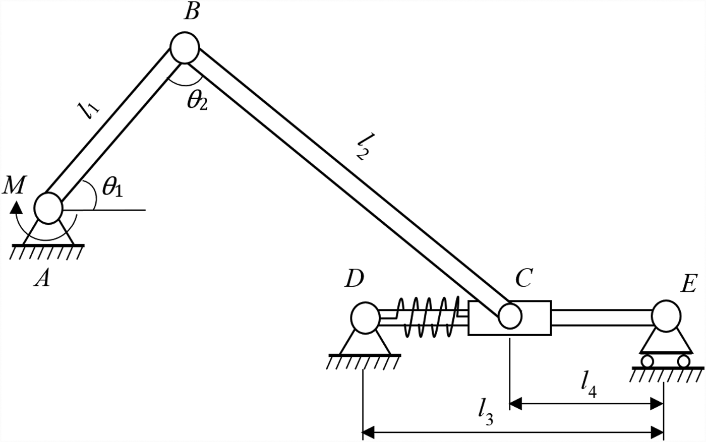
As shown in Figure 7, a slider system consists of four major components. An external moment is applied to joint A. The task is to find the system reliability when θ 2 = π/2.

Fig. 7. A crank-slider system.
Component 1 is beam AB with a length of l 1, and its cross-section is defined by the width b 1 and height h 1. The failure mode (FM1) of AB is the excessive normal stress, and the limit-state function is known and is given by
in which S a1 is the allowable normal stress, and ![]() $S_1 = (M(h_1/2))/(b_1h_1^3 /12)$ is the maximal normal stress developed in the beam.
$S_1 = (M(h_1/2))/(b_1h_1^3 /12)$ is the maximal normal stress developed in the beam.
Component 2 is beam BC with a length of l 2 and a cross-section defined by the width b 2 and height h 2. Beam BC has one failure mode (FM2) due to buckling with a known limit-state function given by
in which P cr = π 2E 2I 2/(Kl 2)2 is the critical force for buckling where ![]() $I_2 = b_2h_2^3 /12$, and F BC = M/l 1 is the internal force in the beam.
$I_2 = b_2h_2^3 /12$, and F BC = M/l 1 is the internal force in the beam.
Component 3 is shaft DE with a diameter of d 4 and a length of l 3. Two failure modes (FM3 and FM4) exist in the shaft which are caused by excessive deflection and excessive normal stress, respectively. The corresponding limit-state functions are known and given by
in which δ a3 is the allowable deflection, and δ 3 is the maximal deflection given by
where E 4 is the Young's modulus of shaft DE. S a4 is the allowable normal stress, and S 4 is the maximal normal stress developed in the shaft and is calculated by
Component 4 is spring CD with one failure mode (FM5) due to excessive shear stress in the spring coils. The limit-state function of FM5 is unknown while the probability of failure is given by p f3 = 1.04 × 10⁻³. Likewise, to simulate the testing, we assume the true limit-state function is given by
in which ![]() $\tau _{a5} \sim N(100 \times 10^6\comma \,(25 \times 10^6)^2){\rm Pa}$ is the allowable shear stress of the spring coil, and τ 5 is the developed maximal shear stress and calculated by
$\tau _{a5} \sim N(100 \times 10^6\comma \,(25 \times 10^6)^2){\rm Pa}$ is the allowable shear stress of the spring coil, and τ 5 is the developed maximal shear stress and calculated by
in which ![]() $D \sim N(34.7 \times 10^{-3}\comma \, 10^{-4}){\rm m}$ is the outer diameter of the spring, and d = 29.5 × 10⁻³m is the spring inner diameter. We then generate 12 training points of X with the corresponding failure states determined by
$D \sim N(34.7 \times 10^{-3}\comma \, 10^{-4}){\rm m}$ is the outer diameter of the spring, and d = 29.5 × 10⁻³m is the spring inner diameter. We then generate 12 training points of X with the corresponding failure states determined by ![]() $g_5^{{\rm II (true)}} ({\bf X}) \lt 0$.
$g_5^{{\rm II (true)}} ({\bf X}) \lt 0$.
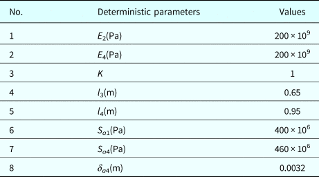
Table 7 shows all the random variables known by the system designers, and Table 8 lists all the known deterministic parameters. Since D and τ a5, denoted by X 9 and X 10, respectively, are only known by the spring supplier, they are not listed in Table 7. There are actually ten basic random variables in the system. For FM5, the training points are provided in the form of (X 1, X 2, X 9, X 10).
Table 7. Random variables
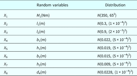
Table 8. Deterministic parameters
At the system level, the five FMs in the system are actually treated as five components. The first four FMs with known limit-state functions ![]() $g_i^{\rm I} ({\bf X}) (i = {1\comma \,2\comma \,3\comma \,4)}$ are type-I components, and FM5 is a type-II component since its limit-state function
$g_i^{\rm I} ({\bf X}) (i = {1\comma \,2\comma \,3\comma \,4)}$ are type-I components, and FM5 is a type-II component since its limit-state function ![]() $g_5^{{\rm II}} ({\bf X})$ is not available.
$g_5^{{\rm II}} ({\bf X})$ is not available.
For type-I components, ![]() $g_i^{\rm I} ({\bf X})$ could be approximated by FORM as
$g_i^{\rm I} ({\bf X})$ could be approximated by FORM as
in which
 $$\eqalign{& \beta _1^{\rm I} = 2.5099\comma \, {\bf \alpha} _1^{\rm I} = (-0.91\comma \,0\comma \,0\comma \,0.16\comma \,0.38\comma \,0\comma \,0\comma \,0\comma \,0\comma \,0) \cr & \beta _2^{\rm I} = 2.6609\comma \, {\bf \alpha} _2^{\rm I} = (-0.60\comma \,1.4 \times 10^{-3}\comma \;\,-0.02\comma \,0\comma \,0\comma \,0.14\comma \,0.79\comma \,0\comma \,0\comma \,0) \cr & \beta _3^{\rm I} = 2.5653\comma \, {\bf \alpha} _3^{\rm I} = (-0.99\comma \,2.6 \times 10^{-4}\comma \;\,1.6 \times 10^{-2}\comma \,0\comma \,0\comma \,0\comma \,0\comma \,0.14\comma \,0\comma \,0) \cr & \beta _4^{\rm I} = 2.4145\comma \, {\bf \alpha} _4^{\rm I} = (-0.99\comma \,2.6 \times 10^{-4}\comma \;\,1.5 \times 10^{-2}\comma \,0\comma \,0\comma \,0\comma \,0\comma \,0.10\comma \,0\comma \,0)} $$
For the type-II component, the limit-state function is reconstructed by the proposed one-class SVM method and is given by
in which ![]() $\beta _5^{{\rm II}} = -\Phi ^{-1}(p_{{\rm f}5}) = 3.0785$ and
$\beta _5^{{\rm II}} = -\Phi ^{-1}(p_{{\rm f}5}) = 3.0785$ and ![]() ${\bi \alpha} _5^{{\rm II}} = (-0.109\comma \,0.066\comma \,0\comma &eqbreak;\,0\comma \,0\comma \,0\comma \,0\comma \,0\comma \,0.068\comma \,0.989)$.
${\bi \alpha} _5^{{\rm II}} = (-0.109\comma \,0.066\comma \,0\comma &eqbreak;\,0\comma \,0\comma \,0\comma \,0\comma \,0\comma \,0.068\comma \,0.989)$.
Then ![]() $Z_i^{\rm I} ({\bf U}) (i = 1\comma \,2\comma \, \ldots {\comma \,} 4 )$ and
$Z_i^{\rm I} ({\bf U}) (i = 1\comma \,2\comma \, \ldots {\comma \,} 4 )$ and ![]() $Z_5^{{\rm II}} ({\bf U})$ follow a multivariate normal distribution with the mean vector
$Z_5^{{\rm II}} ({\bf U})$ follow a multivariate normal distribution with the mean vector ![]() ${\bf \mu} $ and covariance matrix
${\bf \mu} $ and covariance matrix ![]() ${\bf \Sigma} $ given by
${\bf \Sigma} $ given by
 $${\bf \Sigma} = \left[ {\matrix{ 1 & {0.546} & {0.903} & {0.907} & {0.099} \cr {0.546} & 1 & {0.593} & {0.595} & {0.065} \cr {0.903} & {0.593} & 1 & {0.999} & {0.107} \cr {0.907} & {0.595} & {0.999} & 1 & {0.108} \cr {0.099} & {0.065} & {0.107} & {0.108} & 1 \cr}} \right]$$
Thus the probability of system failure is calculate by p f_s = 1-Rs = 0.0133.
Based on the known limit-state functions ![]() $g_i^{\rm I} ({\bf X}) (i = 1\comma \,2\comma \,3\comma \,4)$ and
$g_i^{\rm I} ({\bf X}) (i = 1\comma \,2\comma \,3\comma \,4)$ and ![]() $g_5^{{\rm II (true)}} ({\bf X})$, the true system reliability can be directly obtained by FORM. The results from different methods are shown in Table 9, which demonstrate that the proposed method is close to the true value and outperforms the independence assumption method.
$g_5^{{\rm II (true)}} ({\bf X})$, the true system reliability can be directly obtained by FORM. The results from different methods are shown in Table 9, which demonstrate that the proposed method is close to the true value and outperforms the independence assumption method.
Table 9. Results from different methods

Conclusions
Motivated by the need for creating component models from one-class failure data in system reliability prediction, this study develops a new one-class SVM method for data set that is on the one side of a hyperplane, which is tangent to a hypersphere with a known radius. Different from traditional SVM methods, the new method creates a linear model using both the given data set and the radius; in other words, only the orientation of the hyperplane is determined.
The advantages of the proposed method for system reliability prediction are multifold. At first, it reveals the relationship between component states (safe or failed) with factors that affect the state, such as component dimensions, loading, and environment. Second, the method makes it possible to account for the dependence between component states through the created models. Third, the method obtains a complete probability density function of all the component states. Fourth, the method provides a feasible way to integrate physics- and statistics-based reliability methods. As a result, an accurate system reliability prediction can be produced.
There are several assumptions for the application of the proposed method, such as the distributions of basic random variables are known, the reliability resulting from the FORM is accurate, and no stochastic processes are involved. In our future study, we will extend the method to time-dependent problems where the data set varies with respect to time.
Acknowledgments
This material is based upon work supported by the National Science Foundation under Grant No. CMMI 1562593.
Zhengwei Hu received his PhD from the Department of Mechanical Engineering at the Missouri University of Science and Technology. His research interests include system reliability analysis, statistical modeling, design for reliability, machine learning, and optimization.
Zhangli Hu is currently pursuing his PhD in the Department of Mechanical Engineering at the Missouri University of Science and Technology. His research interests include time-dependent reliability analysis, reliability-based optimization, robust design, and uncertainty quantification.
Dr Xiaoping Du is Professor in the Department of Mechanical and Energy Engineering at Indiana University – Purdue University Indianapolis (IUPUI). Before joining IUPUI, he was Curator's Distinguished Teaching Professor at the Missouri University of Science and Technology. In addition to his academic jobs, he assumed mechanical engineer positions at two companies. He has served as PI for seven grants from the National Science Foundation. He has authored over 100 journal papers. He is Fellow of ASME and currently Associate Editor of Journal of Mechanical Design and Editor of Structural and Multidisciplinary Optimization.


