Design of complex systems

A complex system consists of many components, and the collective behavior of the system can be difficult to model because of the interactions or interdependencies between its parts (Bar-Yam, Reference Bar-Yam and Kiel2002). Much research has been done so far to study ways of designing complex systems. For instance, Arroyo et al. (Reference Arroyo, Huisman and Jensen2018) came up with a bio-inspired, binary-tree-based method for complex system design with fault adaptiveness. The binary-tree branches indicate how organisms achieve adaptive behaviors. Their results show that a strategy-based method can aid designers with innovative analogies, which is useful in providing needed details in design applications (Arroyo et al., Reference Arroyo, Huisman and Jensen2018). Königseder and Shea (Reference Königseder and Shea2016) analyzed various strategies of rule applications in two design synthesis case studies: bicycle frame synthesis and gearbox synthesis, and they found that the effectiveness of each strategy depends on the task scenario. Meluso and Austin-Breneman (Reference Meluso and Austin-Breneman2018) build an agent-based model which simulates the parameter estimation strategy in complex engineering systems on a large scale. They found that accuracy and uncertainty of estimation depend mainly on subsystem behavior but not much on the “gaming” strategy of system engineers’ (Meluso and Austin-Breneman, Reference Meluso and Austin-Breneman2018). McComb et al. (Reference McComb, Cagan and Kotovsky2017) developed a computational model that analyzed how to use the characteristics of configuration design problems into choosing optimal values of teams, such as team size and frequency of interaction. Equations were generated using regression analysis, which was used to predict optimized team values given problem properties (McComb et al., Reference McComb, Cagan and Kotovsky2017). Min et al. (Reference Min, Suh and Hölttä-Otto2016) calculated the structured complexity of complex engineering systems with different levels of decomposition. Their analysis found that the structural complexity of the system is mainly dependent on the lowest level of architectural configurations. Ferguson and Lewis (Reference Ferguson and Lewis2006) developed a method for effective reconfigurable systems design, such as vehicles. Their method focused on identifying changes in system design variables and analyzing the stability of the reconfigurable system with a state-feedback controller. Martin and Ishii (Reference Martin and Ishii1997) proposed a design-for-variety approach, which can help companies quickly adapt their products and address product variation at different generations to reduce the time from products to market. Both qualitative design and quantitative indices have been developed, and the effectiveness of such tools was presented in examples of electronics and automotive industries. Research in previous complex system design requires extensive domain knowledge to build models or draw inspiration from nature, which can be time-consuming and hardly generalizable to different scenarios. Moreover, it still remains a challenging task to generate design rules from global system requirements to local agents’ interactions.

Artificial SOS

Artificial SOS are designed by humans and can have emergent behaviors and adaptability like nature (Reynolds, Reference Reynolds1987). Much research has been conducted in terms of the design of artificial SOS. Werfel (Reference Werfel, Doursat, Sayama and Michel2012) devised a system of homogeneous robots that can build a pre-determined shape with square bricks. Beckers et al. (Reference Beckers, Holland, Deneubourg, Cruse, Dean and Ritter2000) analyzed a robotic gathering task where multiple robots need to patrol a given area in order to collect pucks. As robots have a preference for dropping pucks in high-density areas, the collective positive feedback loop leads to a dense group of available pucks (Ashby, Reference Ashby and Klir1991; Beckers et al., Reference Beckers, Holland, Deneubourg, Cruse, Dean and Ritter2000). Khani and Jin (Reference Khani, Jin and Gero2015) and Khani et al. (Reference Khani, Jin and Gero2016) introduced a social rule-based behavior regulation approach, which can enforce the agents to self-organize and push a rectangle box towards the goal area. Swarms of UAVs can self-organize and accomplish complex tasks, such as shape formation, target detection, and collaborative patrolling, based on a set of cooperation rules (Lamont  et al., Reference Lamont, Slear and Melendez2007; Dasgupta, Reference Dasgupta2008; Ruini and Cangelosi, Reference Ruini and Cangelosi2009; Wei et al., Reference Wei, Madey and Blake2013). Chen and Jin (Reference Chen and Jin2011) adopted an FBR approach, which can assist self-organizing agents in accomplishing complex tasks such as moving towards long-distance targets while avoiding obstacles. Price and Lamont (Reference Price and Lamont2006) tested the effectiveness of the genetic algorithm (GA) in optimizing multi-UAV swarm behaviors. He analyzed the performance of using the GA algorithm in the “destroying retaliating target” task with both homogenous and heterogenous UAVs. The robotic applications mentioned above have demonstrated great potentials for building SOS and the self-organizing system design methods (Chen and Jin, Reference Chen and Jin2011; Khani and Jin, Reference Khani, Jin and Gero2015; Khani et al., Reference Khani, Humann and Jin2016) have had their drawbacks, as discussed in “Introduction”.

Multiagent RL

Multiagent RL applies to multiagent situations. It is based on the basic concept of single-agent RL, such as Q-learning, policy gradient, and actor-critic (Busoniu et al., Reference Busoniu, Babuska and De Schutter2008; Sutton and Barto, Reference Sutton and Barto2018). In comparison to single-agent RL, multiagent learning has a non-stationary learning environment as multiple agents are simultaneously learning.

In order to resolve the issues such as high-dimensionality of state and action spaces in multiagent environments and to approximate state-action values, there has been a move from tabular-based approach to deep RL-based approach in the past several years (Peng et al., Reference Peng, Berseth, Yin and Van De Panne2017; Tampuu et al., Reference Tampuu, Matiisen, Kodelja, Kuzovkin, Korjus, Aru, Aru and Vicente2017; Foerster et al., Reference Foerster, Farquhar, Afouras, Nardelli and Whiteson2018; Rashid et al., Reference Rashid, Samvelyan, Schroeder, Farquhar, Foerster and Whiteson2018). Multiagent systems can be classified into several categories: cooperative, competitive, and mixed cooperative and competitive settings (Tampuu et al., Reference Tampuu, Matiisen, Kodelja, Kuzovkin, Korjus, Aru, Aru and Vicente2017). Cooperative agents share the same rewards, competitive agents (usually in two-agent settings) have opposite rewards, and the mix of cooperative and competitive environments assume agents are not only cooperating but also have individual preferences. In the design of SOS, the focus is on cooperative settings since agents share the same goals.

A natural approach for multiagent RL is to optimize the value functions or the policy of each individual agent. One commonly used value function-based multiagent learning algorithm is independent Q-learning (Tan, Reference Tan1993). In independent Q-learning, each individual's state-action values are trained using Q-learning (Watkins, Reference Watkins1989; Tan, Reference Tan1993), and it is served as a common benchmark in the literature. Tampuu et al. (Reference Tampuu, Matiisen, Kodelja, Kuzovkin, Korjus, Aru, Aru and Vicente2017) expanded previous Q-learning using deep neural networks and applied DQN (Mnih et al., Reference Mnih, Kavukcuoglu, Silver, Rusu, Veness, Bellemare, Graves, Riedmiller, Fidjeland, Ostrovski, Petersen, Beattie, Sadik, Antonoglou, King, Kumaran, Wierstra, Legg and Hassabis2015) to train two independent agents learning how to play the game, Pong. In his simulation, he shows how the cooperative and competitive phenomenon emerges depending on an individual's different reward schemes (Tampuu et al., Reference Tampuu, Matiisen, Kodelja, Kuzovkin, Korjus, Aru, Aru and Vicente2017). Foerster developed a framework called “COMA” and trained multiple agents learning how to cooperate and play StarCraft games (Foerster et al., Reference Foerster, Farquhar, Afouras, Nardelli and Whiteson2018). He utilized a centralized critic network to evaluate decentralized actors and estimated a counterfactual advantage function for each agent and finally allocated credit among them (Foerster et al., Reference Foerster, Farquhar, Afouras, Nardelli and Whiteson2018). In another work by Foerster, he further analyzed the replay stabilization methods he proposed for independent Q-learning in various StarCraft combat scenarios (Foerster et al., Reference Foerster, Nardelli, Farquhar, Afouras, Torr, Kohli and Whiteson2017).

As a multiagent environment is often partially observable, Hauskneche and Stone (Reference Hausknecht and Stone2015) applied deep recurrent networks such as LSTM (Hochreiter and Schmidhuber, Reference Hochreiter and Schmidhuber1997) or GRU (Chung et al., Reference Chung, Gulcehre, Cho and Bengio2014) to facilitate agents’ learning over long time periods. Lowe et al. (Reference Lowe, Wu, Tamar, Harb, Abbeel and Mordatch2017) proposed Multiagent Deep Deterministic Policy Gradient (MADDPG) algorithm, which uses centralized training and decentralized execution. They developed an extension of the actor-critic policy gradient method, which augmented critics with extra information about the policies of other agents and then tested their algorithm in cooperative navigation, predator–pre,y and other environments. Results of their training algorithm show good convergence properties (Lowe et al., Reference Lowe, Wu, Tamar, Harb, Abbeel and Mordatch2017). Drogoul and Zucker (Reference Drogoul and Zucker1998) and Collinot and Drogoul (Reference Collinot and Drogoul1998) introduced a framework for multiagent system design named “Andromeda,” which integrates a machine learning approach with an agent-oriented, role-based approach named “Cassiopeia.” The main idea is to let learning take place within different layers of “Cassiopeia” framework, such as individual roles, relational roles, and organizational roles, which can make the design of multiagent system more systematic and modular (Collinot and Drogoul, Reference Collinot and Drogoul1998; Drogoul and Zucker, Reference Drogoul and Zucker1998). However, as a real multiagent environment can be rather complex, the actions of agents are affected by not only their own roles but also by other agents and the group. Dividing learning into different layers of abstraction may not be feasible. Abramson et al. (Reference Abramson, Ahuja, Barr, Brussee, Carnevale, Cassin, Chhaparia, Clark, Damoc, Dudzik, Georgiev, Guy, Harley, Hill, Hung, Kenton, Landon, Lillicrap, Mathewson, Mokrá, Muldal, Santoro, Savinov, Varma, Wayne, Williams, Wong, Yan and Zhu2020) studied how interactive intelligence can be achieved by artificial agents. They used another learned agent to approximate the role of the human and adopted ideas from inverse RL to reduce the differences between human–human and agent–agent interactive behavior. Results showed that interactive training and auxiliary losses could improve agent behavior beyond what can be achieved by supervised learning (Abramson et al., Reference Abramson, Ahuja, Barr, Brussee, Carnevale, Cassin, Chhaparia, Clark, Damoc, Dudzik, Georgiev, Guy, Harley, Hill, Hung, Kenton, Landon, Lillicrap, Mathewson, Mokrá, Muldal, Santoro, Savinov, Varma, Wayne, Williams, Wong, Yan and Zhu2020).

Most multiagent RL algorithms emphasize achieving optimal cumulative rewards or desirable convergence properties by proposing new training techniques or neural network structures. Many approaches are based on fully observable states, such as the entire game screen. Training of the multiagent reinforcement model is often conducted in prespecified environments with fixed team sizes. Moreover, besides terminal reward often proposed in the literature, it is crucial to identify other important reward functions and test how such reward functions affect the performance of the systems with different task features. For instance, having a rotation reward in multiagent training can play a key role in regulating the system dynamics and facilitating agents’ learning. In addition, the sensitivity of the trained network to different weights of such reward function should be analyzed, which are crucial factors in SOS design. Finally, it is important to develop an evaluation metric of SOS and offer guidelines on how design should be implemented and analyzed in various task situations. Such areas are often ignored in the literature and are the focus of this paper.

Single-agent RL

Multiagent RL is based on single-agent RL, which is used to optimize system performance based on training so that the system can automatically learn to solve complex tasks from the raw sensory input and the reward signal. In single-agent RL, learning is based on the Markov Decision Process defined by a tuple of <S, A, P, R, γ>. S is the state space, composed of the agent's all possible sensing information of the environment. A is the action space, including the agent's all possible actions. P is the transition matrix, which is usually unknown in a model-free learning environment. R is the reward function, and γ is the discount factor for the future rewards. At any given time t, the agent's goal is to maximize its expected future discounted return, $R_t = \sum\nolimits_{t^{\prime}}^T {\gamma ^{{t}^{\prime}-t}r_t}$, where T is the time when the game ends. Also, agents estimate the action-value function Q(s, a) at each time step using Bellman Eq. (1) as an update. E represents the expected value. Eventually, such a value iteration algorithm converges to the optimal value function.

(1)$$Q_{i + 1}( s, \;a) = E[ r + \gamma \mathop {{\rm max}}\limits_{{a}^{\prime}} Q_i( {s}^{\prime}, \;{a}^{\prime}) \vert s, \;a]. $$

In recent years, deep neural networks are introduced as functional approximators to replace the old Q-table for estimating Q-values; such learning methods are called deep Q-learning (Mnih et al., Reference Mnih, Kavukcuoglu, Silver, Rusu, Veness, Bellemare, Graves, Riedmiller, Fidjeland, Ostrovski, Petersen, Beattie, Sadik, Antonoglou, King, Kumaran, Wierstra, Legg and Hassabis2015). A Q-network with weights θ _i can be trained by minimizing the loss function at each iteration i, illustrated in Eq. (2),

(2)$$L_i( {\theta_i} ) = E[ ( y_i-Q( s, \;a; \;\theta _i) ) ^2], $$

where

(3)$$y_i = E[ ( r + {\rm \;}\gamma \mathop {\max }\limits_{{a}^{\prime}} Q( {s}^{\prime}, \;{a}^{\prime}; \;\theta _{i-1}) ] {\rm \;}$$

is the target value for iteration i. The gradient can be calculated with the following equation:

(4)$$\eqalign{\nabla _{\theta _i}L_i( {\theta_i} ) & = {\rm \;}E_{s, a, r, {s}^{\prime}}[\{ r + \gamma \mathop {{\rm max}}\limits_{{a}^{\prime}} Q( {s}^{\prime}, \;{a}^{\prime}; \;\theta _{i-1}) \cr & -{\rm Q}( {\rm s}, \;{\rm a}, \;\theta _i) \} {\rm \;}\nabla _{\theta _i}{\rm Q}( {\rm s}, \;{\rm a}, \;\theta _i) ].}$$

Multiagent RL

There are generally two approaches in multiagent training. One is to train the agents as a team, treating the entire multiagent system as “one agent.” It has good convergence property but can hardly scale up or down. For increasing learning efficiency and maintaining scalability, a multiagent independent deep Q-learning (IQL) approach is adopted. In this approach, A _i, i = 1, …, n (n: number of agents) are the discrete sets of actions available to the agents, yielding the joint action set A = A ₁ × ⋅ ⋅ ⋅  × A _n. All agents share the same state space and the same reward function as the task is cooperative. During training, each agent has its own neural network; they perceive and learn independently except that they share the same reward function and hence the reward value. As the agents are homogeneous and share the same action space, the trained neural networks can be reused and applied in different team sizes. In our multiagent RL mechanism described above, each agent i(i = 1, 2, …, n) engages in learning as if it is in the single-agent RL situation. The only difference is that the next state of the environment, S _t+1, is updated in response to the joint action a _t = {a ₁, a ₂, …, a _n}, instead of its own action a _i, in addition to the current state S _t.

In this research, we first introduced a rotation reward for regulating system dynamics and agents’ behaviors, as shown in Eq. (5), where α ₂ − α ₁ represents the change of angle of the moving object under evaluation, the constant K is between 0 and 1 and is used to discourage the agents’ behaviors that result in rotation of the moving object with more than a certain degree threshold. For example, if K = 0.98, the simulation discourages the rotation of more than 11° as rotation reward R _rot would be negative. This way, the object under control can be rotated constantly to a small degree, which can facilitate the learning of agents by controlling the search space of the agents during exploration with the environment.

(5)$$R_{{\rm rot\;}} = {\rm Cos}( {\alpha_2-\alpha_1} ) -K.$$

After the introduction of the rotation reward, we evaluated the sensitivity of the learning process to the rotation reward – that is, whether good knowledge can be acquired through RL with different weights of rotation reward. Then we looked into the knowledge evaluation issue – that is, how to systematically evaluate SOS performance in different tasks through a set of proposed evaluation metrics: learning stability, quality of knowledge, and scalability. Learning stability measures cumulative reward of agents with increasing training episodes; quality of knowledge is a greedy approach to assess the system performance under the best state-action policy after training; scalability is measured by reusing the trained neural networks to different team sizes, and it tests whether SOS is robust enough to addition or loss of team members.

The box-pushing problem

The box-pushing problem is often categorized as a trajectory planning or piano mover's problem (LaValle, Reference LaValle2006). Many topological and numerical solutions have been developed in the past. In our paper, a self-organizing multiagent deep Q-learning approach is taken to solve the box-pushing problem. During the self-organizing process, each agent acts based on its trained neural network, and collectively all agents can push the box towards a goal without any system-level global control.

In this research, the box-pushing case study was implemented in pygame, a multiagent game package in the Python environment. In the box-pushing case study, each individual agent is trained with its IQL neural network as a member of a team. After the training, the resulting neural networks are applied to the testing situations with various team sizes between 1 and 10. Both training and testing results are analyzed to elicit the learning properties, the quality of learned knowledge, scalability, and robustness of the learned neural networks.

A graphical illustration of the box-pushing case study is shown in Figure 1. The game screen has a width x of 600 pixels and a height y of 480 pixels. Numerous agents (the green squares) with limited pushing and sensing capabilities need to self-organize in order to push and rotate the brown rectangle towards the goal (the white dot with a “+” mark). As there is an obstacle (the red dot) on the path and walls (the white solid lines) along the side, the agents cannot just simply push the box but must rotate the box when necessary (Khani and Jin, Reference Khani, Jin and Gero2015; Khani et al., Reference Khani, Humann and Jin2016). This adds complexity to the task. The box has sensors deployed at its outside boundary. When the outside perimeter of the box reaches the horizontal x-coordinate of the goal, represented as a white vertical line, the simulation is deemed a success.

Fig. 1. A graphical illustration of the box-pushing task.

There are four major tasks of box-pushing, as summarized below. Agents need to move, rotate the box, and keep the box away from potential collisions with walls and obstacles.

• T1 = <Move><Box> to <Goal>

• T2 = <Rotate><Box> to <Goal>

• T3 = <Move><Box> away from <Walls>

• T4 = <Move><Box> away from <Obstacle>

In pygame, the distance is measured by pixels. Each pixel is a single square area in the simulation environment. In this case study, a brown box, which is 90 pixels wide and 225 pixels long, is shown in Figure 1.

In box-pushing, agents have limited sensing and communication capabilities. They can receive information from the sensor on the box, which measures the orientation of the box and senses the obstacles at a range of distances. They have limited storage of observation information: their experiences such as state, action, reward, and next state. They possess a neural network that can transform the perceived state information into action. These assumptions are in line with the definition of the “minimalist” robot (Jones and Mataric, Reference Jones and Mataric2003) and are reasonable with the current applications of physical robot hardware (Groß et al., Reference Groß, Bonani, Mondada and Dorigo2006).

State space and action space

Task state space: Based on the task decomposition and constraint analysis mentioned above, the state space of the box-pushing task is defined as shown in Figure 2. For gathering relevant environment information, a sensor is deployed in the center of the box, which can sense nearby obstacles. The radius of the sensor range is 150 pixels, and the entire circular sensor coverage is split into 8 sectors of equal size, as shown in Figure 2. In this case study, part of the state space captures the state of each sector at any given time: whether the sector is occupied by an obstacle, represented as 1, or not, represented as 0. Furthermore, we assume the sensor can also detect the orientation of the box's x-axis with respect to the location of the goal (Wang and De Silva, Reference Wang and De Silva2006; Rahimi et al., Reference Rahimi, Gibb, Shen and La2018). Denoting the sectors with s₁, s₂, s₃, s₄, s₅, s₆, s₇, s₈, and the box orientation with s ₉, respectively, the state space can be defined as:

(6)$$S = { {s_1, \;s_2, \;s_3, \;s_4, \;s_5, \;s_6, \;s_7, \;s_8, \;s_9} }. $$

Fig. 2. Box-pushing task state representation.

For the example of Figure 2, sectors 3, 5, and 7 are occupied by obstacles. Therefore, the corresponding state attributes s ₃, s ₅, s ₇ are having value 1, and s ₁, s ₂, s ₄, s ₆, s ₈ are 0. In Figure 2, the box angle θ is about 30°. And such degree information can be shaped into the range of [−1,1] by applying s ₉ = (θ − 180)/180 = −0.83. This shaped angle method can facilitate deep Q-network training and is used commonly in practice (Wang and De Silva, Reference Wang and De Silva2006; Rahimi et al., Reference Rahimi, Gibb, Shen and La2018).

Given the above, the state representation of Figure 2 can be expressed as a 9-item tuple <0,0,1,0,1,0,1,0, −0.83>.

During training, each agent is close to the vicinity of the box center, and it can receive the sensor information broadcasted locally among agents. It is assumed that the sensor can also sense the distance from the center of the box to the location of the goal, analogous to real-world radar sensor, and is also like the gradient-based approach in literature where the task field is assumed (Khani and Jin, Reference Khani, Jin and Gero2015; Khani et al., Reference Khani, Humann and Jin2016). Agents can also receive such distance information from the sensor.

Box neighborhood: The box neighborhood is defined as six regions (Khani and Jin, Reference Khani, Jin and Gero2015; Humann et al., Reference Humann, Khani and Jin2016), as shown in Figure 3. During each simulation, an individual agent can move to one of the six regions of the box neighborhood, and that specific neighborhood is the position of the agent. As the individual agent is relatively small, we assume there can be multiple agents in the same region at the same time. This is in line with the definition of the “minimalist” robot (Jones and Mataric, Reference Jones and Mataric2003).

Fig. 3. The six regions of the box neighborhood.

Box dynamics: The box dynamics are based on a simplified physical model. The box movement depends on the simulated force and torque. Forces equal to the sum of vector forces of each pushing agent. Every push carries the same amount of force, which acts from an agent towards the box in the normal direction. The sum of two pushes moves the box 10 pixels in a given direction. Torque is assumed to be exerted on the centroid of the box, and 2 pushes on the diagonal neighborhood of the box (such as positions 2 and 5 each) rotate the box 10°. We assume the box carries a large moment of inertia, and when it hits the obstacle, which is considered rather small, it continues its movement until its expected end position is reached.

Agent action space: The agent action space is defined based on the box neighborhood and simulated box dynamics. At each time step, an agent can choose a place in one of the six regions of the box neighborhoods to push the box. Therefore, the agents share the same action space of A = {a₁, a₂, a₃, a₄, a₅, a₆}, as shown in Figure 3. For instance, if an agent chooses action a₁, it moves to box region “1” and push the box from there, the box moves downwards along the box's y-axis based on the simulated box dynamics, and the same logic applies to other agent actions.

Reward schema and training model

In order to train multiple agents to self-organize and push the box to the final goal area, which is the group level function, we need to design a proper reward schema to facilitate agent training. Adapted from the previous Q-table-based box-pushing reward schema (Wang and De Silva, Reference Wang and De Silva2006; Rahimi et al., Reference Rahimi, Gibb, Shen and La2018), we designed a new reward schema for agents’ box-pushing training. The total reward is composed of four parts: distance, rotation, collision, and goal.

Distance Reward: The reward for pushing the box closer to the goal position is represented as R _dis, and is shown in Eq. (7). The previous distance D _old represents the distance, measured in pixels, between the center of the box and the goal position in the previous time step. D _new represents such distance at the current time step. C _d is a constant, called distance coefficient in our simulation, and is set to 2.5. At each simulation time step, agents calculate the change of distance between the current distance and previous distance based on Eq. (7) and draw its distance reward.

(7)$$R_{{\rm dis}} = ( D_{{\rm old}}-D_{{\rm new}}) \,\ast\, C_d.$$

Rotation Reward: The reward for rotation R _rot is represented in Eq. (8). where α ₁ is the previous time step angle of the box's x-axis with respect to goal position and α ₂, the current angle. The rotation reward is given to discourage the rotation of more than 11°. This way, the box can be rotated constantly with small degrees and avoid large rotation momentum, which can result in a collision with obstacles. The rotation reward is relatively small as it is used only for rotation of the box rather than pushing the box towards the goal, which is the task's goal.

(8)$$R_{{\rm rot}} = {\rm Cos}( {\alpha_2-\alpha_1} ) -0.98.$$

Collision Reward: The collision reward is analogous to the reward schema in common collision avoidance tasks (Liu and Jin, Reference Liu and Jin2018) and is represented in Eq. (9) with R _col. During each simulation step, if there is no collision for the box with either the obstacle or the wall, R _col  = 0. If a collision occurs, a −900 reward is given to all the agents as a penalty.

(9)$$R_{{\rm col}} = \left\{{\matrix{ {-900} \hfill & {\;{\rm if\;collision\;occurs}} \hfill \cr 0 \hfill & {\;{\rm if\;no\;collision\;occurs.}} \hfill \cr } } \right.$$

Goal Reward: The reward for reaching the goal R _goal is represented in Eq. (10). At each simulation step, if the box reaches the goal position, each agent receives a positive 900 reward; if the goal is not reached, the agents do not receive any reward.

(10)$$R_{{\rm goal}} = \left\{{\matrix{ {900\;} \hfill & {{\rm if\;reaching\;goal}} \hfill \cr 0 \hfill & {{\rm if\;not\;reaching\;goal.}} \hfill \cr } } \right.$$

The total reward is a weighted sum of all these rewards, as shown in Eq. (11).

(11)$$R_{{\rm tot}} = w_1\,\ast\, R_{{\rm dis}} + w_2\,\ast\, R_{{\rm rot}} + w_3\,\ast\, R_{{\rm col\;}} + w_4\,\ast\, R_{{\rm goal}}.$$

In our simulations, after repeated testing, the weights were set as w ₁ = 0.6, w ₂ = 0.1, w ₃ = 0.1, w ₄ = 0.2, with the sum of these weights equal to 1, shown in Eq. (12). The weights are chosen so that during each step in training: w ₁ = 0.6, which means agents can have a more immediate reward in terms of whether or not they are closer to the goal; w ₂ = 0.1, which gives a little incentive for agents to rotate the box a small angle; w ₃ = 0.1, to offer some penalty reward if box collides with an obstacle; w ₄ = 0.2, since the agents’ final goal is to reach the target zone, if their goal is achieved, they should be given more rewards than when box collides with an obstacle. The weight for four different rewards is adapted and based on previous research on multiagent box-pushing (Wang and De Silva, Reference Wang and De Silva2006; Rahimi et al., Reference Rahimi, Gibb, Shen and La2018).

(12)$$w_1 + w_2 + w_3 + w_4 = 1.$$

During training, as the agents are homogenous and are cooperating to push the box, they should receive the same rewards. This is the reason why the reward Eqs (7)–(10) are defined based only on the box's position and orientation. In this way, each agent's neural network considers other agents’ actions as part of its environment and learns to explore its action space and also its best policy based on an ε-greedy action selection strategy. Gradually, the agent grasps how to differentiate its actions from other agents to collaboratively push the box towards the goal position, which is the characteristic of multiagent independent deep Q-leaning neural networks.

Experiment design

As aforementioned, the three issues of this research are (1) the stability of the learning dynamics for agents to acquire knowledge for self-organizing behavior regulation, (2) sensitivity of SOS performance to specific reward functions, (3) evaluation of the SOS performance with different task features. To address these issues, we conducted a set of multiagent training and testing experiments, as described below.

Multiagent RL-based agent training

As illustrated in Figure 4, for the multiagent RL-based training process, the Deep Q-learning algorithm described above was applied. The independent variable of the training is the Number of Agents involved in the box-pushing task, denoted by #Tr, varying between 1 and 10. The dependent variables of the training process are the Cumulative Reward signifying the learning behavior of the agents, and a set of #Tr neural networks trained, denoted as, NN _#Tr, representing the learned knowledge.

Fig. 4. Agent training experiment design.

During training, each episode is defined by a complete simulation run, from the starting point to the ending point. The starting point is arranged as shown in Figure 1, where the agent positions are randomly assigned while the box's initial position and the goal position are both fixed. For the ending point, there are three different situations: (1) the box is pushed into the target position, (2) the box collides with the obstacle or any sidewall, and (3) the simulation reaches the maximum number of 500 training steps (each time an agent chooses its action, it is considered one training step). When any one of the three situations happens, a simulation run is completed, and the episode finishes.

One training process in the experiment goes through 16,000 episodes. The numbers are chosen because they are the thresholds for achieving training stabilization at the minimum training cost. In order to maintain statistical stability, each training was run 100 times with different random seeds. The mean value of the 100 cumulative rewards of a corresponding episode is used as the reward value of that episode and plotted as the solid colored lines in the cumulative reward plots in the subsequent part of “Case study box-pushing”. At the same time, the standard errors are plotted as green spreads around the mean values.

As shown in Figure 4, the two dependent variables of the training process are cumulative rewards and the resulting neural networks, representing the team learning behavior and the agents’ learned knowledge, respectively. Details of these variables are discussed subsequent part of “Case study box-pushing”.

Table 1 summarizes the training parameters used in the simulations. Replay memory size is 1000, and 32 mini-batches are randomly sampled from the replay memory during each training step. The discount factor is 0.99, and the learning rate is 0.001. Total training episodes are 16,000. The ε-greedy action selection algorithm was followed where ε is annealed from 1.0 to 0.005 over 100,000 training steps during training. Agents choose actions from entirely random (i.e., ε = 1.0) to nearly greedy (ε = 0.005). The target neural networks are updated at every 200 training steps to stabilize the training. Training the network of each agent consists of an input layer of 9 states, a hidden layer of 16 neurons, a dueling layer (Wang et al., Reference Wang, Schaul, Hessel, Hasselt, Lanctot and Freitas2016), and output 6 state-action values.

Table 1. Simulation parameters

Testing and performance evaluation

The neural networks that are acquired from the MARL-based training are evaluated through testing simulations. Figure 5 illustrates the design of the testing experiment, in which #Tr indicates the number of agents trained and #Ts is the number of agents being tested.

Fig. 5. Testing experiment design and performance evaluation.

There are three independent variables in the testing experiment. They are: learned neural networks NN _#Tr, agent team size (1, …, 10), and noise level (10%). The noise level is defined by the percentage in which the agents choose random actions instead of greedy ones during testing runs. This variable is introduced to model system malfunctions, such as sensor errors and agent disabilities. By correlating the system response to the noise levels, the robustness of the trained neural networks can be evaluated.

When the number of trained agents #Tr is not the same as the number of testing agents #Ts (i.e., #Tr ≠ #Ts), there exists a mismatch for deploying the neural networks. To resolve this mismatch, for cases of #Tr < #Ts, one or more randomly selected networks are repeatedly deployed in the test case. When #Tr > #Ts, then #Ts networks are randomly selected for the testing team agents.

There is one dependent variable performance score in the testing experiment design, as shown in Figure 5, which indicates the quality of the learned knowledge and scalability as it is trained (#Tr = #Ts) and when it is applied in knowledge transfer testing situations (#Tr  ≠#Ts), respectively. Furthermore, correlating the performance score with the noise level helps assess the robustness to noise.

As mentioned above, for each training situation, that is, given #Tr, there are 100 training runs. At the end of each training run, a greedy testing simulation is carried out to evaluate whether the box-pushing is successful. The training performance score, in this case, is defined by the percentage of the number of successful runs. Usually, the training performance score is greater than 60%, except for the team of one agent, which is close to 30%, as will be discussed below.

From the more than 60 successful runs of each training situation (#Tr), 50 sets of neural networks are randomly selected for testing cases. Again, for statistical stability, each selected set of neural networks is simulated 100 times, and the performance score is the percentage of the successful ones among the 100 simulations. This way, after 50 × 100 testing runs, the average performance score of the 50 sets of neural networks is used as the performance score of the testing situation (#Tr, NoiseLevel).

Self-assembly problem

A graphical illustration of a self-assembly case study is shown in Figure 10. The game screen has 800 × 800 pixels. Numerous agents (the green squares) with limited pushing and sensing capabilities need to self-organize in order to push and rotate the box (the brown rectangle) towards the static target box (the gray rectangle box) and form a T-shape structure centered at the target. The agents cannot just simply push the box but have to rotate the box when necessary (Khani and Jin, Reference Khani, Jin and Gero2015; Khani et al., Reference Khani, Humann and Jin2016). This adds complexity to the task. Pymunk, a physics simulation module, was used to build the case study model. In pymunk, the distance is measured by pixels. As an example, the brown box is 60 × 150 pixels, and the gray box is 60 × 210 pixels.

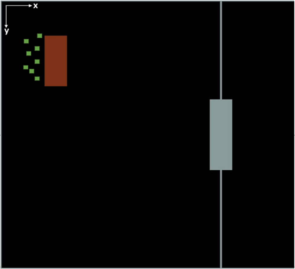
Fig. 10. Graphical illustration of self-assembly task.

State space and action space

The state space of the self-assembly task is defined as S =   < s, α, β, ω, v >, as shown in Figure 11a and Table 2.

Fig. 11. Box state and neighborhood: (a) box state representation, (b) six regions of box neighborhood.

Table 2. State space definition

For gathering the state information, a sensor is deployed in the center of the moving box, which can sense nearby obstacles or targets with a radius of 200 pixels, and the entire circular sensor coverage is equally split into 24 sectors. The vicinity situation is modeled by s = {s ₁, s ₂…, s ₂₄} with s _i representing the corresponding sector situation: has nothing or obstacle or target. In the state of Figure 11a, three obstacles are detected.

The box neighborhood is defined as six regions (Humann et al., Reference Humann, Khani and Jin2014; Khani and Jin, Reference Khani, Jin and Gero2015), as shown in Figure 11b. The box dynamics are based on the pymunk physics model. The mass of the box is 1 kg. An agent can push the box from its position. Every push carries the same amount of impulse acting on the center of one of the box regions from an agent towards the box. The magnitude of an impulse is 1(N ⋅ s), and the box will have a change of velocity of 1 m/s in the pushing direction and a change of angular velocity of around 1°/s if agents push on one of the longer sides of the box neighborhood. For every step in the simulation, agents perform an action and wait for 1 s until the next push is carried out. The agent action space is the same as the box-pushing case study, as shown in Figure 11b.

Reward schema

The reward schema follows the same format as the previous case study, and the total reward is composed of four parts: distance, rotation, collision, and goal.

Distance Reward: The reward for pushing the box closer to the goal position is represented as R _dis, and is shown in Eq. (14). Distance coefficient C _d is set to 0.02.

(14)$$\;R_{{\rm dis}} = {\rm \;}( D_{{\rm old}}-D_{{\rm new}}) \,\ast\,C_d.$$

Rotation Reward: The reward for rotation R _rot is represented in Eq. (15), where α ₁ is the previous time step angle between the center of the target box with respect to the moving box's x-axis, and α ₂ is the current angle. C _r is called rotation coefficient and is set to 0.1.

(15)$$R_{{\rm rot}} = ( {{\rm Cos}( {\alpha_2-\alpha_1} ) -0.98} ) \,\ast\, C_r.$$

Collision Reward: The collision reward is represented in Eq. (16) as R _col,

(16)$$R_{{\rm col}} = \left\{{\matrix{ {-10\;} \hfill & {{\rm if\;collision\;occurs}} \hfill \cr 0 \hfill & {{\rm if\;no\;collision\;occurs}}. \hfill \cr } } \right.$$

During each simulation step, if there is no collision for the box with the wall, R _col = 0. If a collision occurs, a −10 reward is given to all the agents as a penalty.

Goal Reward: The reward for reaching the goal R _goal is represented in Eq. (17),

(17)$$R_{{\rm goal}} = {\rm \;}\left\{{\matrix{ {100\,\ast\,\vert {{\rm Sin}( \alpha ) } \vert \,\ast\,\vert {{\rm Cos}( \beta ) } \vert } \hfill & {{\rm if\;reached\;goal}} \hfill \cr 0 \hfill & {{\rm if\;no\;reaching\;goal}}. \hfill \cr } } \right.$$

α and β are shown in Table 2. During simulation, if the box reaches the target box and form a perfect T-shape, each agent receives a 100 reward; if reached the target box but slightly off angle, the reward is between 0 and 100; if the target is not reached, the agents do not receive any reward. The total reward is the sum of all the rewards, as shown in Eq. (18). The simulation parameters of our algorithm can be seen in Table 3.

(18)$$R_{{\rm tot}} = R_{{\rm dis}} + R_{{\rm rot}} + {\rm \;}R_{{\rm col}} + {\rm \;}R_{{\rm goal}}.$$

Table 3. Training simulation parameters and values

Issue and experiment setup

The case study is focused on three issues: (1) achieving stable learning dynamics by investigating the impact of rotation reward, (2) sensitivity of SOS to different weights of rotation reward function, (3) evaluation of the SOS performance by analyzing the quality of learned knowledge and assessing the robustness of the learned neural network knowledge in the context of varying team sizes and environmental noise.

The number of agents i during training was varied between 4 and 40, with 4 agents in between, that is, 4 ≤ i ≤ 40. The training yields i different neural networks denoted as N _i which is a set of i networks. To evaluate the robustness of the acquired network knowledge, each N _i was applied to the testing cases with j number of agents, and j was varied between 4 and 40, with 4 agents in between, that is, 4 ≤ j ≤ 40. The notation $N_i^j \;( {4 \le i \le 40; \;4 \le j \le 40} ) \;$describes the situation where the network knowledge obtained from the training of i agents is applied to the testing case of j agents. It is conceivable that there are 10 training cases but 100 testing cases. When the testing case agent number j is larger than the training agent number i, that is, i < j, four or more randomly selected networks are repeatedly deployed in the test case. When i > j, then j networks are randomly selected from N _i for testing simulations.

For maintaining statistic stability, for each i agents team, the agents are trained 100 times with different random seeds, resulting in neural networks N _il, 4 ≤ i ≤ 40; l = 1, 2, …, 100. To evaluate the performance of a specific N _il after training, the goal reward of Eq. (17) is used as the performance score. The maximum score is 100, which is when the perfect T-shape is formed in the middle of the target box. For a given i, all 100 networks N _il were collected as the network dataset from which a specific N _il is randomly selected to test j-agent teams, $N_{il}^j$. The testing simulation for a given j-agent team is also run 100 times, and the mean cumulative reward values and performance scores are used in the plots shown in Figures 13–16.

Quality of learned knowledge

The quality of the learned knowledge is evaluated by a performance score. For each i agents team, the agents are trained 100 times with different random seeds, resulting in neural networks N _il, 4 ≤ i ≤ 40; l = 1, 2, …, 100. The performance score of each N _il is evaluated using the goal reward of Eq. (17). The standard error of the mean is also calculated for each team size based on the 100 different performance scores of each random seed. Figure 14 illustrates the results of the performance score of the trained teams of different sizes. Similar to the box-pushing case study, the quality of the learned knowledge depends on the team size: higher-quality knowledge can be acquired for the team sizes at the “magic” number 20 or 24 compared to smaller and larger teams. Finding the “magic” number – that is, the matching point between the task complexity and team complexity – is crucial in acquiring high-quality knowledge through multiagent RL.

Fig. 14. Performance score with a different number of agents in self-assembly task.

We also tested the sensitivity of quality of knowledge with respect to different weights of rotation reward in various team sizes: 1, 2, 4, 12, and 24. During training, the rotation reward is multiplied by a weight factor W _f in addition to its original weight 1, as shown in Eq. (19). A list of values was chosen for W _f: 0, 0.1, 1, 10, 100. After training, with the new trained neural networks N _il, we evaluated the quality of learned knowledge using the same evaluation method: performance score.

(19)$$R_{{\rm tot}} = R_{{\rm dis}} + R_{{\rm rot}}\,\ast\, w_f + R_{{\rm col\;}} + R_{{\rm goal}}.$$

The results of the sensitivity analysis are shown in Figure 15. The error bar shows the standard error of the mean of the performance score with trained neural networks N _il. When agents of various team sizes are trained with W _f = 100, agents ultimately learned how to rotate the box for an extensive period of time in order to accumulate rotation reward instead of learning how to form the T-shape structure. The performance score is indicated with a black rectangle, which represents the inferior quality of knowledge learned when W _f is very big. Except W _f = 100, when the number of agents is 1, there is not a big difference between the quality of knowledge trained with various weight factors of rotation reward. This is because one agent can only move the box with a change of angular velocity of around 1°/s, which is not a very large angle. Thus, having a rotation reward as a penalty reward is not very useful in this case. However, when agent sizes reach 2, 4, and beyond, the quality of knowledge learned is largely dependent on the weights of rotation reward. When W _f = 0 and W _f = 0.1, the effect of regulating agents’ behavior is not very strong, and the performance score is low. When W _f = 1 and W _f = 10, there is enough regulation, and agents can reach the full potential of learning, and the final performance score is most optimal. Thus, for the self-assembly task, it is always advised to introduce some rotation reward, and the weight of such rotation reward cannot be too small nor too big, especially when the agent team size is relatively large: greater than one.

Fig. 15. Sensitivity analysis of performance score with a different number of agents with a different weight factor of rotation reward in self-assembly task.

Scalability and robustness

The scalability of the learned neural network knowledge to different team sizes and the robustness to various noises are two important issues for this case study. Applying neural network trained with i-agent teams to test and assess the performance of j-agent teams, that is, $N_i^j \;( {4 \le i \le 40; \;4 \le j \le 40} )$, allows us to assess the scalability. Further, introducing 10% random agent actions helps evaluate the robustness of the trained networks. The results are shown in Figure 16. The curves with different colors in the figure represent the training of i-agent teams. For example, Tr4 means training of the 4-agent team and Tr8 8-agent team. The horizontal axis indicates j-agent testing teams. The vertical axis shows the performance score of testing [Eq. (17)], with error bars showing the standard error of the mean.

Fig. 16. Transfer performance score with a different number of transfer agents with error bars indicating the standard error.

Similar findings can be drawn compared to the box-pushing case study. As shown in Figure 16, when the trained networks are applied to the same team size, $N_i^i$, agents have a performance score of above 90. As the team size i increases, the performance score of testing runs $N_i^i$ first increases and then decreases, indicating that there is a threshold of the effect of adding more agents. In this case study, the threshold is around 20.

Like the box-pushing case study, transferring learned knowledge downward is less effective compared to doing so upward in terms of team size. This is because during scaling upward, the extra agents can be considered as extra noise, and the system is robust to the impact of “noise.” Scaling downward is more detrimental as the system loses some knowledge within its learned neural networks.

Implications for future SOS design

Although it is worth mentioning that the findings and insights described above are limited to the two case studies reported in this paper, some general guidelines for future SOS design can be derived as follows.

Adding more agents to the system increases system complexity. The “magic” team size is the point where system complexity matches task complexity and has optimal learning stability, quality of knowledge, and scalability. Magic team size is dependent on the type of tasks and system dynamics and is insensitive to the weights of rotation reward during training. Designers can test hypothetical “magic” team sizes using multiagent RL to obtain maximum system performance. For example, from the training stability perspective, at “magic” team size, training becomes most stable and reaches the maximum cumulative reward. From an evaluation perspective, magic team sizes should have a better quality of the learned knowledge and are most robust in response to environmental noises among all team sizes tested.

Learning stability, quality of knowledge, and scalability are three metrics that can be used to assess the SOS. Depending on the type of task, the results of each evaluation measurement can vary.

Learning stability: For tasks with fixed terminal rewards, for example, box-pushing, when agents successfully push the box to the goal, they can get a fixed terminal reward. Failure to push the box to the goal area leaves agents with zero terminal rewards. The variation between the learning stability of agents of various sizes can be manifested with cumulative reward plots as there is a big difference of reward between successful pushing and unsuccessful pushing. For the self-assembly task, the goal reward is based on the final orientation of the box; it is a variational reward depending on the terminal position and is in the range of 0–100. Thus, in self-assembly tasks, it is hard to differentiate between the learning stability of a different number of agents using cumulative reward plots.

Quality of knowledge: Unlike learning stability, which evaluates the learning behavior of agents during training, quality of knowledge assesses the learned knowledge of agents after training. The performance score is a numerical value that measures the quality of knowledge learned. In both box-pushing and self-assembly case studies, quality of knowledge measurement is an effective tool in assessing the learned knowledge of SOS because it can represent slight differences in values by using a performance score, which can be used to determine the “magic” team size of the SOS. In the box-pushing case study, for specific team size, the quality of knowledge is insensitive to the weight of rotation reward. This is because the final goal is not strictly related to the box orientation, and the presence of an obstacle along the pushing trajectory regulates agent behaviors and reduces the need for rotation reward in regulating agents’ actions. However, in the self-assembly task, the inclusion of rotation reward is essential in obtaining the best quality of knowledge. This is because the self-assembly task does not have obstacles along the box's trajectory, and the final position and orientation of the box are critical in accomplishing the task.

Scalability: Scalability is another measurement that is used after training. In both case studies, scaling upward to a higher team size has less impact on system performance during the transfer of knowledge than scaling downward. This is because a neural network is more robust to the noise generated by extra agents than losing knowledge within its team.

Future SOS design should consider the features of the tasks, such as the ultimate goal of the task and whether there are physical constraints like obstacles presented, and introduce appropriate behavior regulation reward, for example, rotation reward during training. Finally, designers can selectively choose three metrics mentioned in our paper to evaluate their system performance depending on the type of task.