1. INTRODUCTION
Layout describes the arrangement of different elements within a given area for a particular purpose. Layout problems can be found in various fields, from the design of timetables or circuit boards to the arrangement of abstract elements in a graph, the organization of the boxes of a shipload or the placement of metal parts to be cut out, and not least the arrangement of rooms in a floor plan or of buildings in an urban neighborhood (Hower & Graf, Reference Hower and Graf1996). For solving layout problems, certain criteria usually have to be taken into account. The elements, for example, should not overlap, and their organization should be as compact and efficient as possible. In this paper, we focus on two-dimensional layouts because this is usually sufficient in the field of architecture, but there is also computational support for solving three-dimensional layout problems (Cagan et al., Reference Cagan, Shimada and Yin2002).
Various floor planning systems have been developed to address and solve the above-mentioned problems, some of which we describe in Section 2. Because it is difficult to compare the advantages and disadvantages of different generative mechanisms with each other, we propose some useful criteria for evaluating the algorithms used and apply them to compare two layout solvers. We have chosen dense packing and subdivision algorithms as the two layout solvers we compare in this paper, because they are well suited for user interaction (Harada et al., Reference Harada, Witkin and Baraff1995). Both algorithms are discussed in detail in Section 3. In the scenarios we discuss here, we start from a fixed building outline and address the two-dimensional arrangement of individual rooms. The dimensions of the rooms are flexible within given minimum and maximum bounds, but rooms have to adhere to a predefined surface area. The sum of the areas of the rooms to be arranged corresponds to the total area defined by the building outline. In addition, specific neighborhood relationships between the rooms have to be ensured. Both methods are analyzed and compared using two different layout scenarios, which are discussed and presented in Section 4. Section 5 presents and discusses the analyses, which include the speed with which solutions are generated, the reliability with which optimal solutions can be found, and the number of different solutions that can be found overall. To conclude, we give a brief outlook of possible further developments in Section 6.
2. RELATED WORK
Solving layout problems using computer-based methods is a key issue for the application of artificial intelligence in the field of architecture. Layout problems are usually very complex problems that have to meet a variety of requirements. With each factor that needs to be considered in a layout design (e.g., number of rooms), the number of possible solutions increases exponentially (March & Steadman, Reference March and Steadman1974). From the perspective of complexity theory, layout problems fall into the category of so-called NP-complete problems.
Since the early 1960s, various methods have been developed for the computer-based solution of layout problems (Whitehead & Eldars, Reference Whitehead and Eldars1964; Frew, Reference Frew1980). All of these methods have in common that they employ a generative mechanism for the creation of alternative variations and an evaluation mechanism to assess these variations (Mitchell, Reference Mitchell1998). A range of solutions has been developed for the appropriate arrangement of rectangular spaces for both general (Krishnamurti & Earl, Reference Krishnamurti and Earl1998) and architectural applications (Mitchell et al., Reference Mitchell, Steadman and Liggett1976). Previous reviews of the development of various approaches to solving this problem (Homayouni, Reference Homayouni2000, Reference Homayouni2006) have proposed some possible classifications. Kalay (Reference Kalay2004) describes three primary method categories that are relevant to layout systems: procedural, heuristic, and evolutionary methods. For our investigation, we will use evolutionary algorithms (EAs). Algorithms for the exhaustive generation of building floor plans were already being developed in the 1980s (Galle, Reference Galle1981). In the 1990s, a system for generating layouts using constraint programming was developed under the name SEED (Flemming & Woodbury, Reference Flemming and Woodbury1995), which is based on the ABLOOS Framework (Coyne & Flemming, Reference Coyne, Flemming and Gero1990). ABLOOS is in turn a hierarchical extension of a system named LOOS (Flemming, Reference Flemming1989), which uses orthogonal structures for the representation of loosely packed arrangements of rectangles. Early examples of the use of evolutionary approaches for layout planning in architecture include those by Gero and colleagues (Gero & Kazakov, Reference Gero and Kazakov1996; Schnier & Gero, Reference Schnier, Gero and Gero1996; Jo & Gero, Reference Jo and Gero1998; Rosenman & Gero, Reference Rosenman, Gero and Bentley1999).
The study we present in the scope of this paper focuses on two known generative methods for dense packing: first, a heuristic, physically based method (Arvin & House, Reference Arvin and House2002; Michalek & Papalambros, Reference Michalek and Papalambros2002), where the rooms are represented as flexible physical objects and the connections can be modeled (e.g., as springs); and second, a more procedural slicing algorithm based on a slicing tree (Harada et al., Reference Harada, Witkin and Baraff1995) that is used for optimization in genetic programming. We have chosen these generative methods for our test scenarios because they are well suited to the needs of user interaction during the optimization process.
2.1. Dense packing
The problem of physically based dense packing occurs when a number of spatial elements have to be arranged within a given space without overlapping or leaving gaps. The elements as well as the enclosing space can each possess a fixed size, for example, in the dense packing of cargo crates in a truck. In floor plan layout design, the sizes of both the elements to be packed, the rooms, and the extensive space, the building, vary within a certain range.
Based on the concept of physical objects representing rooms that are connected with springs (Arvin & House, Reference Arvin and House2002), Elezkurtaj and Franck (Reference Elezkurtaj and Franck2001, Reference Elezkurtaj and Franck2002) have shown how this approach can be combined with an EA. The problem to be solved was formally described as follows: minimize the sum of all overlapping areas Sg. This sum is calculated from the sum of the overlapping areas of all spaces to be packed (Si ∩ Sj) and the weighted sum of the overlapping areas resulting from the overlap of the spaces to be packed within the rectangular outline (Si \ Su).
2.2. Subdivision
Dividing a predetermined area into zones and spaces is a frequently used method in architectural design to create floor plans, which is why subdivision algorithms are increasingly employed to automate the generation of architectural layouts. They have been used in the past, for example, for the automated generation of interiors (Hahn et al., Reference Hahn, Bose and Whitehead2006), facades (Müller et al., Reference Müller, Zeng, Wonka and Van Gool2007), buildings (Müller et al., Reference Müller, Wonka, Haegler, Ulmer and Van Gool2006), and urban structures (Parish & Müller, Reference Parish and Müller2001). Marson and Musse (Reference Marson and Musse2010) have furthermore investigated the use of quadratic subdivision trees for the real-time generation of architectural floor plans.
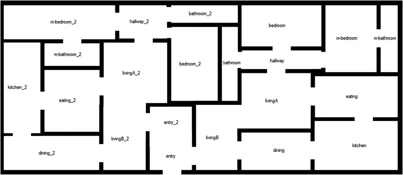
The problem that needs to be solved is to subdivide a given area in such a way that the resulting subareas possess the desired sizes and neighborhood relationships. The subdivision of a surface or a space is usually based on recursive algorithms. The sequence and location of the slicing lines may be stored and organized as a tree structure, a so-called slicing tree, wherein the subareas are represented as a node and the resulting final areas as leaves. This type of data structure can be created, searched, and processed very efficiently, which is why subdivision algorithms are commonly applied in computational geometry, for example, for nearest neighbor queries (Moore, Reference Moore1991).
2.3. EAs
The two methods we propose to study are based on evolutionary strategies (ES), which were elaborated in the 1960s by Bienert, Rechenberg, and Schwefel (Bäck, Reference Bäck1994). In ES, the genotypes are represented by uncoded parameter values (usually in the form of decimal values). The variation through crossover and mutation is directly applied to the parameter values. This obviates the need for decoding and encoding as is, for example, necessary in genetic algorithms (GAs). Consequently, the ES differs from the GA primarily in the way parameter values are represented. The subdivision method combines ES with GA and genetic programming (GP), which traces back to Koza (Reference Koza1992) and is very similar in its functionality to GA; the difference is that in GP not only parameter values but also parts of functions or programs can be represented and combined.
In the formal representation of the EAs, we are guided by Bäck et al. (Reference Bäck, Hoffmeister and Schwefel1991), Bäck (Reference Bäck, Bäck, Fogel and Michalewicz2000), as well as Deb (Reference Deb2001). We restrict ourselves to the main formal elements that characterize ES. ES use P populations of individuals a. The variables µ and λ denote the number of parent and child individuals in a population, and P t = (a t1, … , a tµ) characterizes a population in generation t. When using multiple parents per generation µ > 1, ρ parents can be involved in the production of a child. Accordingly, the notation of ES is as follows: (µ/ρ + λ) – ES.
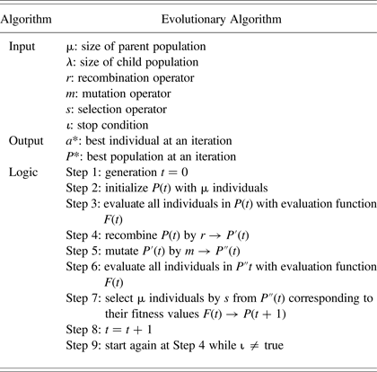
The EA employed share a common structure, which is a cycle that consists of the recombination, the mutation, the evaluation, and the selection of individuals in a population. On its basis, a general process scheme for EA can be built, which is presented in Table 1 and adapted from Bäck (Reference Bäck, Bäck, Fogel and Michalewicz2000).
Table 1. Evolutionary algorithm

Note: The evolutionary algorithm follows Bäck (Reference Bäck, Bäck, Fogel and Michalewicz2000).
3. METHODS
The systems presented in the scope of this paper employ two requirements (constraints) in the generation of the layouts: first, the sizes of the desired rooms, and, second, the topological neighborhood relations between rooms (which rooms need to be adjacent). Based on these two restrictions, a lot of different geometric layout solutions can be generated that meet all requirements.
3.1. Dense packing
The fulfillment of both requirements, correct room sizes and neighborly relationships, poses a multicriteria optimization problem. To solve this multicriteria optimization problem, we employ an implementation suggested by Koenig and Schneider (Reference Koenig and Schneider2012), which can be considered as a combination of the vector evaluated genetic algorithm by Schaffer (Reference Schaffer1985) and the vector-optimized evolution strategy for Kursawe (Reference Kursawe, Schwefel and Männer1990). The corresponding algorithm is described in detail in Koenig and Schneider (Reference Koenig and Schneider2012).
In the following, we describe this procedure of floor plan generation as the dense packing layout solver. It has been extended for the present comparative analysis using more populations in parallel for the solution search. A conservative population was implemented as (+) selection, in which the best variant is always preserved, and several innovative populations are implemented as (,)-selection, in which local optima can be easily overcome. The best solutions of the (,)-selection populations are copied regularly to the (+)-selection population.
3.2. Subdivision
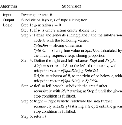
In the scope of the present study, a subdivision algorithm is understood as the recursive division of an area into smaller rectangular areas by edge-parallel slicing. Further subdivisions can be applied to the resulting subareas up to a specified depth or according to a predetermined sequence (Table 2; Otten, Reference Otten1982). The slicing dimension and the subdivision position can be selected and determined randomly or according to fixed rules, for example, that an area is always divided on its longer side and at a fixed proportion ratio, or so that all of the resulting subspaces possess the same area. In the following, this procedure for floor plan generation is referred to as the subdivision layout solver. It is described in full detail in Knecht and Koenig (Reference Knecht, Koenig, Donath, Koenig and Petzold2012) and is reproduced here in abbreviated form (Table 2).
Table 2. Schematic subdivision algorithm and construction of a slicing tree

3.2.1. Calculation of specific room sizes
With the subdivision algorithm, the dividing ratio and split values can be directly calculated on the basis of given room sizes and a given division sequence. Unlike with the dense packing layout solver, optimization is unnecessary in this case. In the scope of the subdivision layout solver, layouts therefore only have to be optimized for one criterion, namely, the objective function of the neighborhood relations.
The calculation of the split values starts at the leaves of the slicing tree. The weight of an area or leaf is calculated out of the ratio of its desired size to the area average. The area average is derived by dividing the total area by the number of rooms. For example, with a total area of 75 m², the area average for six rooms is 12.5 m². In this case, a room with 15 m² has a weighting of 1.2 and a room with 10 m² has a weighting of 0.8. The weighting of a node is calculated out of the sum of the weightings of its two branches, that is, a node to which the two aforementioned rooms are assigned would have a weighting of 2. In this manner, the weightings of all rooms and nodes are defined from the leaves upward to the root (Fig. 1). The corresponding layout is shown in Figure 2.

Fig. 1. Slicing tree: six rooms with (left) sizes and (right) corresponding weightings in leaves and nodes. Syntax: H(V(o)(H(V(o)(o))(o)))(V(o)(o)). Reprinted with permission from Knecht and Koenig (Reference Knecht, Koenig, Donath, Koenig and Petzold2012).

Fig. 2. Subdivision sequence and geometrical ratio in a layout. Syntax: H(V(o)(H(V(o)(o))(o)))(V(o)(o)). Reprinted with permission from Knecht and Koenig (Reference Knecht, Koenig, Donath, Koenig and Petzold2012).
3.2.2. Search for specific neighborhood relationships
Searching for specific neighborhood conditions is a topological problem. It consists of the suitable assignment of functions to rooms and the placement of slicing lines in nodes so that the rooms possess the desired neighbors after subdivision. In contrast to the problem of creating rooms with predefined sizes, we cannot calculate required neighborhood relations directly.
Solutions are searched by using a (µ + λ) – ES in combination with GA and GP. The schematic procedure is shown in Table 2. GA and GP are the basis for the recombination and mutation of the parent individuals in Steps 4 and 5 of the EA.
The GA is used to optimize the allocation of functions and indices to the rooms in terms of required neighborhood relationships. The indices of the rooms are encoded in the sequence as they occur during subdivision. For optimization, this index sequence is mutated and recombined. The sequence is mutated by swapping two indices within the sequence, which corresponds to exchanging the indices of two rooms. In the recombination stage, new variants are created by crossing over index sequences of two individuals using one-point-crossover.
GP is employed to add variation to the structure, that is, the subdivision sequence of a slicing tree. The sequence is mutated by switching the slicing direction in a node from horizontal to vertical or vice versa, or by using crossover. For crossover, we exchange branches between the trees of two parent individuals. The two parents are selected by binary tournament selection. Then, the slicing tree branches to be exchanged are defined, each having the same number of leaves so that the total number of rooms in the child individual remains the same as its parents'. We calculate the fitness function as the sum of all distances between rooms that need to be neighboring as follows:
 $$\,f = \sum\limits_{i = 1}^n {{A_l}{B_l}\comma \; }$$
where A and B represent the rooms which have to be next to each other and n is the number of neighborhoods relations. The distance between two adjacent rooms is zero. Consequently, the unnormalized result of the fitness function is lower when more desired neighborhood relations are fulfilled in a layout or when the corresponding rooms are located more closely together.
4. SCENARIOS
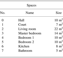
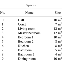
The comparative analyses of the two layout solvers are based on three scenarios. We based the design of the first scenario on a reference layout problem from Flemming et al. (Reference Flemming, Baykan, Coyne, Fox and Gero1992), with its corresponding restrictions. The number and size of the eight rooms of this reference problem are shown in Table 3 and are referred to hereafter as layout scenario 1.
Table 3. Layout scenario 1

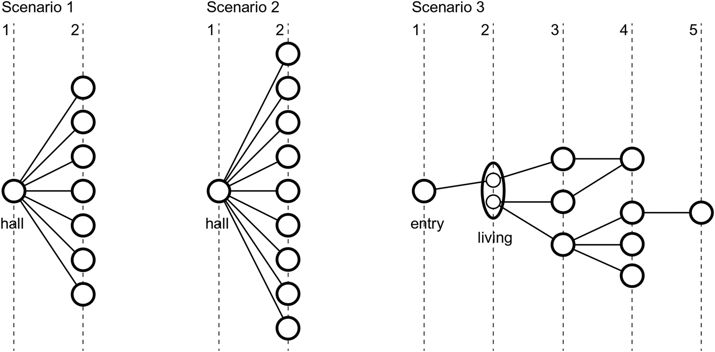
In contrast to the reference problem, we have modified the topological restrictions, because in the scope of our layout solvers we do not provide relations in respect to the cardinal directions. We defined a star topology as topological restriction in both scenarios in which all rooms must be adjacent to a central room (Fig. 3). Because this requirement is relatively difficult to meet compared with the reference problem, we think that our investigations represent a good comparison to the analysis carried out by Flemming et al. (Reference Flemming, Baykan, Coyne, Fox and Gero1992). The smaller number of restrictions used offers, in our view, the advantage that we can use a system that has the minimum of requirements to generate floor plans when comparing two different layout solvers.

Fig. 3. Illustration of the three topologies used for the corresponding three layout scenarios as justified gamma graphs. The nodes represent rooms and the lines connections (doors) between these rooms. The living room in scenario 3 is divided into two subrooms to allow the creation of L-shaped room geometry.
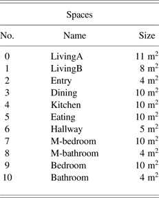
The second scenario extends scenario 1 and is a problem with 10 rooms and the same topological constraints as the first scenario. The room sizes for scenario 2 are given in Table 4. Because two more rooms and connections have to be considered and solved, the second scenario is more difficult to solve than the first.
Table 4. Layout scenario 2

The scenarios considered here are derived from real planning tasks, because it is often possible to reduce more complex tasks to a simpler representation that makes it possible to apply one of the presented layout solvers. In tasks dealing with larger space allocation plans, meaning more rooms to consider than in our test scenarios, functionally related parts are usually defined, which may be related to each other at different hierarchical levels (Koenig & Schneider, Reference Koenig and Schneider2012).
Layout scenario 3 has been chosen to explore the capabilities of our layout solvers when faced with more complex layout generation problems, that is, the generation of L-shaped rooms and the solution of topologies of greater depth and interconnectivity (Fig. 3). Scenario 3 is based on a reference problem defined by Flack and Ross (Reference Flack and Ross2011) to evaluate the capabilities of a system to create advanced floor plans. Table 5 gives an overview of the rooms and their respective sizes. The living room is composed of two subareas to allow for L-shaped spaces, which will be described in more detail in Section 5.6.
Table 5. Layout scenario 3

Figure 3 shows the topologies of the three layout scenarios using a neighborhood graph (Grason, Reference Grason1971). These graphs represent the main goal function for the optimization mechanisms of both layout solvers presented in this paper.
5. COMPARATIVE ANALYSES
In this section, we compare the properties of the layout solvers previously introduced for the production of floor plans using dense packing and subdivision algorithms. The comparison of both systems is based on the layout scenarios described above (Tables 3 and 4). For the application of the developed systems, it is mainly of interest to determine how quickly solutions can be found (performance), how certain one can be that after a specific time span a solution is found (reliability), and how many different solutions can be found in general (variance). In the authors' opinion, these three parameters are suitable for characterizing the most important properties of a layout solver, and they are therefore useful for future comparisons with other solvers.
5.1. Performance
To analyze performance, we proceeded as follows: each layout solver is run 100 times and the quality of the results is recorded in a diagram for the first (Fig. 4) and the second (Fig. 5) layout scenario. This enables us to visualize both the speed with which solutions of a certain quality are obtained on average and the average quality of the solutions within a given time period. Both systems use a (µ/ρ + λ) – ES. Values for the characteristic parameters are µ = 7, λ = 35, ρ = 2, and ρr = 0.75. All calculations for both layout solvers were run on a Dell Precision T7500-2 (Intel Xeon CPU, 2.40 GHz, 48 GB RAM, Windows 7, 64 bit). The diagrams in Figure 4 and Figure 5 show the results of the performance tests. On the top, are the diagrams for the dense packing layout solver, in which on the y axis the sum of all overlapping areas (left ordinate) and all distances (right ordinate) are plotted as fitness values. The mean values of the two fitness values are plotted over the course of 100 recorded generations (or iterations) as mean value lines. The green solid line represents the average values of the overlapping and the blue dotted line represents the mean values of the distances.

Fig. 4. Comparison of the performance of layout scenario 1 (8 rooms). Top: the dense packing layout solver, on the y axis the sum of all overlapping areas, and all distances are plotted as fitness values. Bottom: the subdivision layout solver, the fitness values for neighborhood relations are plotted on the y axis. The x axis shows the number of generations of the evolutionary strategies (ES).

Fig. 5. Comparison of the performance in layout scenario 2 (10 rooms). Top: the dense packing layout solver, on the y axis the sum of all overlapping areas, and all distances are plotted as fitness values. Bottom: the subdivision layout solver, the fitness values for neighborhood relations are plotted on the y axis. The x axis shows the number of generations of the evolutionary strategies (ES).
On the bottom, Figure 4 and Figure 5 show the diagrams for the subdivision layout solver. Because we can calculate the required room sizes directly in this case, we only optimize the layouts with regard to their neighborhood relationships. Consequently, only one criterion has to be optimized in this layout solver. The respective fitness values are plotted on the left y-axis ordinate in the diagrams in Figure 4 and Figure 5, called topology. A value of 0 means that all the neighborhood relations are fully met, and a value of 1 means that the rooms that are to be adjacent to each other are a maximum distance from each other, and consequently none of the requested neighborhood relationships is fulfilled. The red continuous line represents the mean value of the topology fitness over the course of 100 recorded generations.
For layout scenario 1 with the dense packing layout solver, both lines in Figure 4 (top diagram) fall exponentially and reach very good results from about 50 generations onward; after that, the quality of the results improves only marginally. This means that we can assume that the dense packing layout solver finds viable solutions for layout scenario 1 on average after 50 generations. The dense packing layout solver requires on average 27 s for the calculation of 100 generations and 13.5 s for 50 generations accordingly (Table 6). For all time designations, we have to take into account that these represent average values of 100 repeated program runs. The duration of a run increases with time because of the nonoptimized program code, the creation of the performance graphs, and the calculation of the mean value curves in each iteration. A single run of the program is approximately two to three times faster than the averages given here.
Table 6. Overview of calculation times for the dense packing and subdivision layout solvers for both layout scenarios

Note: The calculation times are after 50 and 100 generations. The times for a single run with the dense packing and subdivision layout solvers are given in parentheses.
For layout scenario 1 with the subdivision layout solver, the line in Figure 4 (bottom diagram) falls exponentially and reaches very good results from about 50 generations onward; after that, the quality of the results improves only marginally. This means that we can assume that subdivision layout solver also finds viable solutions on average after 50 generations for layout scenario 1. The calculation of 100 generations takes the system on average 11.5 s and of 50 generations 3.5 s (Table 6). We observed the same effect (a decrease in computing speed over time) for the dense packing layout solver.
The performance tests of both layout solvers for layout scenario 2 are shown in Figure 5 and follow the same concept explained above. The average lines that indicate the average quality of the solutions also fall exponentially for both systems and reach good results from about 50 generations onward, improving only marginally afterward. Therefore, for layout scenario 2, we can also assume that both systems find suitable solutions after an average of 50 generations. The dense packing layout solver requires 44 s for the calculation of 100 generations. The subdivision layout solver needed 12.5 s to calculate 100 generations (Table 6).
5.2. Reliability
This section examines how reliable the considered systems are at finding solutions for the specified layout scenario. To ensure comparability, we take a look at the layouts found by the systems after 100 generations, where both usually converge to one solution, respectively, a local optimum. The point clouds in the diagrams in Figure 4 and Figure 5 show that some runs generate considerably worse results than indicated by the respective mean curves.
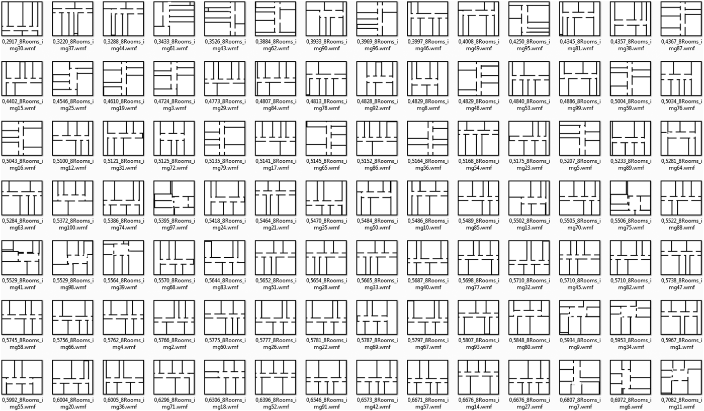
For the dense packing layout solver, solutions are considered to be acceptable when the value of their overlapping areas falls below a certain threshold. This value should be less than 0.1 (normalized value, the dots indicate the overlapping areas) in the scales of the diagrams in Figure 4 and Figure 5. In the diagrams for the dense packing layout solver, we can see that at generation 100 some points are above this threshold: these represent illegal solutions. Figure 6 shows the different layouts, whose qualities regarding their evaluation criteria (overlapping and topology respective adjacency) are represented by the points in the diagrams on the left in Figure 4 and Figure 5. We observed that the dense packing layout solver generates approximately 10% illegal solutions for both layout scenarios. Therefore, it has a reliability of about 90%. The reliability can be increased to nearly 100% by calculating further generations or by increasing the population size. Both options result in longer computing times, which is relevant for user interaction when a system should provide immediate feedback.

Fig. 6. Screenshot of solutions for layout scenario 1 (8 rooms) found by the dense packing layout solver after 100 generations.
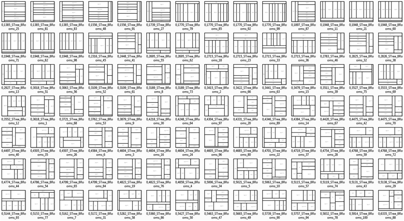
For the subdivision layout solver, solutions are considered to be acceptable if all neighborhood relations are satisfied. The diagrams on the right in Figure 4 and Figure 5 show that the topological requirements are met with a reliability of about 95% on average after 100 generations. We register a small dispersion of the measurement points in the diagrams for the subdivision layout solver at generation 100. Figure 7 shows different layouts generated by the subdivision layout solver, whose properties with regard to the evaluation criteria, that is, how well the topology of the solution matches the required adjacencies, are represented by the points in the diagrams on the right in Figure 4 and Figure 5. We observed that the subdivision layout solver generates approximately 10% illegal solutions for layout scenario 1 and up to 20% illegal solutions for layout scenario 2. Therefore, it has a reliability of about 90% and 80%, respectively.

Fig. 7. Screenshot of solutions for layout scenario 1 (8 rooms) found by the subdivision layout solver after 100 generations.
The discrepancy between the relatively good average fitness value and the reliability of the solution output can be explained by the following characteristic of the layout solver: especially where there are a relatively large number of rooms, such as in layout scenario 2, the system generates solutions that do not completely meet the topological requirements because the defined minimum contact area for the placement of doors cannot be fulfilled for all neighboring rooms.
5.3. Variance
Variance describes the spectrum of different solutions (Rittel, Reference Rittel1992) that can be generated by both systems. The greater the variance, the larger the number of distinct solutions a layout solver can generate. Variance can, therefore, be understood as a measure for the diversity of possible solutions. In a perfect world, we would expect a system for automatic floor plan generation to generate any desired configuration. An overview of the variance of the two compared layout solvers is given in Figure 6 and Figure 7. However, it is difficult to distinguish between the different solutions based on a characteristic value and to formulate a characteristic value for the variance of a system.
For the differentiation of solutions we introduce a proportion parameter θ, which is determined using the following function:
 $${\rm \theta} = \sum\limits_{i = 1}^n {} \left({\displaystyle{{k{S_i}} \over {l{S_i}}}} \right)/{N_{\rm R}}\comma \;$$
where kS i represents the shorter and lS i the longer side of a room and N R the number of rooms. The individual solutions in Figure 6 and Figure 7 are sorted by this proportion parameter. The characteristic values assist in approximately ordering the different solutions. In addition, it could be used as a diversity measure to ensure the variety of an EA's population. However, in some cases, very different solutions have a similar characteristic value. Therefore, for an accurate comparison, a visual inspection is required.
Using the proportion characteristic and comparing the layouts in Figure 6 and Figure 7 visually, it becomes clear that a large proportion of the solutions of the two systems are the same, despite the different properties of the layout solvers used. For example, the subdivision layout solver only finds solutions in which at least one continuous wall exists from one to the other outer side of the enclosing rectangle. As we can see in Figure 6, the dense packing layout solver also rarely generates layouts where this is not the case, at least for the star topology. However, there are layout solutions that are predominantly found only by one of the two systems. For instance, the subdivision layout solver generates a relatively uncommon layout in which the central room (hall) of the star topology with the most connections (doors) to other rooms is arranged on the outer wall. This variant is extremely rare for the dense packing layout solver and does not occur in the solution set shown in Figure 6.
As a simple parameter for the variance ν of a system, we use the difference between maximum and minimum proportion characteristics of θ of a solution set of 100 individual solutions:
In a set of 100 solutions, the dense packing layout solver shows a variance ν8 = 0.52 for 8 rooms and ν10 = 0.44 for 10 rooms. For the subdivision layout solver, the corresponding variances are ν8 = 0.52 and ν10 = 0.45. The values for variance ν may vary slightly from the specified values dependent on the individual run.
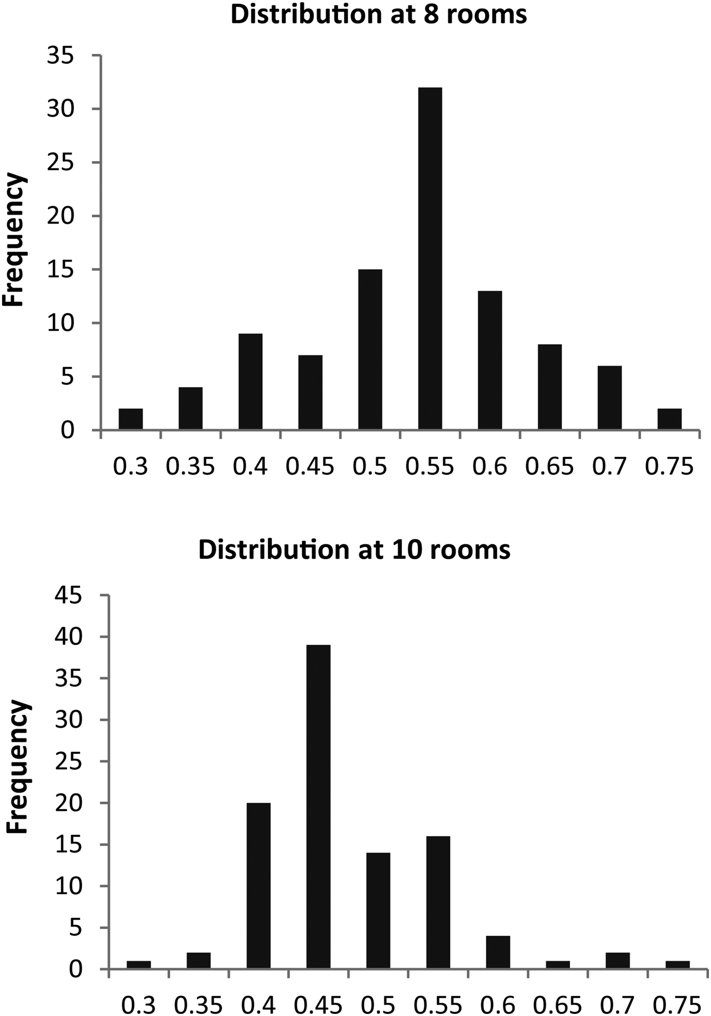
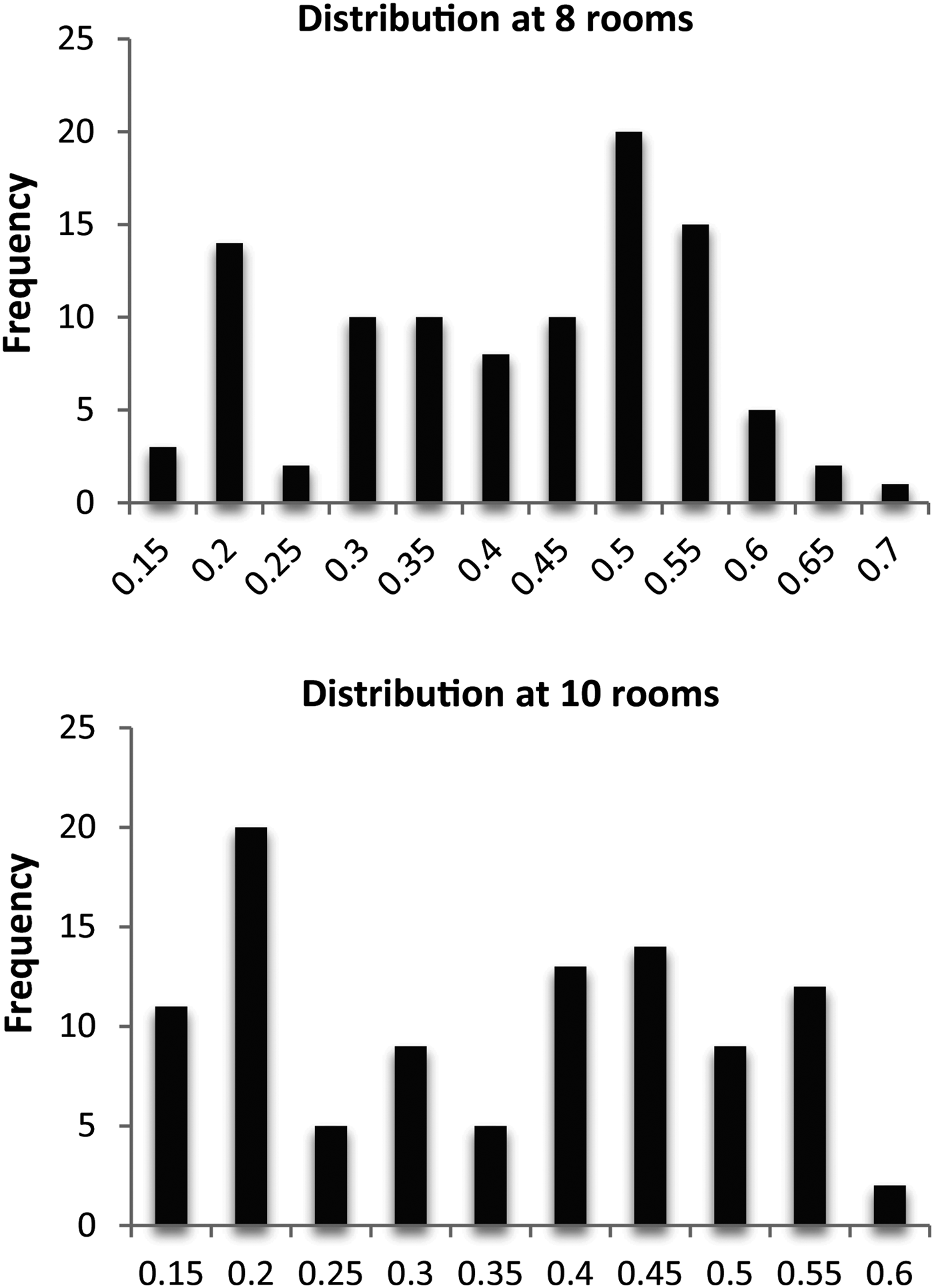
Besides the illustrated characteristic value for the variance ν of a system, the distribution of the proportion parameters is of interest. It gives us an idea about the probability with which certain variants are generated, and whether the layout solver tends to find solutions within a certain proportion parameter area. Our goal is a system that can generate solution sets with the largest possible variance with a uniform distribution of the proportion parameters.
The histograms in Figure 8 and Figure 9 show the corresponding distributions of proportion parameters for 100 generated layouts for both systems. In the diagrams for the dense packing layout solver in Figure 8, we can see clearly that the proportion parameter values accumulate strongly in a particular area and that the distribution of the values tends to a normal distribution. This means that the system has a preference to generate specific configurations (Fig. 6). The diagram for the subdivision layout solver in Figure 9 shows that the proportion parameters are spread relatively evenly across the entire variance spectrum. The subdivision solver seems to have no strong tendency for certain configurations; only the upper proportion characteristics are less common.

Fig. 8. Histograms of proportion parameters for the dense packing layout solver after 100 generations and a set of 100 solutions. Top: for 8 rooms; bottom: for 10 rooms. The y-axis values are for proportion parameter θ, and the x-axis values are the number of solutions in the θ range.

Fig. 9. Histograms of proportion parameters for the subdivision layout solver after 100 generations and a set of 100 solutions. Top: for 8 rooms; bottom: for 10 rooms. The y-axis values are for proportion parameter θ, and the x-axis values are the number of solutions in the θ range.
5.4. Evaluation
The performance of the subdivision layout solver is better compared to that of the dense packing layout solver because it generates solutions many times faster. The quality of the generated solutions and the reliability of both systems are roughly equal. In addition, the variance of both systems can be considered equally strong. Both layout solvers are able to find all possible configurations with a few exceptions only, as mentioned above. Comparing the distribution of proportion characteristic values, the subdivision layout solver provides advantageous results, because the characteristic values of the solutions generated by this layout solver are distributed relatively evenly and configurations do not occur in clusters. This means that the subdivision layout solver explores the solutions space in all areas relatively equally, which is ideal, for example, if we were to add further restrictions or goal functions for even more complex scenarios.
5.5. Interaction characteristics
The two layout solvers differ primarily in the way one can interact with individual elements of the layout. The interaction possibilities depend on the characteristics of the algorithms used. The subdivision algorithm allows only line-based interaction. This means that the walls of a layout can be moved, the graphical displacement of a room border by s thus resulting in the displacement of the splitting line by distance s. Consequently, one can primarily change the room sizes through interaction. A problem is that long splitting lines cannot be divided, that is, moving one line changes the borders and therefore also the sizes of several rooms. However, in this system one cannot directly manipulate the positions of individual rooms. This characteristic makes it hard to predefine the placement of certain rooms, such as stairwells, precisely above each other in multistory building layouts and to fix them within the layout.
In contrast, the dense packing layout solver does permit additional room-based interaction, which offers more extensive possibilities than the line-based one. In addition to the adjustment of room sizes through the manipulation of boundary lines, individual rooms can be displaced within the layout and fixed in their position. This makes it possible to realize precise vertical spatial alignments as well as links to higher hierarchy levels.
5.6. More complex layouts
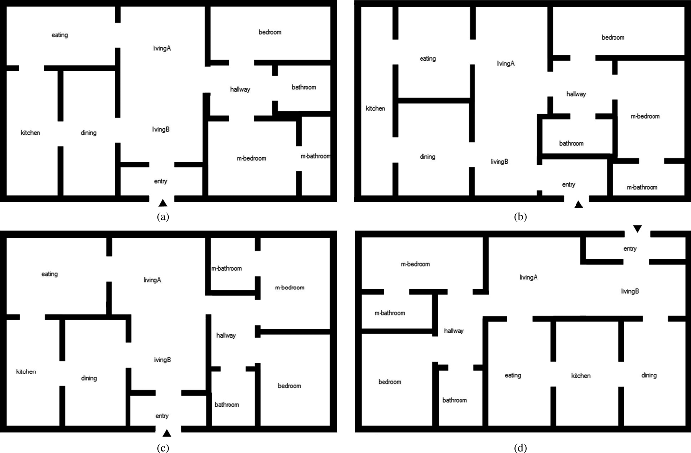
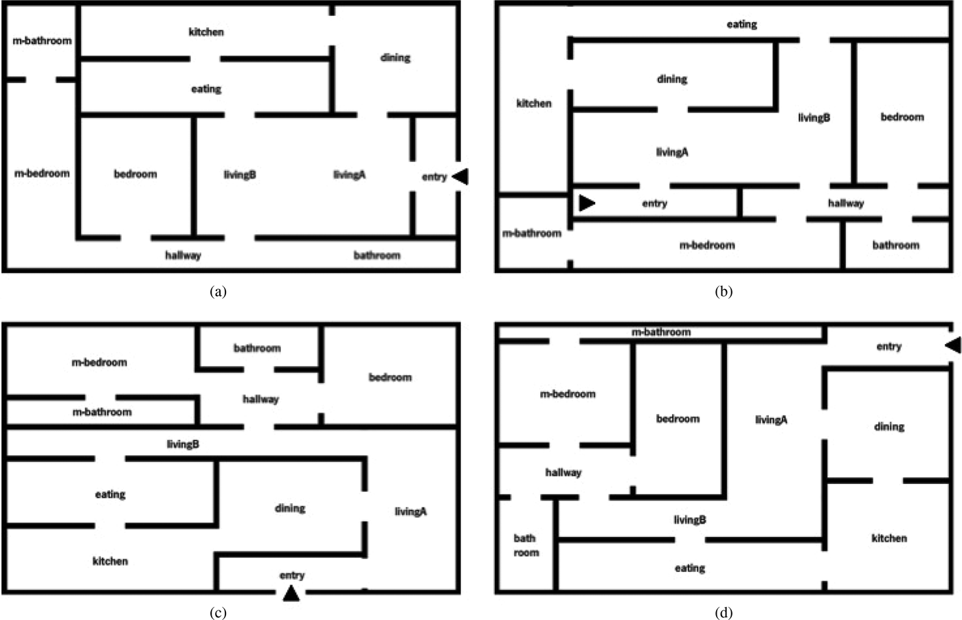
To prove that we can generate other, more complex layouts with both layout solvers, we introduced layout scenario 3 (Fig. 3 and Table 5). The room topology of this scenario has a higher depth (=5) compared with the first two scenarios (depth = 2). The primary intention, however, is to show the possibility of creating L-shape rooms by removing a joint wall between two adjacent rooms. We therefore decomposed the living room into two subareas (livingA and livingB) in layout scenario 3 and connected them appropriately. The results generated by the dense packing layout solver are illustrated in Figure 10, those of the subdivision layout solver in Figure 11. The dense packing layout solver requires on average 24 s for the calculation of 100 generations and 12 s for 50 generations, and the subdivision layout solver requires on average 20 s for the calculation of 100 generations and 9.5 s for 50 generations (Table 6). We can see that the decomposition of one large room does not necessarily result in L-shaped rooms (Figs. 10a, 11a). This layout scenario shows that it is possible to generate quite different kinds of floor plans. The decomposition method (for combined rooms, e.g., L-shaped ones) is also useful for the generation of long branched corridors in complex buildings, but it is more efficient to represent very complex layout scenarios in a hierarchical way (Koenig & Schneider, Reference Koenig and Schneider2012).

Fig. 10. Screenshot of four solutions for layout scenario 3 (11 rooms) found using the dense packing layout solver.

Fig. 11. Screenshot of four solutions for layout scenario 3 (11 rooms) generated by the subdivision layout solver.
To show that using evolutionary optimization techniques for the presented layout solver can solve problems with as many as 22 rooms, we undertook the same test using two layout scenarios 3 and coupled the individual graphs via their entry rooms. Figure 12 shows a solution generated with the dense packing layout solver. For this solution the solver needs approximately 50 s, which makes useful user interaction no longer practicable.

Fig. 12. Screenshot of a solution for two layout scenarios 3 (22 rooms) coupled via their entry rooms generated by the dense packing layout solver.
6. CONCLUSION AND OUTLOOK
In this article, we presented dense packing and subdivision algorithms as two evolutionary algorithm based methods for rectangular architectural layout generation and compared the two respective layout solvers with respect to their performance, that is, the speed with which they find possible solutions, their reliability in finding suitable solutions, and the variance of their solutions found. Both systems represent practical solutions for the automatic creation of floor plans in the context of complex planning processes. The differences are mainly in detail. The subdivision layout solver has better performance, while the dense packing layout solver is better suited for user interaction. The variance of both systems is comparable. This property is essential in order to ensure that a large number of different layouts can be generated, which may then be refined by applying other constraints.
We compared the two layout solvers based on three different layout scenarios. Scenario 1 was based on a reference scenario defined by Flemming et al. (Reference Flemming, Baykan, Coyne, Fox and Gero1992), and a comparison of the performance of our two layout solvers shows the following: at first glance, the performance of the layout solvers we present here is better because a single solution is found in about 4 s. However, Flemming et al.'s systems are more than 20 years old, and their fastest solver required 12 s for the solution of a comparable layout scenario. It is likely that the performance of this system would achieve much better results on a contemporary machine.
The method we present here for dealing with more rooms with more complex geometry is based on the explicit representation of subareas. This means a designer has to decide in advance which space needs to be more complex or flexible. In principle, this is not a huge problem, because complex spaces are usually needed for special rooms like corridors, entrance halls, and living rooms, which are known from the planning program. However, for a generally applicable layout algorithm, it would be more convenient to generate complex space geometries automatically as needed. We therefore need to extend the genetic representation for the geometry, although this has the disadvantage that the search space for the optimization system increases and with this the time needed to find good solutions.
In future developments of the floor plan layout system, we plan to extend it to cover as many criteria as possible for multicriteria optimization as exemplified by Flack and Ross (Reference Flack and Ross2011). As mentioned, more fitness criteria will probably require a more complex chromosome structure, resulting in larger search spaces and higher computing times. One of the central aspects in developing successful layout systems is how to find a good compromise that offers designers usable and useful user interaction while still making it possible to optimize as many criteria as possible.
ACKNOWLEDGMENTS
This project was undertaken primarily at Bauhaus-University Weimar and funded by the German Research Council under Funding Number DO 551/19-1. One author was supported by the Media and Arts Technology program, which is funded by UK Research Councils. Many thanks to Julian Reisenberger for the language editing.
Reinhard Koenig is a Senior Assistant and Lecturer at ETH Zurich and has worked as a Research Assistant and Interim Professor at Bauhaus-University Weimar. He completed his PhD thesis in 2009 at the University of Karlsruhe, and he studied architecture and urban planning. He heads research projects on the complexity of urban systems and societies, the understanding of cities by means of agent-based models and cellular automata, as well as the development of evolutionary design methods. Dr. Koenig's current research interests are the applicability of multicriteria optimization techniques for planning problems and correlations of computed measures of spatial configurations with human cognition and usage of space.
Katja Knecht is a Researcher and Designer with a background in media technology and architecture. After graduating from the Bauhaus-University Weimar with a master of science degree in media architecture in 2011, she worked as a Research Assistant at the Chair of Computer Science in Architecture. In 2012 she joined Queen Mary University of London to pursue a PhD in the Media and Arts Technology Programme. Her research is cross-disciplinary and situated at the interface among architecture, media, and computing. The range of Ms. Knecht's work is from the development of generative and media-based tools to support architectural design and work processes to the creation of tangible environments and mediated spatial experiences.

