4.1. Example of an optical lens system

To aid in explaining optical prescriptions, Figure 1 shows a system (Smith, Reference Smith2000, p. 508) composed of four spherical lenses intended for use as a telescope eyepiece. Tackaberry and Muller patented this lens system in 1958 (Tackaberry & Muller, Reference Tackaberry and Muller1958), and is an improved design within a subclass of the Konig lens systems patented in 1940 (Konig, Reference Konig1940). In this optical lens system, the OBJ is shown at the far left of the figure and the IMS is shown at the far right. Curved surfaces 1 and 2 together define the first lens. Surfaces 3 and 4 together define the second lens. Curved surfaces 5, 6, and 7 together define a doublet (i.e., two lenses fitting snuggly together). Light rays a, b, and c (so-called axial rays) start at the OBJ (at the far left), enter the system in parallel at the entry pupil (EP), and eventually converge (at the far right) to a single point (focal point f) on the IMS. Light ray d (so-called chief ray) starts from the point farthest from the axis on the OBJ plane that is visible through the lens system (FOV). This chief ray runs through the center, e, of the aperture stop (EP here) and to the IMS (at a point q, called the image height).

Fig. 1. The Tackaberry–Muller lens system.

4.2. Example of a prescription (lens file)

Table 1 shows a prescription (slightly modified for tutorial purposes) for the Tackaberry–Muller lens system (a telescope eyepiece) of Figure 1. Each row in the table represents a surface. The OBJ appears in the first row, the EP appears in the second row, and the IMS appears in the last row. The other surfaces are consecutively numbered (from 1 to 7). All entries in this table are normalized so that the system has a focal length of 1. As will be seen, a single lens is defined by two surfaces having a material, such as glass, between them.

Table 1. Lens file for the patented Tackaberry–Muller lens system

Some of the information on a given row in a prescription pertains to the surface, whereas other information pertains to the space between the surface and the next surface. For example, in Table 1, the radius of curvature of the surface (column 3) and the aperture (column 5) are characteristics of the surface itself. The distance (column 2) refers to the distance between the surface represented by that row and the surface represented by the next row (i.e., the surface to the right). Similarly, the material (column 4) refers to the material (e.g., air, vacuum, glass, polymer, oil, other material) between the surface represented by that row and the surface represented by the next row.

The Tackaberry lens system has an EP. The distance between the OBJ and the EP is infinite (represented here by the value of 10¹⁰). The EP is a flat opaque surface with a small circular hole of semidiameter 0.18 mm, centered at the axis line.

Surface 1 in Table 1 is located at a distance (column 2) of 0.88 from the previous surface (i.e., EP). The value of −3.52361 (column 3) for the radius of curvature of surface 1 indicates that surface 1 is a sector of a sphere with a radius 3.52361. The negative sign indicates that the sphere's center is located to the surface's left. The material (column 4) located to the right of surface 1 is BK7, a commercially available crown glass. The aperture semidiameters for surfaces 1 through 7 (found in column 5) have a uniform value of 0.62 for this particular lens system (a telescope eyepiece).

Surface 2 is located at distance 0.21900 from surface 1. The negative sign of the radius of curvature of surface 2 (−1.05274) indicates that the sphere's center is located to the surface's left. The material to the right of surface 2 is air. Together, surfaces 1 and 2 define a lens of thickness 0.21900 composed of BK7 glass with a concave left surface and a convex right surface. As can be seen in Figure 1, the leftmost surface of this lens is concave and its rightmost surface is convex. Note that surface 2's radius of curvature (1.05274) is smaller than that of surface 1 (3.52361), giving surface 2 a greater curvature.

Surfaces 3 and 4 together specify a lens (composed of BK7 glass) at distance 0.07280 from surface 2 with a concave left surface and a convex right surface.

Surfaces 5, 6, and 7 together define a doublet lens. The material to the right of surface 5 is BK7 glass and the material to the right of surface 6 is SF61, a commercially available flint glass. The positive radius of surface 5 (1.02491) and the negative radius of surface 6 (−0.93493) indicate that the left lens of the doublet is biconvex. The negative radius of surface 6 (−0.93493) and the positive radius of surface 7 (7.94281) indicate that the right lens of the doublet is biconcave. The relatively large (absolute) value of the radius of surface 7 (7.94281) means that surface 7 is almost flat.

The material between surface 7 and the IMS is air and its distance is 0.47485 (the back focal length).

The distance of 0.88 between the EP and surface 1 defines the eye relief of the eyepiece. Eye relief describes the distance between the eye and the eyepiece lens and is an important design criterion of eyepieces. Eye relief (from the perspective of design constraints) is determined by the FOV and the aperture of the EP. In general, the design tradeoff is that the smaller the aperture of the EP and/or the larger the FOV, the shorter the eye relief. This system here has a half FOV (HFOV) of 19.8°.

The format of lens files used in modern-day optical simulation software can accommodate many complex features not illustrated by the above prescription. For example, the surfaces need not be spherical. Instead, an aspherical surface can be specified by a higher order polynomial or even an arbitrary mathematical function. Such aspherical lenses are becoming increasingly common today because it is now possible to manufacture them economically. Another example of a feature not illustrated by the above prescription is that surfaces can be reflective as well as refractive, thereby permitting light rays to travel in nonsequential paths (not just left to right). In addition, it is possible for a surface to consist of multiple subsurfaces containing various geometric shapes (e.g., circular, polygonal) residing at various physical locations on the surface.

4.3. Analysis of an optical system

Once a classical optical system is specified by means of its prescription (lens file), many of its optical properties can be calculated by tracing the paths of light rays of various wavelengths through the system. Ray-tracing analysis is extremely tedious when performed by hand. Today it is typically performed by optical simulation software. Numerous commercial software packages (e.g., OSLO, Zemax, Code V) and public domain software packages (e.g., KOJAC) are available in the field of optical engineering to aid in this process.

Modern optical simulation software yields a multiplicity of curves describing the system's optical characteristics. For example, Figure 2 shows conventional curves for distortion (Fig. 2a), astigmatism (Fig. 2b), chromatic aberration (Fig. 2c), and spherical aberration (Fig. 2d) for the Tackaberry–Muller system (Fig. 1).

Fig. 2. Characteristics of the Tackaberry–Muller system.

Figure 3 shows the on-axis ray intercept diagram (Fig. 3a), a partial field ray intercept diagram (Fig. 3b), and the full field ray intercept diagram (Fig. 3c). Within each subfigure, the diagram for the meridional plane (i.e., planes that contain the optical axis and axial rays) is on the left, with the sagittal plane (i.e., skew planes that contain off-axis rays such as the chief ray) on the right.

Fig. 3. Additional characteristics of the Tackaberry–Muller system.

5.1. Practical limitations on numerical values

When applying genetic programming to a design problem in a particular field, practical considerations usually dictate certain limitations on the range of numeric values that are allowed. In the field of optical design, for example, there is a practical limitation on the radius of curvature of a lens surface and the distance between surfaces. For this work, where the focal lengths of the target systems were normalized to 1 mm, the minimum radius of curvature is −15 and the maximum is +15. The maximum thickness (for glass or air) is 1.0 mm. The minimum thickness for air is 0.01 mm and the minimum thickness for glass is 0.1 mm. The minimum aperture is 0.1 mm (where an opaque mounting is added to cradle a lens that would otherwise be hovering in air). The aspheric coefficient terms have a range from −10 to +10 (for optical systems normalized to a focal length of 1).

5.2. Glass mutation operation

The numerical parameter values for distance and the radius of curvature of a lens can each be established using the standard technique of perturbable numerical values. These perturbable numerical values are perturbed during the run using the standard method in genetic programming for numerical parameter mutation. In this standard method, each perturbable numerical value is set, individually and separately, to a random value in a chosen range in the initial generation of a run (generation 0). After generation 0, the perturbable numerical value may be perturbed. The perturbation is usually relatively small. The value to be perturbed is considered to be the mean of a Gaussian distribution. A relatively small preset parameter establishes the standard deviation of the Gaussian distribution. The value to be perturbed is then perturbed by an amount determined by the Gaussian distribution.

However, the standard method for perturbing numerical values cannot be readily used when mutating materials (e.g., types of glass). In optical design, each type of material is characterized by a set of wavelength-dependent indices of refraction, its Abbe number, and its cost. The Abbe numbers and indices of refraction are interrelated, and therefore cannot be independently varied with total freedom. The 199 commercially available glasses in the Schott catalog reside in a relatively small and compact crescent-shaped area occupying only about 27% of the area of the rectangle bounded by the extreme values of n and V for the catalog, namely, 1.46 < n < 2.02 and 20 < V < 77. The optical designer usually cannot freely choose numerical values for the materials to be used, but must, instead, limit the choices to the relatively small number of commercially available types of materials. This limitation is not just a matter of the higher cost of manufacturing a custom type of glass because it may not be possible to manufacture a type of glass with an arbitrarily chosen Abbe number and a set of arbitrarily chosen indices of refraction for particular wavelengths. Accordingly, our mutation operation for materials changes one type of material in the chosen catalog to another type of material in the catalog whose properties are nearby in the multidimensional space of properties.

5.3. Toroidal mutation operation for the radius of curvature

A flat surface can be viewed as a spherical surface with a very large positive or negative radius of curvature. That is, a very large positive or negative radius represents the same thing. Thus, it is advantageous to slightly modify the standard method used in genetic programming for numerical parameter mutation when perturbing the radius of curvature. Accordingly, our numerical parameter mutation operation for curvatures operates in a toroidal way (wrapping +15 to −15) when it is applied to a terminal representing the radius of curvature.

5.4. Lens splitting operation

A lens-splitting operation appears to be useful for the field of optical design. The lens-splitting operation is performed on a single parent selected probabilistically from the population based on its fitness. The lens-splitting operation replaces one randomly picked lens with two new lenses. Figure 4 shows an illustrative lens system, and Figure 5 shows the result of applying the lens-splitting operation. The thickness of each of the two new lenses is half of the thickness of the original lens. The radius of curvature of the first surface of the first new lens is set equal to the radius of curvature of the first surface of the original lens. The second surface of the first new lens (which is the same as the first surface of the second new lens) is flat. The radius of curvature of the second surface of the second new lens is set equal to the radius of curvature of the second surface of the original lens. When the original lens is a single lens (as is the case in Fig. 5), the result of the lens splitting operation is a doublet lens (as shown in Fig. 5). The lens-splitting operation is intended to be optically neutral (and, hence, does not change the fitness of the lens system involved). The one exception occurs if half of the thickness is less than the minimum permissible lens thickness. In that event, the thickness of each new lens is set to the minimum (and the overall length of the lens system is slightly increased). Note that because of the toroidal behavior of the numerical parameter mutation operation, the newly created flat surface has an equal probability of being perturbed to a negative or positive radius of curvature when it is first mutated.

Fig. 4. Lens system before lens-splitting operation.

Fig. 5. Lens system after lens-splitting operation.

The motivation for the lens-splitting operation is that the insertion of additional surfaces or lenses by means of crossover rarely yields an improved individual. The lens-splitting operation creates an offspring that almost always has the same (reasonably good) fitness as its parent. It thus introduces topological diversity without changing fitness. Subsequent glass mutations or numerical mutations of the distance or radius of curvature can then be done gradually.

7.1. Function Set

The first preparatory step in applying genetic programming involves identifying the function set for the programs to be evolved. The same function set is used for all the problems presented in this paper.

The widely used and well-established format for optical prescriptions (and lens files for optical analysis software) suggests a developmental process suitable for representing optical lens systems. This developmental representation employs a “turtle” similar to that used in Lindenmayer systems (Lindenmayer, 1968; Prusinkiewicz & Lindenmayer, 1990). A turtle was used in our previous work in synthesizing geometric patterns using developmental genetic programming (Koza, 1993) and in synthesizing antennas using developmental genetic programming (Comisky, Yu, & Koza, Reference Comisky, Yu and Koza2000; Koza, Keane, Streeter, Mydlowec, Yu, & Lanza, 2003a).

In our developmental representation for optical lens systems, the turtle starts at the point where the system's main axis intersects with the EP surface (point g in Fig. 6) and inserts optical surfaces and materials as it moves. The distance between point g and point e (where the EP surface intersects the system's main axis b) defines the eye relief of the system. Figure 6 shows the beginnings of the Tackaberry–Muller lens system shown of Figure 1 (where the eye relief is 0.88 mm).

Fig. 6. Turtle starts at point g along main axis b.

The function set

contains two functions

The three-argument spherical surface (

) function causes the turtle to do three things at its starting point (and each subsequent point to which the turtle moves). First, it inserts a spherical surface with a specified radius of curvature at the turtle's present location. Second, the

function moves the turtle to the right by a specified distance along the system's main axis. Third, the

function fills the space to the right of the just-added surface with a specified type of material (e.g., air, vacuum, glass, polymer, oil, other material).

Radius and distance values are each established by a value-setting subtree of the

function consisting of a single perturbable numerical value.

The material is established by a value-setting subtree of the

function consisting of a single terminal identifying the type of material.

The two-argument

function is a connective (glue) function that first executes its first argument and then executes its second argument. It does not itself add anything to the developing structure.

Figure 7 shows the result of the insertion of spherical surface 1 (with a radius of curvature of −3.52361). After inserting this surface, the turtle moves the specified distance of 0.219 from its starting point g to point h along axis line b. BK7 indicates that glass type BK7 (a commercially available crown glass) will be used to fill the space between g and whatever surface is subsequently inserted at point h (by the turtle's next step). These actions by the turtle reflect the information contained on the row labeled surface 1 in the prescription of Table 1.

Fig. 7. Turtle inserts surface 1.

Figure 8 shows the result of the insertion by the turtle of spherical surface 2 (with a radius of curvature of −1.05274). After inserting this surface, the turtle moves the specified distance of 0.07280 from point h to i. Surfaces 1 and 2 together define a lens of thickness 0.219 of BK7 glass. Because the centers of the two spheres defining surfaces 1 and 2 are both positioned in the negative direction (i.e., to the left) along the axis b, this first lens has a concave left surface and a convex right surface. Note that the material inserted to the right of surface 2 is air. That is, air will be used to fill the space between h and whatever surface is subsequently inserted at point i (by the turtle's next step). These actions by the turtle reflect the row labeled surface 2 in the prescription in Table 1.

Fig. 8. Turtle inserts surface 2, thereby completing the first lens.

In a similar manner, the rows labeled surfaces 3 and 4 in the prescription of Table 1 correspond to a second lens of BK7 glass (as shown in Fig. 9).

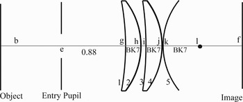
Fig. 9. Turtle inserts surface 5.

Figure 9 also shows the result of the insertion by the turtle of spherical surface 5 (with a radius of curvature of 1.02491). The turtle moves a distance of 0.52100 from point k to l. BK7 glass will be used to fill the space between k and whatever surface is subsequently inserted at point l (by the turtle's next step). These actions by the turtle reflect the row labeled surface 5 in the prescription of Table 1.

Figure 10 shows the result of the insertion by the turtle of spherical surface 6 (with a radius of curvature of −0.93493). The turtle moves a distance of 0.11800 from point l to m. SF4 glass is used to fill the space between l and whatever surface is subsequently inserted at point m (by the turtle's next step). Surfaces 5 and 6 together define a lens of thickness 0.52100 of BK7 glass. The positive radius of surface 5 and the negative radius of surface 6 together indicate that the third lens is biconvex. These actions by the turtle reflect the row labeled surface 6 in the prescription of Table 1. Note that a pair of snuggly fitting lens is being formed by this step because glass, as opposed to air, is filling the space between points l and m. These actions by the turtle reflect the row labeled surface 6 in the prescription of Table 1.

Fig. 10. Turtle inserts surface 6, thereby completing third lens.

Figure 11 shows the result of the insertion by the turtle of spherical surface 7 (with a radius of curvature of 7.94281). Air is used to fill the space between m and whatever surface may be subsequently inserted. The turtle moves a distance of 0.47485 starting from point m. Surfaces 6 and 7 together define a lens of thickness 0.11800 of SF4 glass. Because there was no air between the third lens and this new lens, a doublet is formed. The negative radius of surface 6 and the positive radius of surface 7 together indicate that the right lens of the doublet is biconcave. These actions by the turtle reflect the row labeled surface 7 in the prescription of Table 1. Because there are no additional surfaces in the prescription, the developmental process ends at this stage. The IMS is automatically inserted where the turtle is now located (i.e., at distance 0.47485 from point m).

Fig. 11. Turtle inserts surface 7, thereby completing the forth lens (and creating a doublet).

7.2. Terminal Set

The second preparatory step in applying genetic programming involves identifying the terminal set for the programs to be evolved. The same terminal set is used for all the problems presented in this paper.

The terminal set for each value-setting subtree that establishes thickness or radius values (T _perturbable) is

where ℜ denotes perturbable numerical values between 0.0 and 1.0. The value produced by the value-setting subtree is interpreted using a scale that is appropriate for whether the terminal is being used for a surface's thickness or a radius of curvature.

The terminal set for each value-setting subtree that establishes the type of material (T _material) consists of the names of all of the permissible materials.

A constrained syntactic structure specifies how the functions and terminals may be combined in a program tree. A constrained syntactic structure consists of a set of rules of construction (Koza, Reference Koza1992). The constrained syntactic structure here enforces the occurrence of

• • a

  PROGN2
  function at the top of the program tree (because an optical system consisting of just one surface is of no interest),

• • either an

  SS
  or
  PROGN2
  function as the arguments of the
  PROGN2
  function,

• • a single perturbable numerical value for the value-setting subtree that establishes the radius of curvature (i.e., first argument of the

  SS
  function),

• • a single perturbable numerical value for the value-setting subtree that establishes the numerical value for distance (i.e., second argument of the

  SS
  function), and

• • a single type of material for the value-setting subtree that establishes material (i.e., third argument of the

  SS
  function).

A given optical lens system can be represented in four equivalent ways. Each representation is useful in some aspect of this paper's discussion of how to apply genetic programming to the design of optical lens systems.

First, there is the schematic diagram of the physical lens system (such as shown in Fig. 1). This representation provides a visual picture of the physical lens system.

Second, there is the prescription or lens file (such as shown in Table 1). This representation corresponds to the traditional way by which a lens system is described as a table of numerical and nonnumerical parameter values.

Third, there is the program tree consisting of a composition of functions and terminals. Figure 12 shows a program tree that represents the first two lenses (four surfaces) of the Tackaberry–Muller lens system of Figure 1 and Table 1. Genetic programming operates on a population of program trees.

Fig. 12. Program tree for first two lenses of Tackaberry–Muller lens system.

Fourth, using the LISP programming language, there is the symbolic expression (S-expression) consisting of a composition of functions and terminals. Of the four equivalent representations, the S-expression is closest to the representation used internally by the computer code that implements genetic programming. The S-expression corresponding to the program tree of Figure 12 is shown in the following:

7.3. Fitness measure

The third preparatory step in applying genetic programming to a problem involves constructing the fitness measure. The purpose of the fitness measure is to specify what the human wants. Specifically, the fitness measure must establish a partial order among any two candidate lens systems that may be encountered during the run of genetic programming (i.e., the fitness measure must enable two candidates to be compared so that one is identified as being better than the other). The fitness measures for each of the problems presented in this paper are based on the level of performance of the lens system described in the particular patent. The fitness measures for each of the problems in this paper have the same general structure.

Figure 13 shows the steps in ascertaining the fitness of an individual program tree that may be encountered during the run of genetic programming. When developmental genetic programming it used, the ascertainment of fitness begins with the developmental process. First, the functions in the program tree are executed and applied to an optical embryo to create an optical lens system (as will be explained in additional detail momentarily). Second, the resulting optical lens system is reexpressed as a prescription (lens file) specifying the numerical and nonnumerical parameters associated with each surface in the lens system. Third, the prescription (lens file) is fed into a simulator to obtain the optical behavior and characteristics of the lens system. Fourth, a value of fitness is calculated from the system's behavior and characteristics.

Fig. 13. Steps for ascertaining the fitness of an individual program tree.

Once a classical optical system is specified by means of its prescription (lens file), many of its optical properties can be calculated by tracing the path of light rays of various wavelengths through the system. The ray tracing analysis yields a set of characteristics of interest to optical designers, including distortion, astigmatism, and chromatic aberration. Ray-tracing analysis by hand is extremely time consuming. Ray tracing is typically performed nowadays by optical simulation software (e.g., OSLO, Zemax, Code V, KOJAC). KOJAC is a public-domain educational software package for optical ray tracing originally authored by Olivier Scherler and currently maintained by Olivier Ripoll. We developed our own lens analysis simulator based on KOJAC to evaluate the performance of candidate lens systems. We wrote code to use the ray traces produced by KOJAC to compute relevant optical characteristics, and in addition, wrote our own code for the image analysis. We embedded all of this code in our genetic programming system operating on our Beowulf-style parallel cluster computer. We used a commercially available software package (OSLO from Lambda Research) running on a single workstation for postrun validation of the final results obtained from the cluster computer.

Fitness is measured by embedding each candidate lens system into a fixed structure called the test fixture. The OBJ, IMS, and EP lines of the prescription together constitute the test fixture for evaluating a particular candidate lens system. For the eyepieces discussed in this paper, the distance between the OBJ surface and the EP in the test fixture is fixed at infinity. The distance between the EP and the first surface (eye relief) is fixed for each particular problem and appears as the distance on the line for the EP in the prescription (e.g., the eye relief is 0.88 mm in Table 1). The concept of test fixture used in this paper for optical systems is directly analogous to the test fixture used in connection with the automatic synthesis of electrical circuits by means of genetic programming (Koza, Bennett, Andre, & Keane, 1999; Koza, Keane, Streeter, Mydlowec, Yu, & Lanza, Reference Koza, Keane, Streeter, Mydlowec, Yu and Lanza2003).

The representation scheme used in this paper for applying genetic programming to the field of optical design is similar to that encountered in numerous other fields of design in that it permits the creation of various types of pathological structures that are of no practical interest. In the course of discussing the fitness measure below, we describe how we heavily penalize, slightly penalize, or repair various pathological structures.

The fitness measure is, for practical design problems in most fields, multiobjective in the sense that it combines two or more different elements. Trade-offs between multiple competing considerations are common to most fields of engineering design, regardless of whether the design is being accomplished by evolutionary search, other types of search, or human design. The different elements of the fitness measure are typically in competition with one another to some degree. This is indeed the case for optical design.

Because of the multiple conflicting objectives inherent in problems of optical design, the fitness measure is divided into four distinct phases. Broadly speaking, the four phases sequentially consider whether

• • the system is not degenerate;

• • the system's paraxial aberration performance is at least as good as that of the target (patented) system;

• • the system's image-forming quality is at least as good as that of the target (patented) system; and

• • the system is parsimonious, that is, it has the same or fewer lenses as the target (patented) system.

Numerical and Boolean values are both computed for each of the four phases. That is, fitness is a vector of eight items. The numerical value is used to rank the goodness of a candidate individual. The Boolean value indicates whether the individual satisfies certain minimum performance requirements specified for the phase. In comparing two individuals, an individual satisfying the minimum requirements of a phase (i.e., has a positive Boolean value) is considered superior to any individual that does not. In addition, an individual with a lower numerical value for a particular phase is considered superior to an individual with a higher numerical value for that phase.

To conserve computer time, the fitness evaluation of an individual not satisfying the minimum requirements of a particular phase (i.e., has a negative Boolean value) is short circuited (i.e., simply not evaluated in later phases).

As will be seen, construction of the fitness measure requires consideration of the technical requirements of the field of optical design.

The goal of the first phase of the fitness measure is to determine if a candidate lens system has two particular pathological characteristics, namely, whether the lens system is “all air” or whether glass abuts the IMS. Figure 14 shows an all-air system. An all-air system is created when air is specified as the material associated with every surface. Such an individual is of no interest, and receives an extremely high numerical penalty value for fitness (10¹⁰⁰) that effectively eliminates it from further serious consideration.

Fig. 14. All-air optical system.

Figure 15 shows a lens system in which glass abuts the IMS. Such an individual is considered infeasible for the problems under consideration here, and this individual accordingly receives a large numerical penalty (500,000), reflecting its infeasibility. Some search is conducted outside the range of feasible structures in the hope that a desirable feasible individual may subsequently emerge. A large infeasibility penalty greatly reduces the likelihood that an individual will be selected to participate in a genetic operation; however, it does not entirely exclude an individual from further consideration. Infeasible individuals participate (to a diminished degree) in the genetic search.

Fig. 15. Suspension passive physical structure design alternative 3.

For the first phase, the Boolean value is negative for an individual with a numerical value of fitness of 10¹⁰⁰ and positive otherwise (i.e., those with a numerical value of 0 or 500,000). If a lens system does not have either of the above two pathologies, it is assigned a numerical fitness of 0 for the first phase.

The goal of the second phase of the fitness measure is to determine if the values of aberration and paraxial coefficients are at least as good as those of the target system, without vignetting (i.e., physically blocking some percentage of the incoming light), without modifying the system F-number (i.e., the ratio of the size of the effective EP to the focal length of the system), and without excessive distortion.

The second phase of the fitness measure involves an analysis of 62 rays. The 62 rays are considered in three separate groups:

• • the system's two principle rays (i.e., the axial ray and chief ray),

• • 20 rays traced along a radial axis to determine the distortion curve for the lens system, and

• • 40 rays (20 tangential and 20 sagittal) from the full FOV OBJ position to analyze vignetting.

The first of these groups of rays is used to derive the system's aberration and paraxial coefficients, the second is used to measure distortion, and the third verifies that the system's aberration and paraxial performance was not achieved through the artifice of vignetting.

We first consider the system's two principle rays. Two pathological situations sometimes arise in tracing the axial and chief rays.

First, Figure 16 shows a divergent lens system in which the chief ray, d, does not hit the IMS at all. Ray traces also fail in other ways. For example, a ray trace is considered to fail if the light rays do not hit all surfaces of the system (including the final IMS) within the window determined by the eyepiece's maximum image size or if a ray hits the surfaces out of order. If either the axial or chief ray traces fail, the individual receives an extremely high numerical penalty value for fitness (10¹⁰⁰).

Fig. 16. Chief ray fails to hit IMS.

Second, Figure 17 shows a lens system in which the back focal length is negative (i.e., the image ends up inside the lens system). Such an individual receives a large numerical penalty equal to 500,000 plus 500,000 times the distance by which the back focal length is offset.

Fig. 17. Negative back focal length.

In the second phase, if a lens system does not have either of the above two pathologies, its performance is compared to that of the target (patented) lens system and a weighted sum of the deviations between the systems is computed. Specifically, the weighted sum is

• • 10,000 times each of the Seidel aberration deviations, namely, spherical aberration, coma, astigmatism, field curvature (Petzval sum), and Seidel distortion;

• • 20,000 times each of the chromatic deviations, namely, axial chromatic and lateral chromatic;

• • if the back focal length is less than the target value, 10 times the absolute deviation of the back focal length from the target value; and

• • if the Petzval radius is less than the target value, 25 times the absolute deviation of Petzval radius from the target value and 100 times the absolute deviation of the effective focal length from the target value.

The particular weightings above were chosen to approximately equalize, based on our own advance estimates, the relative influence of deviations from the various elements of the fitness measure. This approach is patterned after our recent work with multiobjective fitness measures in the field of automatic circuit synthesis (Koza, Jones, Keane, Streeter, & Al-Sakran Reference Koza, Jones, Keane, Streeter, Al-Sakran, O'Reilly, Riolo, Yu and Worzel2004).

We now consider the 20 rays traced along a radial axis to determine the distortion curve for the lens system. For this analysis, 20 rays are traced along the OBJ tangential axis of the system, starting from the axial ray and extending out to the chief ray.

The distortion percentage is calculated at each position as the percent deviation from where the ray strikes the image plane and where it would strike an ideal image. An ideal image is one where the following constraints are met: if the coordinates of the OBJ point O from which the ray being cast originates are (h _y, h _x) and those of the point O′ where the ray terminates on the image plane are (h _y′, h _x′), the image of O onto O′ will be considered ideal if h _y′ = mh _y and h _x′ = mh _x, where m is the magnification of the image and is independent of h _y and h _x. In our case, m is a paraxial constant determined by dividing the image height (point q in Fig. 1) ascertained by the chief ray intersection of the image plane by the corresponding height in the OBJ plane where the chief ray originated. The distortion curve is then comprised of the distortion percentage values at each of the 20 rays along the tangential axis of the system. The system is penalized for deviation at two specific points of the curve, with the first being at the chief ray's image height and the second being the maximum distortion value along the length of the curve defined by the 19 other ray traces. The numerical fitness value for the second phase is incremented by 100 times the deviation of each of these values with those corresponding in the target system (but only if the distortion is greater than that the target system).

Whenever a search (genetic or otherwise) is conducted under the direction of a fitness measure, there is the possibility that improvements can be achieved in a way that is of no practical interest. Experience indicates that a low value of the above weighted sum can be obtained through the artifice of modifying the system's F number or by vignetting. To counter these two forms of what is often called “cheating,” the above weighted sum is adjusted in one of two ways.

For the vignetting analysis, we consider 40 rays (20 tangential and 20 sagittal) traced along the tangential and sagittal planes from the axis to the edge of the EP originating from the full FOV of the OBJ. The system is assumed to be symmetric across each of the axis. If any ray does not hit all surfaces of the system (including the final IMS) within the window determined by the eyepiece's maximum image size or if a ray hits the surfaces out of order, the system is said to vignette. The vignetting percentage is defined as the percentage of rays that vignette. The numerical fitness value accumulated so far for the second phase is divided by 100% minus this percentage (i.e., it multiplies the fitness value accumulated so far).

The F-number of the system is defined as the effective focal length divided by the aperture of the EP. It is easier to minimize the numerical value of fitness (because of aberrations) from the second phase if the F-number is larger because the proportion of light the system processes is decreased.

For the second phase, the Boolean value is positive if the first seven values of the weighted sum (i.e., the five Seidel aberrations and the two chromatic deviations) equal 0, if the individual has not been assigned numerical value of fitness of 10¹⁰⁰, if the effective focal length is not greater than 110% of the target value for effective focal length, and if no vignetting has occurred. Otherwise, the Boolean value is negative.

Returning to the discussion of pathological cases, certain combinations of values for distance and the radius of curvature may result in a lens system in which two lenses physically intersect. For example, Figure 18 shows a physical intersection of the two lenses defined by surfaces 5, 6, and 7. In such cases, we determine the maximum aperture that avoids the intersecting glass. We then pass the repaired individual (with reduced aperture) to the simulator. Experience indicates that the simulator will often successfully evaluate such individuals. As usual, if either chief ray or the axial ray falls beyond the maximum aperture, the numerical fitness value for the second phase is set to 10¹⁰⁰ for the candidate individual.

Fig. 18. Intersecting lenses within a doublet.

Figure 19 shows another pathological case, called a marble. In this figure, the diameter of sphere 5 is smaller than the housing for the lens system, so that the sphere hovers in space.

Fig. 19. A spherical marble.

Similarly, in Figure 20, two surfaces (5 and 6) define a hovering lens whose diameter is smaller than the housing for the lens system. Because lenses cannot hover in space, an opaque mounting is added above and below the lens. The mounting redefines (and reduces) the aperture. If either chief ray or the axial ray falls beyond the maximum aperture of surfaces 5 and 6, the numerical fitness value for the second phase is set to 10¹⁰⁰ for the candidate individual.

Fig. 20. Another example of a marble.

The goal of the third phase of the fitness measure is to establish that the system's image-forming quality to be at least as good as that of the target (patented) system.

A 17 × 17 grid is overlaid on the EP and a ray is shot through the corner defining each grid position contained inside the EP. A three-color spot diagram is then formed and evaluated. Several other system metrics are derived from these data, including modulation transfer functions (MTFs) and point spread functions.

Figure 21a–c shows gray scale versions of a three-color spot diagram for the Tackaberry–Muller system. The rays from each FOV position in the figure are traced for each of three wavelengths (486, 588, and 656 nm) and projected through the system onto the image plane. Figure 21a shows the trace from the axial point. Figure 21b shows the trace from the 70% of the FOV. Figure 21c shows the full FOV performance.

Fig. 21. Gray scale versions of spot diagrams.

The spot diagram provides a measure of the deviation resulting from the compound error of the chosen lens aberration contributions. An ideal diffraction limit spot size (corresponding to the minimum spot size that can be discernable when diffraction effects are taken into account) is determined for the system and the root mean square (RMS) error for the ray intercept deviations is calculated. The numerical fitness value for the third phase is incremented by 200, 340, and 400 times the difference between the target RMS error for the axial, 70% FOV and full FOV, respectively. These different penalty multipliers reflect the increasing difficulty in attaining the desired performance.

An MTF measures the contrast and resolution differences between the OBJ and the image for a specified plane and FOV. Figure 22 shows the six MTFs for the Tackaberry–Muller system in the tangential and sagittal planes of each of the three FOV positions used for the spot diagrams. Each curve is sampled at 30 increments of 10 cycles/mm across the target system. We obtain the same six MTFs for the candidate lens system. The numerical fitness value for the third phase is further incremented by a sum over the 30 points for each of the six MTFs. Each addend in this sum consists of a weight and the amount (if any) by which the MTF of the candidate individual is worse than the MTF of the target system. There is no contribution if the candidate individual is better than the target system. The weights are 0.5 for the sagittal-axial, 1.0 for the tangential-axial, 1.0 for the sagittal 70% field, 2.0 for the tangential 70% field, 2.0 for the sagittal full field, and 4.0 for the tangential full field.

Fig. 22. Modulation transfer functions.

For the third phase, the Boolean value is positive if the values for the RMS error for the spot diagram are equal or less than those of the target system and the weighted cumulative error across the MTF curves is no larger than 5%.

The goal of the fourth phase of the fitness measure is parsimony. The parsimony penalty is the sum of 20 times the number of lenses plus the width of the lens system (its footprint) measured in millimeters.

If desired, the cost of the glass (found in the glass catalog) can be considered in this fourth phase.

For the fourth phase, the Boolean value is positive if the lens system has a better value of the parsimony penalty than the target (patented) system, but negative otherwise.

To conserve computer time, if an “all-air” optical system is encountered in the process of creating the initial generation of the population (generation 0), it is immediately deleted from the population and a replacement is created.

All fitness calculations are done with double precision arithmetic.

The runs of genetic programming described in this paper starts with an initial population that is randomly created from the available functions and terminals. About 94.6% of the randomly created individuals are pathological in some way and cannot be simulated. If we retained these individuals in the population for generation 0 (say, penalizing them heavily because of their unsimulatability), we would be limiting the genetic material available for crossovers and mutation to only about 1/20 of what it might be. Thus, in creating the initial random generation, we continue generating the required number of individuals until 100% of the generation 0 is simulatable. Because simulatable individuals tend to breed simulatable offspring (an observation applicable to the design of analog electrical circuits, antenna, and controllers as well as the design of optical lens systems), the issue of unsimulatability is not a substantial concern in later generations.

7.4. Control parameters

The fourth preparatory step in applying genetic programming to a problem entails specifying the control parameters for the run.

The crossover operation is usually predominant in runs of genetic programming (typically being performed at rates such as 80 or 90%). However, because there is only one active function (SS) in the function set used for the optical design work described in this paper and all arguments of this one function are terminals, perturbation of parameters (numerical and nonnumerical) is far more important than usual. Accordingly, we performed numerical parameter mutation at a rate of 32%, glass mutation at a rate of 22%, lens splitting at a rate of 10%, crossover at a rate of 32%, reproduction at a rate of 3%, and subtree mutation at a rate of 1%.

The standard deviation for the Gaussian distributions used for numerical parameter mutation was 0.1. In glass mutation, there is a 10% probability of air mutating into a type of glass and vice versa.

The maximum number of points in a program tree is 1000. In creating generation 0, the

function was twice as likely as the

function.

Tournament selection (with a group size of 2) was used. Elitism (i.e., the automatic reproduction of the single best individual on each processing node) was used. In crossover, the probability of choosing a terminal is 40% and a nonterminal is 60%.

We used the Schott Glass Catalog (containing 199 types of glass).

We partitioned our Beowulf-style computer cluster into five parts for the problems of optical design in this paper. The population size was substantially the same for all problems in this paper (2000 individuals for each of 134 processing nodes for a total of 268,000 individuals). Slight differences in population arose because of the unequal number of active nodes in each of the five partitions.

7.5. Termination

The fifth preparatory step in applying genetic programming to a problem consists of specifying the termination criterion and the method of designating the result of the run. In general, the termination criterion may include a maximum number of generations to be run as well as a problem-specific success predicate. For the work described in this paper, we manually monitored the run and terminated the run when the values of fitness for numerous successive best of generation individuals appeared to have reached a plateau. The single best so far individual was then harvested and designated as the result of the run. For each run, the stated result was the smallest fully compliant individual produced.

7.6. Preparatory steps

Table 2 summarizes the preparatory steps for runs of genetic programming used to automatically synthesize optical lens systems that duplicate (or improve upon) the functionality of the patented optical lens systems presented in this paper.

Table 2. Preparatory steps for runs of genetic programming

8.1. Nagler eyepiece

Figure 23 shows the patented Nagler lens system (Nagler Reference Nagler1985). This system has four groups of lenses containing a total of six lenses.

Fig. 23. Nagler patent.

Each run of genetic programming in this paper starts with an initial population (generation 0) in which each individual in the population is randomly created from the available functions and terminals. That is, the runs of genetic programming start ab initio (as opposed to starting with a human-designed good lens system).

For nontrivial problems, the individuals in the population at generation 0 of a run of genetic programming are invariably poor in terms of satisfying the problem's requirements. This was indeed the case for the Nagler problem. The best of generation individual from the initial random population (generation 0) and consisted of a lens system with one lens (Fig. 24). This individual has a numerical value of fitness of 222 for the second phase of the fitness measure but a negative Boolean value (i.e., it does not satisfy the requirements of the second phase of the fitness measure).

Fig. 24. Best of generation 0 for the Nagler problem.

The number of lenses in the best lens system produced by a run of genetic programming is not prespecified by the human user. Instead, the number of lenses (as well as their topological arrangement and the numerical and nonnumerical parameters associated with each lens) emerge during the evolutionary process in an automated way. The first best of generation individual with two groups of lens occurred in generation 29 (with a numerical value of fitness of 102 and a negative Boolean value for the second phase of the fitness measure). That is, the best of generation lens system from generation 29 has better performance than the best of generation individual from generation 0, although it has not satisfied the performance requirements of the second phase of the fitness measure.

Although the best of generation individual from generation 0 is poor in terms of satisfying the problem's requirements, the single lens provides a toehold that enables the evolutionary process to proceed.

A two-group topology (with four lenses) appeared as the best of generation individual of generation 35 (Fig. 25). This individual had a numerical value of fitness of 57 and a negative Boolean value for the second phase of the fitness measure).

Fig. 25. Best of generation 35 for the Nagler problem.

As the run continued, best of run individuals emerged with three and four groups of lenses (with the largest group containing four lenses).

The first best of generation individual that has a numerical value of fitness of 0 and a positive Boolean value for the second phase of the fitness measure appeared in generation 124. It has a numerical value of fitness of 204 and a negative Boolean value for the third phase of the fitness measure. This lens system (Fig. 26) consisted of three groups, with two, four, and five lenses in the three groups, respectively.

Fig. 26. Best of generation 124 for the Nagler problem.

Different two- and three-group arrangements appeared over approximately the next 100 generations, whereas three- and four-group arrangements dominated for approximately 150 generations.

Figure 27 shows the best of generation individual of generation 382. This individual is the last pace-setting individual with a numerical value of fitness of 21 and a negative Boolean value for the third phase of the fitness measure.

Fig. 27. Best of generation 382 for the Nagler problem.

The first best of generation individual with a numerical value of fitness of 0 and a positive Boolean value for the third phase of the fitness measure appeared in generation 330. This individual consisted of a singlet and a triplet and has a parsimony fitness of 104. Parsimony was thus relevant for all later pace-setting individuals. As the run continued, the total size of the system and the remaining residual errors were reduced.

Figure 28 shows the best of run lens system from generation 495 of the Nagler problem. This lens system has two groups of lenses, one singlet and one triplet.

Fig. 28. Best of run lens system from generation 495 for the Nagler problem.

Table 3 shows the prescription (lens file) for the best of run individual from generation 495. Note that there is an air surface (surface 1) at the front of the lens system (surface 1 in the table). Thus, the air that was built into the system in the form of the eye relief (the 0.5 mm of air on the “EP” line of the table) is added to the air created by this air surface (the 0.19 mm of air for surface 1). The result is to increase the eye relief by 38% (from 0.5 to 0.69). Note that the radius of curvature is irrelevant when a surface is air.

Table 3. Lens file for best of run lens system from generation 495 for the Nagler problem

Table 4 compares characteristics of the best of run individual from generation 495 with those of the patented lens system for the Nagler problem. As can be seen in the table, the evolved individual is comparable to the Nagler lens system for each characteristic in the table (and superior in all but five instances).

Table 4. Comparison of characteristics of the patented Nagler system and best of run individual from generation 495

Note that in Table 4, the patented lens systems always scores a value of zero for all of the MTF measurements, and that a value of zero for the evolved solution indicates that the evolved solution is equal to, or superior to, the patented system in that respect. In addition, note that the last nine lines of Table 4 (and other similar comparison tables later in this paper) are measured quantities that are not part of the fitness measure.

The best of run individual from generation 495 for the Nagler problem differs considerably from Nagler's patented invention (Nagler, Reference Nagler1985), and therefore does not infringe the patent. However, as shown in Table 5, the inventor's design goals, as stated in the patent, are achieved. As can be seen in the table, the Nagler patent focused on a wide FOV and a specific performance (low astigmatism).

Table 5. Design goals of the Nagler patent

Thus, the best of run lens individual from generation 495 accomplished the inventor's design goals in addition to being superior to the lens system in the Nagler patent for each characteristic in the Table 4. Therefore, the best of run lens individual from generation 495 is a noninfringing novel design that duplicates (and indeed improves upon) the performance specifications for invention, that is, the evolved lens system can be considered as a new invention.

The best of run lens individual from generation 495 has the unexpected benefit of having two fewer lenses. That is, the portion of the fitness measure devoted to parsimony was successful in directing the genetic search to a parsimonious lens system that satisfied the problem's requirements.

Another unexpected benefit is the 38% larger eye relief of the best of run lens individual from generation 495. This benefit is remarkable because this characteristic was not an explicit part of the fitness measure. It is an example of the fact that the evolutionary process sometimes rewards the user with something beyond that which was explicitly requested by the fitness measure.

8.2. Scidmore eyepiece

Figure 29 shows the patented Scidmore lens system (Scidmore, Reference Scidmore1968). This system has four groups of lenses containing a total of six lenses.

Fig. 29. Scidmore patent.

The best of generation individual of generation 0 of the Scidmore problem has a fitness of 777 and consisted of a lens system with one lens (Fig. 30). Similarly, the best of generation individuals for the next seven generations has one lens; the best of generation individuals between generations 8 and 31 have two lenses; and the best of generation individual until generation 49 has three lenses. A wide variety of topologies appeared between generations 50 and 98, most having four groups of lenses.

Fig. 30. Best of run lens system from generation 194 for the Scidmore problem.

Figure 30 shows the best of run lens system from generation 194 for the Scidmore problem.

Table 6 shows the lens file for best of run lens system from generation 194 for the Scidmore problem.

Table 6. Lens file for the best of run individual from generation 194 for the Scidmore problem

The genetically evolved lens system is comparable to the patented lens system for each of the characteristics listed in Table 4 and, in fact, is superior in all but four instances.

The best of run lens individual from generation 194 for the Scidmore problem differs considerably from the Scidmore patent (Scidmore, Reference Scidmore1968), and therefore, does not infringe the patent. However, as shown in Table 7, the inventor's design goals, as stated in the patent, are achieved. As can be seen in the table, the Scidmore patent focused on achieving a minimum acceptable performance level over a wide FOV and minimizing the number of surfaces for manufacturing efficiency.

Table 7. Design goals of the Scidmore patent

Thus, the best of run lens individual from generation 194 is a noninfringing novel design that duplicates (and indeed improves upon) the performance specifications for invention, that is, the evolved lens system can be considered as a new invention.

8.3. Koizumi–Watanabe eyepiece

Figure 31 shows the patented Koizumi–Watanabe lens system (Koizumi & Watanabe, Reference Koizumi and Watanabe2000), Figure 32 displays the best of run lens system created by our run of genetic programming in generation 1026 on the Koizumi–Watanabe problem, and Table 8 provides the lens file for best of run lens system from generation 1026 for the Koizumi–Watanabe problem.

Fig. 31. Koizumi–Watanabe patent.

Fig. 32. Best of run lens system from generation 1026 for the Koizumi–Watanabe problem.

Table 8. Lens file for the best of run individual from generation 1026 for the Koizumi–Watanabe problem

The genetically evolved lens system is comparable to the patented lens system for each of the characteristics listed in Table 4 and, in fact, is superior in all but four instances.

The best of run lens individual from generation 1026 for the Koizumi–Watanabe problem differs considerably from the patent (Koizumi & Watanabe, Reference Koizumi and Watanabe2000), and therefore, does not infringe the patent. The best of run lens individual from generation 1026 accomplished the inventors' design goals (Table 9), and is therefore a noninfringing novel design that duplicates (and indeed improves upon) the performance specifications for invention—that is, the evolved lens system can be considered as a new invention.

Fig. 33. Best of run lens system from generation 241 for the Tackaberry–Muller problem.

Table 9. Design goals of the Koizumi-Watanabe patent

8.4. Tackaberry–Muller and Konig eyepiece

Figure 1 shows the patented Tackaberry–Muller lens system (Tackaberry & Muller, Reference Tackaberry and Muller1958), and Table 1 shows the lens file for the Tackaberry–Muller patent. The 1958 Tackaberry–Muller patent cites the 1940 Konig patent (Konig, Reference Konig1940) and is a special case of it.

Figure 33 illustrates the best of run lens system from generation 241 for the Tackaberry–Muller problem. This lens system has only three groups and a total of four lenses. Table 10 shows the lens file for best of run lens system from generation 241 for the Tackaberry–Muller problem.

Table 10. Lens file for the best of run individual from generation 241 for the Tackaberry Muller–problem

The genetically evolved lens system is comparable to the patented lens system for each of the characteristics listed in Table 4 and, in fact, is superior in all but four instances.

The best of run lens individual from generation 241 for the Tackaberry–Muller problem differs considerably from the patent (Tackaberry & Muller, Reference Tackaberry and Muller1958), and therefore, does not infringe the patent. However, as shown in Table 11, the inventors' focus was on achieving a minimum acceptable performance level over a wide FOV and minimizing the number of surfaces for manufacturing efficiency. The inventors' design goals, as stated in the patent, are achieved by best of run lens individual from generation 241.

Table 11. Design goals of the Tackaberry–Muller patent

Table 12 compares that the best of run lens system from generation 241 with claim 1 of the Konig patent (Konig, Reference Konig1940). As can be seen, the best of run lens system from generation 241 infringes the Konig patent.

Table 12. Comparison of claims of the Konig patent and the best of run lens system from generation 241

In previously published work (Al-Sakran, Koza, & Jones, Reference Al-Sakran, Koza, Jones, Keijzer, Tettamanzi, Collet, van Hemert and Tomassini2005), we used a fitness measure that considered fewer characteristics than the fitness measure used herein. In the earlier work, the topology of the best of run individual (Fig. 34) matched that of the topology of the Tackaberry–Muller. That is, in that earlier work, genetic programming succeeded in evolving a lens system that infringed claim 1 of the Konig patent (Konig, Reference Konig1940). In other words, genetic programming succeeded, in the earlier work, in reinventing a previously patented invention.

Fig. 34. Earlier evolved individual for the Tackaberry–Muller problem.

Table 13 compares the features of the best of run lens system from that earlier run with claim 1 of the Tackaberry–Muller patent (Tackaberry & Muller, Reference Tackaberry and Muller1958). The only difference (a slightly out of range radius of curvature) is apparently because of the improved performance of the genetically evolved design compared to the patented 1958 design.

Table 13. Comparison of claims of the Tackaberry–Muller patent and of best of run lens system

Additional information may be found in Al-Sakran, Koza, and Jones (Reference Al-Sakran, Koza, Jones, Keijzer, Tettamanzi, Collet, van Hemert and Tomassini2005); Jones, Al-Sakran, and Koza (Reference Jones, Al-Sakran, Koza, Yu, Worzel and Riolo2005); and Koza, Al-Sakran, and Jones (Reference Koza, Al-Sakran, Jones and Beyer2005a, Reference Koza, Al-Sakran, Jones and Lohn2005b).

8.5. Three common features of the four results

The above results have three features in common, namely,

• • genetic programming starts small,

• • genetic programming breeds simulatability, and

• • genetic programming engineers around existing patents and creates novel designs more frequently than infringements.

The initial population (generation 0) for a run of genetic programming is typically created using a probabilistic growth process for program trees. Generally, this growth process is structured so as to guarantee the generation of program trees for generation 0 that span a wide range of sizes and shapes. There is a loose correlation between program size and the number of operative parts in the structure (but, of course, it is entirely possible for a large program tree to have a small number of operative parts).

The best of generation structure of generation 0 tends to have a small number of operative parts.

We suggest that the reason that better individuals at the beginning of a run of genetic programming tend to have just one (or just a few) operative parts is that the probability (in the initial random growth process) of creating a multipart structure with reasonably high fitness is small. The probability is small because, in multipart structures, the parts must be appropriately connected together and the numerical parameters associated with each part must lie in certain limited, appropriately coordinated ranges.

When simulators are employed in conjunction with genetic programming, unsimulatable individuals are typically assigned a severe penalty. Because Darwinian selection is used at each step of genetic programming, the practical effect of this penalty is that unsimulatable individuals are almost never selected to be reproduced into the next generation or to participate in crossover and mutation.

Of course, culling out unsimulatable individuals and eliminating their influence on future generations does not itself guarantee that simulatable parents will beget simulatable offspring. At the time when we began our work on the automatic synthesis of optical lens systems by means of genetic programming, it was not known whether genetic programming would beget simulatable offspring.

Table 14 shows the percentage of unsimulatable individuals at generation 0 and at a typical early generation (i.e., generation 10) of the runs reported in this paper. As can be seen, the vast majority of individuals in generation 0 are unsimulatable. However, after only a small number of generations, most of the individuals are simulatable.

Table 14. Percentage of unsimulatable individuals in generations 0 and 1

We consider the fact that genetic programming breeds simulatability to be a very surprising recurring feature of the work discussed because new individuals are introduced into the population by probabilistic operations (i.e., crossover, mutation). However, experience indicates there is a high probability that the offspring produced by crossover will be simulatable (Koza, Al-Sakran, & Jones, Reference Koza, Al-Sakran, Jones and Beyer2005a, 2005b).

As of this writing, genetic programming has been used to automatically synthesize multiple previously patented inventions (as opposed to single previously patented inventions) in two domains. In addition to the optical lens systems discussed in this paper, genetic programming has previously duplicated the functionality of six previously patented 21st century analog circuit designs (Koza, this issue). Acknowledging the small amount of data, we believe it is nonetheless worth mentioning that, in both the group of optical patents and the group of analog circuit patents, genetic programming infringed only one of the patents. Specifically, genetic programming created an infringing circuit for the Irving–Kolb circuit patent and created an infringing optical system for the Konig optical patent. We suggest that the reason that there is only one infringement in each of these two groups of patents is that there are many ways to satisfy engineering specifications. Genetic programming conducts a search for a satisfactory solution, but it has no a priori knowledge about (and, hence, no particular preference for) the solution that a human may have patented in the past. In addition, a patent is a solution for a problem, but it is not necessarily (or even usually) an optimal solution. Genetic programming seeks a solution that optimizes its fitness measure.

8.6. Human-competitiveness of the results

Referring to the eight criteria for establishing that an automatically created result is competitive with a human-produced result (Koza, Bennett, Andre, & Keane 1999; Koza, Keane, Yu, Bennett, & Mydlowec Reference Koza, Keane, Yu, Bennett and Mydlowec2000), the rediscovery by genetic programming of an optical lens system duplicating the functionality of the each of the above patented inventions satisfies the following two of the eight criteria:

• A. The result was patented as an invention in the past, is an improvement over a patented invention, or would qualify today as a patentable new invention.

• …

• F. The result is equal to or better than a result that was considered an achievement in its field at the time it was first discovered.

8.7. High return for human effort expended

The question arises, in connection with any automated problem-solving method, as to what is delivered by the automated operation of the problem-solving method in comparison to the amount of knowledge, information, analysis, and intelligence that is presupplied by the human employing the method.

We define the artificial/intelligence (AI) ratio of a problem-solving method as the ratio of that which is delivered by the automated operation of the artificial method to the amount of intelligence that is supplied by the human applying the method to a particular problem.

The AI ratio is especially pertinent to methods for getting computers to automatically solve problems because it measures the value added by the artificial problem-solving method. Manifestly, the aim of the fields of artificial intelligence, machine learning, and automated design is to generate human-competitive results with a high AI ratio.

Ascertaining the AI ratio for the problems presented in this paper requires measuring the amount of A that is delivered by the automated problem-solving method (i.e., genetic programming) in relation to the amount of I that is supplied by the human user (i.e., in the form of the preparatory steps prior to the launch of the run of genetic programming).

In performing this qualitative comparison, we start with the amount of A. The result produced by genetic programming for the problems presented in this paper is considered to be human-competitive for the two reasons mentioned in the previous section. Because the results are human-competitive, there is a high amount of A in the numerator of the AI ratio.

Measuring the amount of I requires the discipline of drawing an explicit line between that delivered by the artificial system and that supplied by the intelligent human user. We imposed this discipline when we detailed the human-supplied preparatory steps for this problem.

We did not employ any deep knowledge about optical lens systems in selecting the terminals and functions to be used by genetic programming in synthesizing optical systems. In fact, the function and terminal sets were based on the widely used and well-established format for optical prescriptions and lens files for optical analysis software. That is, the terminal set and the function set incorporated only platitudinous information about optical lens systems.

The fitness measure is constructed directly from the high-level statement of the problem's requirements, as presented by the inventor in their patent documents. Clearly, technical knowledge of the field of optics is required to construct a quantative measure for evaluating candidate individuals. However, construction of a fitness measure is a precondition to doing optical design: whether it is done with the aid of conventional nongenetic optimization or search methods or done by humans.

The remaining preparatory steps (concerning control parameters, the termination criterion, and the method of result designation) were unremarkable administrative steps.

In summary, the preparatory steps were straightforward and uncomplicated translations of a high-level statement of the problem. That is, the human user supplied only de minimus knowledge about the field of optical design. Hence, there is only a small amount of I in the denominator of the AI ratio.

The high amount of A in the numerator of the AI ratio in conjunction with the small amount of I in the denominator means that the AI ratio is high for the genetically evolved solutions to the problems of optical design presented in this paper.

8.8. Routineness of the results

Generality is a precondition to what we mean when we say that an automated problem-solving method is “routine.” Once the generality of a method is established, “routineness” means that relatively little human effort is required to get the method to successfully handle new problems within a particular domain and to successfully handle new problems from a different domain. The ease of making the transition to new problems lies at the heart of what we mean by routine.

The routineness of the transition from problem to problem is clear from the problems of optical design presented in this paper. All the problems were run using the same software, the same computer hardware, and the same settings of the minor control parameters. As we moved from one problem to the next, the only substantial change is the specification of what needs to be done. For the work described in this paper, this amounted to changing the target values in the fitness measure to match the performance levels specified in the patent involved and adjusting the test fixture to reflect the specific problem. This specification is based on each inventor's statement of performance of each patented circuit. As stated in Genetic Programming: On the Programming of Computers by Means of Natural Selection (Koza, 1992a), “Structure arises from fitness.”

In summary, the designs were created in a substantially similar and routine way, indicating that the approach described in the paper can be readily applied to other problems in the field of optical design.

8.9. Summary

In summary, genetic programming delivered routine, high-return, human-competitive solutions to the problems of optical design presented in this paper.