


Introduction
With the transformation of manufacturing as a service, the open manufacturing mode gradually dominates (Kusiak, Reference Kusiak2020). Remanufacturing (Lund, Reference Lund1984) is an extension of manufacturing (Kerin and Pham, Reference Kerin and Pham2019), and the integration of remanufacturing and service systems as an improved product is increasingly recommended (Fadeyi et al., Reference Fadeyi, Monplaisir and Aguwa2017). Therefore, based on information technology and cloud manufacturing technology (Xu et al., Reference Xu, Tian and Liu2016), a web model for remanufacturing and services, remanufacturing services (RMS) (Wang et al., Reference Wang, Xia, Xiong, Liu and Liu2016), has been established. In the RMS, the information flow among the demanders, manufacturers, and integrators is particularly complicated due to the uncertainty of recycling, demand, and price (Wei and Tang, Reference Wei and Tang2015). The data flow between these domains constitutes a multi-dimensional complex data network, as shown in Figure 1.

Fig. 1. Data flow for RMS process.
After a long process of service interaction, a large amount of data circulated in these vast data networks has also accumulated into various types of databases. How to exploit the potential value of these data and provide a sustainable scientific basis for promoting the development of remanufacturing in different industries has become a hot research topic (Feng et al., Reference Feng, Tian and Zhu2016; D'Adamo and Rosa, Reference D'Adamo and Rosa2016; Kohtamäki et al., Reference Kohtamäki, Parida, Patel and Gebauer2020). As a result, intelligent data analysis methods have been developed to replace the massive manual data statistics ( Wang et al., Reference Wang, Tian and Duan2019a , Reference Wang, Zhou, Zhang, Xia and Cao2019b; Wan et al., Reference Wan, Zheng, Guo, Xu, Zhong and Yan2020), through these methods, potential and available knowledge can be mined from the enormous data accumulated in the database (Meng et al., Reference Meng, Jing, Yan and Pedrycz2020). For instance, there are potential associations between service demands and RMS in the interactive data between customers and RMS providers, as shown in Figure 1. It can help designers quickly develop RMS schemes to meet service demands and effectively improve the efficiency and benefit of RMS.
However, due to the high uncertainty of various data in RMS, it is difficult for traditional methods to obtain information effectively, which makes it difficult for such research to be carried out in the field of remanufacturing (Wang et al., Reference Wang, Wang, Yang, Zhu and Liu2020). Therefore, this paper proposes a mining method based on Binary Particle Swarm Optimization Ant Colony Algorithm (BPSO-ACO) to discover service demands and RMS association rules. Quantitative frequent itemsets are mined from the processed binary database using the particle swarm algorithm as the initial pheromone concentration of the ant colony. The problem of association rule mining is transformed into an ant colony optimization solved by an ant colony algorithm. Optimizing the ant colony algorithm not only could avoid the blindness of the colony but also enhance the searchability of the algorithm effectively. The association rule mining is more efficient and accurate, which can better assist designers in formulating RMS schemes and reduce the pressure of front-end configuration.
The rest of this article is organized as follows: Section Related works mainly makes a brief introduction to the mining methods of association rules and their application in the manufacturing industry. Section Research methods establishes the association rule mining model based on the research background of this paper and proposes the BPSO-ACO algorithm to solve it. Section Case study is based on the record of typical equipment straightener RMS in iron and steel production enterprises. Its historical RMS data are analyzed, and experiments verify the effectiveness of the algorithm. Section Conclusion and future work summarizes the main contributions of this article and prospects for future research.
Related works
Application of association rule mining in manufacturing
In recent years, data mining technology has been successfully applied in the manufacturing industry, especially association rule mining has played a good role in quality management, product design, and process control (Kang et al., Reference Kang, Patil, Rangarajan, Moitra, Jia, Robinson and Dutta2019). Mohamed Kashkoush et al. establishes a new knowledge discovery model based on historical manufacturing data to extract useful associations between manufacturing and design domains (ElMaraghy and Kashkoush, Reference ElMaraghy and Kashkoush2015; Mohamed Kashkoush and Hoda ElMaraghy, Reference Kashkoush and ElMaraghy2017). The data mining method proposed by Kou (Reference Kou2019) discovers hidden relationships between manufacturing system capabilities and product characteristics from historical data. It is used to predict the capacity demands of various machines for new products with different characteristics. Zhang et al. (Reference Zhang, Chai, Ostrosi and Shang2019) explores the potential positive and negative association rules between product modules and service modules to effectively help designers translate product modules and their corresponding service modules into the schema design of a product service system. Van Nguyen et al. (Reference Van Nguyen, Zhou, Chong, Li and Pu2020) presents an understandable data mining method that uses advanced machine learning technology to solve complex, non-linear demand forecasting problems for re-engineering products. It can predict product demand with high accuracy. Shen et al. (Reference Shen, Wu and Yu2015) uses a combination of local clustering neural networks and rule mining algorithms to extract rule knowledge from historical data.
Association rule mining method
There are many ways to mine frequent rules and patterns from databases, and the existing methods can be divided into two main categories: the exhaustive method and the heuristic method (Ghafari and Tjortjis, Reference Ghafari and Tjortjis2019). The most common methods used in the enumeration methods are the breadth-first Apriori algorithm and depth-first FP-growth algorithm, which have greatly improved the actual operation efficiency and data mining accuracy based on the original algorithm (Afuan et al., Reference Afuan, Ashari and Suyanto2019; Yang et al., Reference Yang, Lin and Lin2019; Wang and Zheng, Reference Wang and Zheng2020). However, when searching for large databases, the algorithm requires a large amount of memory, which significantly increases the cost of searching. Therefore, many scholars have explored the application of heuristic algorithms in this field and have made rich achievements (del Jesus et al., Reference Del Jesus, Gamez and Gonzalez2011). In particular, the improved heuristic algorithms for genetic algorithm, particle swarm algorithm, ant colony algorithm, and other heuristic methods (Al-Dharhani et al., Reference Al-Dharhani, Othman and Abu Bakar2014; Prasanna and Ezhilmaran, Reference Prasanna and Ezhilmaran2016; Moslehi et al., Reference Moslehi, Haeri and Martinez-Alvarez2020) all solve the shortcomings of traditional algorithms in data mining and have been well applied in the fields of education, medicine, services (Wang et al., Reference Wang, Zhou, Zhang, Xia and Cao2019b; Fang et al., Reference Fang, Xu and Yin2020; Shazad et al., Reference Shazad, Khan and Zahoor-ur-Rehman2020), which fully verifies the superiority of this heuristic method. The principles and features of these algorithms are shown in Table 1.
Table 1. Comparison of data mining algorithms

Research methods
This section analyses the problem of developing a RMS plan guided by service demands in the process of RMS. It establishes association rules for the features extracted by the service demand module and RMS module. Then, a rule model between mining service demands and RMS is established and solved by a heuristic intelligent optimization algorithm.
Service matching rules and their codes
In the database of history service records, each service record contains multiple optional service demand module components and RMS module components of the RMS platform. The complex service demands proposed by the customer for the RMS platform can be responded to by different types of composite service solutions. The principle of which is shown in Figure 2.

Fig. 2. Association rule mining model for RMS matching.
In the process of rule mining, the first step is to extract the features of complex transactions in service records and to characterize complex service demands and RMS, which can be defined as:
Definition 1 In the service demand domain, the service demand module can be represented by the demand feature set SD = {SDcm|c ∈ (1, 2, …T), m ∈ (1, 2, …, n)}, where c is the transaction number of the service demand, and m is the transaction characteristic attribute, for example: ${\rm \;S}{\rm D}_3 = \{ {{\rm S}{\rm D}_{31}{\rm , \;\ }{\rm S}{\rm D}_{35}{\rm , \;\ }{\rm S}{\rm D}_{37}}\} {\rm \;}$indicates that in the third service demand, feature attribute 1, 3, and 7 are optional. Therefore, the transaction vector of RMS demand can be expressed as
  ${\rm \Omega }_{{\rm SD}} = \{ {{\rm S}{\rm D}_1{\rm , \;\ }{\rm S}{\rm D}_2{\rm , \;\ }\cdots {\rm , \;\ }{\rm S}{\rm D}_T}\}$.
Definition 2 Similar to the service demand module, the RMS transaction feature dataset can be represented as SC = {SCvz|v ∈ (1, 2, …, Q), z ∈ (1, 2, …, g)}, where v is the number of RMS transactions and z is the transaction feature attribute. Similarly, the RMS transaction vector is  ${\rm \Omega }_{{\rm SC}} = \{ {{\rm S}{\rm C}_1{\rm , \;\ }{\rm S}{\rm C}_2{\rm , \;\ }\cdots {\rm , \;\ }{\rm S}{\rm C}_Q}\}$. Service demand transactions normally correspond to RMS transactions one-to-one.
Definition 3 Based on the above description of RMS system, the association rule mining data instances are uniformly expressed as follows: ${\rm \;}{\rm \Omega } = [ {{\rm \Omega }_{{\rm SD}}{\rm , \;\ }{\rm \Omega }_{{\rm SC}}} ] = \{ {{\rm S}{\rm D}_{{\rm cm}}, \;{\rm S}{\rm C}_{vz}}\}$, as shown in Figure 3. A service matching rule is described by a ΩSD → ΩSC. If the attribute set in the resulting association rule is fixed, the association rule induced by the service demand is called a service matching rule. In order to evaluate the above coding rules, we choose support and confidence to evaluate the importance and accuracy of mining association rules (Cohen et al., Reference Cohen, Datar and Fujiwara2001). Among them, the support degree indicates the frequency of rule occurrence, and the confidence degree indicates the degree of rule occurrence. It is defined as follows:
Definition 4 The support degree refers to the ratio of a transaction that contains a  ${\rm \Omega }_{{\rm SD}}\cup {\rm \Omega }_{{\rm SC}}$ in the transaction database to the whole transaction Ω. As shown in Eq. (1).
 $${\rm Sup}{\rm \Omega }_{{\rm SD}}\to {\rm \Omega }_{{\rm SC}} = \displaystyle{{{\rm SUP}( {{\rm \Omega }_{{\rm SD}}\cup {\rm \Omega }_{{\rm SC}}} ) } \over {\rm \Omega }}$$
Definition 5 The confidence degree refers to the ratio of the transactions in the transaction database that contain the  ${\rm \Omega }_{{\rm SD}}\cup {\rm \Omega }_{{\rm SC}}$ to the transactions that contain the itemset ΩSD. As shown in Eq. (2).
 $${\rm Con}{\rm \Omega }_{{\rm SD}}\to {\rm \Omega }_{{\rm SC}} = \displaystyle{{{\rm SUP}( {{\rm \Omega }_{{\rm SD}}\cup {\rm \Omega }_{{\rm SC}}} ) } \over {{\rm SUP}( {{\rm \Omega }_{{\rm SD}}} ) }}$$
Based on the above evaluation criteria of association rules, the minimum support degree and the minimum confidence degree are specified as the threshold of filtering rules before the mining process. Association rules with support and confidence less than threshold will be deleted. However, it is very difficult to set the threshold value of the association rules effectively, which needs to be tested repeatedly in the background data of the corresponding rules. According to the above description, this paper defines a rule fitness function as shown in Eq. (3).
 $$\!\!\!\!\!\!\!{\rm fit}( {{\rm \Omega }_{{\rm SD}}\to {\rm \Omega }_{{\rm SC}}} ) = W_1\cdot \vert {{\rm \Omega }_{{\rm SD}}\to {\rm \Omega }_{{\rm SC}}} \vert + W_2\cdot \displaystyle{{{\rm count}( {{\rm \Omega }_{{\rm SD}}\to {\rm \Omega }_{{\rm SC}}} ) } \over {{\rm min}\_{\rm sup}}}$$
In the equation, |ΩSD → ΩSC| is the dimension of the particle vector, that is, the number of items corresponding to the set of items; count(ΩSD → ΩSC) represents the support count for the set; the parameters W 1 and W 2 are used to control how much these two factors affect the fitness function, respectively.

Fig. 3. Particle location coding.
Service matching rule mining algorithm
This section details the process of mining association rules using BPSO-ACO algorithm. As shown in Figure 4, the complete algorithm flow is mainly composed of three parts: First, the process of data preprocessing for historical services; second, mining the largest frequent itemset; third, strong association rules are generated to obtain corresponding RMS combinations to meet service demands. The association rule mining process mainly consists of two steps: discovering frequent itemsets and making strong association rules.

Fig. 4. BPSO-ACO algorithm flow.
Data preprocessing
Mining potential association rules from accumulated historical service records require traversing the transaction dataset. However, existing natural language records make data traversal more difficult. Therefore, the transaction data are converted to a binary dataset according to Eq. (4), which is 1 when the item i is included in transaction j, and 0 if it is not. The data preprocessing process is shown in Figure 5. The original data contains six records, there are seven items in the transaction data, and the corresponding transaction eigenvector length is 7. Taking N 1 as an example, the corresponding positions of P 1,P 3,P 4,P 6,P 7 are 1; P 2,P 5 are 0. By analogy, a binary matrix of 6 rows and 7 columns is formed. Representing the data in this way can improve the traversal speed of the database and facilitate the calculation of support and confidence.
 $$M( {i, \;j} ) = \left\{{\matrix{ {1, \;\;\;\;\;\;\;i\in j} \cr {0, \;\;\;\;\;\;\;i\notin j} \cr } } \right.$$
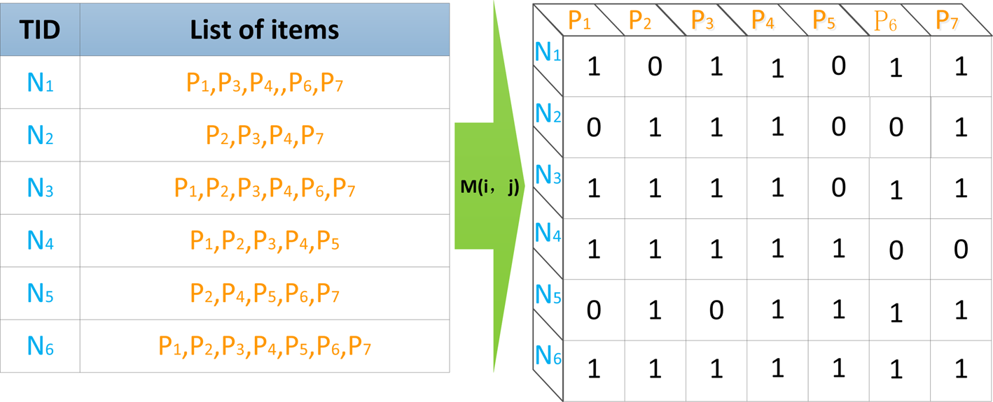
Fig. 5. Data preprocessing.
Determination of initial concentration of pheromone based on BPSO
Setting the initial pheromone concentration is the most critical parameter for determining the performance impact of the ant colony algorithm. To avoid blindness and improve the efficiency of the algorithm, this paper uses the iterative process of the particle swarm algorithm to get a certain set of frequent terms as the initial pheromone concentration of the algorithm. The binary matrix item set after data preprocessing is treated as a particle, and the items represented by the particle must be frequent, with the particle position set to a vector of 0-1.
Each particle in the particle swarm algorithm can remember where it fits best from the initial moment to the current moment. Therefore, by calculating the particle fitness function, the individual extreme x pbest and the global extreme x gbest of the particle can be updated, thus updating the particle position at time t through Eqs (5) and (6).
 $$\eqalign{v^j( {t + 1} ) = & \omega \cdot v^j( t ) + k_1\cdot r_1[ {x_{\,p{\rm best}}^j ( t ) -x^j( t ) } ] \cr & \quad + k_2\cdot r_2[ {x_{g{\rm best}}^j ( t ) -x^j( t ) } ] } $$
 $$x^j( {t + 1} ) = x^j( t ) + v^j( {t + 1} ) $$
 In the equation, v j(t) and x j(t) are the velocities and locations obtained after the first iteration of t for the first example of j. v j(t + 1) and x j(t + 1) are the speed and position of the next moment, respectively;  $x_{p{\rm best}}^j ( t )$ and
  $x_{{\rm gbest}}^j ( t )$ are the individual optimal positions and global optimal positions of particle j at time t, respectively. k 1 and k 2 are learning factors. r 1 and r 2 are random numbers between (0,1); ω is an inertial weight and plays an important role in balancing global and local search capabilities. In order to improve the performance of the algorithm, a linear reduction strategy of inertial weights is used, which enables the algorithm to have a strong search ability at the beginning and get relatively accurate results at the later stage. The adjusted inertial weights are:
 $$\omega = \omega _{{\rm max}}-\displaystyle{{( \omega _{{\rm max}}-\omega _{{\rm min}}) t} \over {T_{{\rm max}}}}$$
In the equation, ω max and ω min are the maximum and minimum values of inertial weights; T max is the maximum number of iterations of the algorithm.
However, the resulting position is not a 0–1 vector, so it needs to be converted using Eq. (8).
 $${\it l}( {\it t}) ^j = \left\{{\matrix{ {1{\rm , \;\ }} & {r_3 < {\rm sig}( {{\it l}{( {\it t} ) }^j} ) } \cr {0{\rm , \;\ }} & {r_3 \ge {\rm sig}( {{\it l}{( {\it t} ) }^j} ) } \cr } } \right.$$
In the equation, r 3 is a random number evenly distributed among (0,1); sig(lt) represents a probability function. In this paper, the |sig(lt)| is used as the probability activation function. The purpose is to ensure that the probability of position change is greater when the absolute value of particle velocity is larger, and the position does not change when the velocity approaches zero, so that it is easier to approach the global optimal particle.
Mining maximum frequent itemsets based on ACO
After removing the initial pheromones of the ant colony algorithm by the particle swarm algorithm, the maximum frequent itemsets in the association rules can be mined by the improved ant colony algorithm for RMS. Similar to the ant colony algorithm's process of finding the optimal path, tabu tables (Tabu) and allowed tables (Allowed) are set to store data items. Initially, ants are randomly placed in different data items as starting points, and data items are added to the set f k where the selected data items are stored to the tabu table. Then, the probability transfer function values of all the remaining optional data items are calculated by Eq. (9) and the next item is selected accordingly.
 $$P_j^k ( t ) = \left\{{\matrix{ {\displaystyle{{\tau_j{( t ) }^\alpha {\rm \eta }_j{( t ) }^\beta } \over {\mathop \sum \nolimits_j \tau_j{( {\rm t} ) }^\alpha {\rm \eta }_j{( t ) }^\beta }}{\rm , \;\ }} \hfill & {\,j\in {\rm allowe}{\rm d}_k} \hfill \cr {0, \;} \hfill & {\,j\in {\rm tab}{\rm u}_k} \hfill \cr } } \right.$$
where τ j(t) is the pheromone concentration at time t;  ${\rm \eta }_j( t )$ is a heuristic function.
Select the data item corresponding to the maximum value of  $P_j^k ( t )$ to add f k to determine if f k is a frequent itemset. If the local pheromone concentration is updated according to Eq. (10) and added to the tabu table, delete it from the allowed table and start the next search.
 $$\tau _{ij}( t ) = ( {1-\varepsilon } ) \cdot \tau _{ij}( t ) + \varepsilon \cdot \Delta \tau _{ij}( t ) $$
 $$\Delta \tau _{ij}( t ) = \mathop \sum \limits_{k = 1}^m \Delta \tau _{ij}( t ) ^k$$
 $$\Delta \tau _{ij}( t ) ^k = \left\{{\matrix{ {Q, \;} \hfill & {{\rm Point\;}i, \;\;j\;{\rm in\;the\;}f_k\;{\rm set\;of\;ant\;}k} \hfill \cr {0, \;} \hfill & {{\rm Other}} \hfill \cr } } \right.$$
If f k is not a frequent itemset after joining, delete it from f k and decide whether to continue the search based on Eq. (13).
 $${\rm stop_{\it k}} = \left\{{\matrix{ {1{\rm , \;\ }} & {\,p > p_0} \cr {0{\rm , \;\ }} & {{\rm Other\;}} \cr } } \right.$$
In the equation, p is the random number on [0,1]. p 0 is a fixed value between [0,1]. If stopk = 1, stop searching. If stopk = 0, the item set is placed in the tabu table and deleted from the allowed table, then the search continues. After all, ants have completed a single traversal, record the maximum frequent itemset that they traversed.
Before the start of the next iteration, according to the positive feedback of the ant colony algorithm, after the ant colony finishes a search, pheromone updates are made on the edges formed by the most frequent item focus points in this iteration. The following are the ways:
 $$\tau _{ij}( {t + 1} ) = ( {1-\rho } ) \cdot \tau _{ij}( t ) + \rho \cdot \Delta \tau _{ij}( t ) $$
 $$\Delta \tau _{ij}( t ) = \left\{{\matrix{ {\displaystyle{Q \over {L_{{\rm best}}}}{\rm , \;\ }} \hfill & {{\rm If}\;i, \;\;j\;{\rm is\;in\;a\;frequent\;itemset}} \hfill \cr {0{\rm , \;\ }} \hfill & {{\rm other}} \hfill \cr } } \right.$$
Rule filtering
Through the above algorithm, we can get a set of rules with high fitness values but often contain similar rules. Therefore, this paper adopts the concept of similarity to filter association rules effectively. If the precursor and successor of one rule contain the precursor and successor of another association rule, there is a similarity between the two rules, and the similarity between the association rule ARi and ARj is:
 $$f_{{\rm sim}}[ {i, \;j} ] = \displaystyle{{S( {{\rm A}{\rm R}_i, \;{\rm A}{\rm R}_j} ) } \over {S( {{\rm A}{\rm R}_i} ) }}$$
In the equation, f sim[i, j] are the random numbers between (0,1). When f sim[i, j] is close to 1, the association rule ARi has a strong similarity with ARj; When f sim[i, j] approaches 0, the association rule ARi has a weak similarity to ARj. If the similarity between two rules is greater than the specified redundancy threshold, that is, if f sim[i, j] ≥ maxfsim is satisfied, then the similarity rule is called the similarity rule, and only the rules with better support in both rules need to be retained.
Algorithm flow
The BPSO-ACO algorithm mainly consists of three parts: one is the preprocessing process of RMS data; the other is mining the largest frequent itemset; the third is generating strong association rules. The entire algorithm flow is as follows.
Step1: Data preprocessing. According to the pattern of association rule mining, the transaction dataset is transformed into binary form to form a two-dimensional matrix data format. Matrix rows represent data records and columns represent transaction attributes.
Step2: Determining the initial pheromone concentration. In order to solve the mining blindness of the ant colony algorithm alone and improve the efficiency of the algorithm, this paper uses a particle swarm algorithm to find a certain number of frequent itemsets to determine the initial pheromone concentration of the ant colony algorithm.
Step3: Population initialization. At the initial moment, each ant is randomly placed in a different data item as the starting point, and the data item is added to the set where the existing data item is saved.
Step4: Extracting the largest frequent itemset. Based on the transfer probability function of all the remaining optional data items, a search procedure is developed to complete traversal of all the populations and record the largest set of frequent items found during this traversal.
Step5: Pheromone update. Before the start of the next iteration search process, the edges composed of points in the optimal frequent itemsets obtained from the last search are updated with pheromones based on the positive feedback of the ant colony algorithm.
Step6: Generating candidate association rules. Repeat step 4, step 5 reaches the maximum number of iterations, outputs the maximum frequent itemset, and obtains a set of corresponding strong association rules.
Step7: After the candidate rules are generated, use the similarity measure to compare the two rules and eliminate the poor rules. Repeat this process to get the final result by pruning the rule set.
Case study
In the process of steel production, the rolled steel cannot be directly used in industrial production because of thermal expansion and errors in rolling equipment, so it needs to be straightened. Straightener is the key equipment for metal shaping in the steel production line. It can straighten metal bars, pipes, and wires. However, in a harsh production environment, it is straightforward to cause various kinds of damage to the equipment. Timely low-cost and effective maintenance of equipment has become a common demand of enterprises. The structural complexity of hot rolling mills determines the diversity of their remanufacturing process demands. This paper takes the RMS of the hot rolling mill as an example, extracts the relationship between service demands and RMS from the historical data of RMS, and provides support for enterprises to obtain effective RMSquickly.
Data collection and description
The schematic diagram of a typical straightener structural component module and its corresponding conventional RMS processes is shown in Figure 6. The encoding scheme proposed in this paper encodes 11 typical hot rolling mill structural parts and 9 remanufacturing processes in historical service data. As shown in Tables 2 and 3, some hot rolling mill remanufacturing transaction records are selected to complete data coding and data mining. Table 2 is the structural part of straightener remanufacturing demands as the lead of the association rules, and Table 3 is the RMS process as the follow-up of the rules. In the table, 1 indicates that the data record contains the transaction attribute, and 0 indicates that it does not.

Fig. 6. Typical straightener structural parts and remanufacturing process.
Table 2. Remanufactured parts of straightener

Table 3. Historical RMS process

Results and discussion
For the above hot rolling mill parts and their historical RMS process data encoding, the association rule mining method based on BPSO-ACO rule mining algorithm is used for experimentation. Associate the remanufacturing parts of a given hot rolling mill with the remanufacturing process data. The mining result is shown in Table 4, which contains the matrix of association rules for all the associated rules. The cells highlighted in bold in the table represent the relationship between the corresponding remanufactured parts and the RMS process.
Table 4. Association rule matrix

The information provided by the above association rule matrix can also be expressed in another form, as shown in Table 5. A total of seven interesting rules have been found that reveal the relationship between hot rolling mill remanufacturing parts and remanufacturing processes. The arrows in the table indicate the matching RMS process methods, support represents the proportion of transactions that contain the rule, and “netconf” represents the proportion of transactions that contain the rule's precursor that also includes the rule's successor. For example, rule 7 indicates that the transactions of alignment process in the work roll remanufacturing process account for 92.3% in the total records, and the transactions of alignment process in the work roll remanufacturing record account for 100%.
Table 5. Association rule extraction of remanufacturing data

The above rules can give full play to their advantages of auxiliary design and guiding significance in practical production and application. On the one hand, after obtaining the service demand issued by customers, the service platform can quickly design the service scheme under the guidance of the corresponding rules and push the RMS provider with service capability to it. Customers can choose the appropriate service provider based on their own cost and quality demands. For example, when a customer provides a RMS demand for the straightener's intermediate roller, the platform invokes relevant rules to assist the designer in providing a service solution quickly. According to the analysis of historical data, the main remanufacturing processes of the intermediate roll are straightening and turning, which are determined by the failure mode of the intermediate roll, and the RMS providers with corresponding service capacity are matched accordingly.
On the other hand, this research also has some guiding significance for the service capability improvement of RMS providers. Under the existing RMS mode, the service provider's passive service mode makes its rich remanufacturing functions not fully developed. As a result, RMS providers can combine existing service functions according to the rules, while producing more and more sophisticated composite services to meet customers’ complex service demands.
The influence of uncertain parameters α,β on mining rules during algorithm execution is verified experimentally so that they can have a positive impact on mining rules. Relatively good combinations of parameters were extracted through repeated experiments, as shown in Table 6. In the subsequent experimental verification process, select the best set of parameters combination α = 2, β = 1 for the experiment.
Table 6. Parameter combination

To measure the response of data mining results to service demands, the experimental results were evaluated using extraction degree (Luna et al., Reference Luna, Ondra and Fardoun2019). Among them, the degree of extraction represents the proportion of all transactions that are supported by rules that meet the set confidence threshold in all historical service data. Define hit ratio as:
 $$R_{{\rm hit}} = \displaystyle{{n_{{\rm hit}}} \over {n_{{\rm total}}}}$$
In the equation, n total represents all remanufacturing history service data with data mining experiments; n hit represents the number of rules that meet the criteria.
Rule mining degree of Apriori algorithm and FP-Growth algorithm used in traditional data mining, ant colony algorithm, and improved algorithm under different levels of support are compared through experiments, as shown in Figure 7. Compared with the traditional data mining algorithm, the improved intelligent algorithm has been improved in the mining effect.

Fig. 7. Rule quality comparison.
The experiment compares the average running time of traditional data mining algorithm and intelligent algorithm at different levels of support, as shown in Figure 8. When the degree of support changes, the efficiency of the traditional algorithm will be greatly affected, but the performance of the intelligent algorithm is more stable. On the basis of the classical ant colony algorithm, BPSO-ACO algorithm optimizes pheromone concentration by particle swarm optimization algorithm and uses the ant colony algorithm to mine the maximum frequent itemset, which improves the operation effect.

Fig. 8. Comparison of operation time.
Conclusion and future work
To solve the problem of extracting effective association rules in RMS scheme matching, we proposed a combined heuristic rule mining method based on BPSO-ACO and established the association rule model of RMS schema matching. Firstly, the mining problem of an association rule is transformed into a discrete particle optimization problem based on decimal encoding. Afterwards, the ant position is updated using particle swarm optimization and ant colony algorithm. By using rule similarity and reducing redundancy rules in the evolution process, a set of effective and optimal association rules is obtained.
In the case study, this method is applied to the RMS scheme design of steel production equipment, and assistant designers can efficiently formulate service schemes to meet the service demands. It can effectively obtain the association rules between the service demand module and the RMS module. At the same time, the weaknesses of the study are also found. Due to the high uncertainty of RMS, complex association rules may have a negative impact on the formulation of service schemes. Therefore, it still needs to rely on the experience and technology of designers for correction. In addition, the method presented in this paper is difficult to combine the advantages of mining results and execution efficiency in the context of scale data, so active data filtering is needed to provide an application basis.
In the future, we will try more ways. Aiming to generate more accurate rules to provide more alternatives for designers, we will study the adaptation of RMS systems deeply. Achieve friendly collaboration between data mining methods and designers and give full play to the advantages of data mining methods.
Acknowledgements
This work was supported in part by the National Natural Science Foundation of China (51805385, 71471143) and the Graduated Science and Technology Innovation Foundation of Wuhan University of Science and Technology (18ZRA061).
Wenbin Zhou was born in Dingxi city, Gansu province in 1994. He received a B.S. degree in Industrial Engineering from the Wuhan University of Science and Technology in 2017. He got the qualification of postgraduate recommendation. Since 2018, he is pursuing a Ph.D. degree in Mechanical Engineering at the Wuhan University of Science and Technology. From 2017 to 2018, he participated in the volunteer teaching program in western China. His research interests include manufacturing systems engineering, networked manufacturing, and remanufacturing services.
Xuhui Xia was born in Hubei, China in 1966. He received his B.S. degree in Mining Machinery from Hubei Polytechnic University in 1988, M.S. degree in Metallurgical Machinery from the Wuhan University of Science and Technology in 1997, and Ph.D. degree in Mechanical Engineering (Industrial Engineering) from Chongqing University in 2003. From 2003 to 2006, he was an Associate Professor with the College of Machinery and Automation, Wuhan University of Science and Technology. Since 2006, he has been a Professor with Department of Industrial Engineering and Manufacturing, Wuhan University of Science and Technology. He is the author of five books, more than 80 articles, and more than 15 inventions. His research interests include manufacturing/remanufacturing systems engineering, reverse supply chain, and related services. Professor Xia’s awards and honors include the Second prize of Hubei science and technology progress award in 2006, the third prize of Hubei Technical Invention award in 2006, the first prize of Hubei science and technology progress award in 2010, and the second prize of Hubei science and technology progress award in 2002.
Zelin Zhang was born in Wuhan, Hubei, China in 1988. He received a B.S. degree in bioengineering and a Ph.D. degree in mineral process engineering from China University of Mining and Technology, Xuzhou, China, in 2009 and 2014, respectively. From 2014 to present, he was an Associate Professor in the Wuhan University of Science and Technology, Wuhan, China. His research interest includes the development of green remanufacturing of mineral processing machinery, Green remanufacturing services, and intelligent mineral processing technology and equipment. Mr. Zhang has won the national scholarship of China, presided over and participated in a number of national scientific research projects, and published more than 30 academic papers.
Lei Wang was born in Hubei, China in 1987. She received her B.S. degree in Electrical Engineering and Automation from Hubei Polytechnic University in 2008, M.S. degree in Mechanical Manufacturing and Automation from the Wuhan University of Science and Technology in 2010, and Ph.D. degree in Industrial Engineering from the Wuhan University of Science and Technology in 2017. From 2010 to 2017, she was an engineer with the Engineering Training Centre of Wuhan University of Science and Technology, mainly engaged in the design and development of Manufacturing Execution & information System, and electronic circuit. Since 2017, she has been a lecturer with Department of Industrial Engineering and Manufacturing, Wuhan University of Science and Technology. She is the author of three books, more than 30 articles, and more than six inventions. Her research interests include manufacturing systems engineering, reverse supply chain management, remanufacturing, and related services. Dr. Wang was a recipient of the second prize of Hubei science and technology progress award: Green manufacturing technology and application of typical mechanical parts in 2014.


