Nomenclature
-
 $\textbf{A}$
-
state matrix
- A–PC
-
aircraft–pilot coupling
-
$\textbf{B}$
-
input matrix
-
$\textbf{C}$
-
output matrix
-
$\textbf{c}$
-
input vector
-
$\textbf{D}$
-
feedforward matrix
-
${e(s)}$
-
error signal between the desired value and the actual aircraft
-
$g$
-
gravitational acceleration
-
$\mathrm{I}_{y}$
-
moment of inertia about the y-axis
-
$\mathrm{K}_{p}$
-
gain
- LQR
-
linear quadratic regulator
-
$m$
-
mass of the aircraft
- PIO
-
pilot-induced oscillation
-
$q$
-
pitch rate
- ROVER
-
real-time oscillation verifier
-
$\mathrm{T}_{L}$
-
general lead time constant of human pilot modelling function
-
$\mathrm{T}_{I}$
-
general lag time constant of human pilot modelling function
-
$u(s)$
-
pilot control signal
-
$\Delta u$
-
longitudinal velocity variation
-
$w$
-
vertical velocity
-
$\textbf{x}$
-
state vector
-
$\mathrm{X}_{\cdot }$
,
$\mathrm{I}_{\cdot }$
,
$\mathrm{M}_{\cdot }$
-
stability and control longitudinal derivatives
-
$\textbf{y}$
-
linearised flight dynamics
-
$\mathrm{Y}_{c}$
(s)
-
transfer function for the aircraft behaviour
-
$\mathrm{Y}_{p}$
(s)
-
transfer function for human pilot action


Greek symbol
-
$\delta_{e}$
-
elevator angle
-
$\Delta\theta$
-
pitch angle variation
-
$\zeta$
-
damping coefficient
-
$\theta_{0}$
-
initial pitch angle
-
$\tau$
,
$\tau_{e}$
-
time delay constant
-
$\omega_{c}$
-
crossover frequency
-
$\omega_{n}$
-
natural frequency


1.0 Introduction
Pilot-Induced Oscillation (PIO), also known as Aircraft–Pilot Coupling (A–PC), can be defined as “sustained or uncontrollable oscillations resulting from efforts of the pilot to control the aircraft” [1]. In other words, it is a coupling between the dynamics of a system (in this case, an aircraft) and the action of the pilot trying to control the oscillations but, instead of attenuating them, the controller aggravates the problem [Reference Wang, Santone and Cao2]. Although an old issue that has been studied since the 1960s [Reference Ashkenas3], new PIO incidents, and even accidents, still occur in modern aircraft. The constant increase in performance and the introduction of new technologies foster research to revisit the topic from time to time [Reference Toader and Ursu4]. The detection and suppression of PIO situations have been addressed by scientific researchers since the 1960s, and their results have shown that this phenomenon cannot be detected prior to its occurrence, although some algorithms propose real-time identification of the event, including the Real-time Oscillation Verifier (ROVER), which observes four parameters and their threshold values in order to characterise a PIO.
With the advancement of computational tools and the development of more reliable aircraft models, computational simulations have become a great ally in the analysis of PIO occurrences, as they are much cheaper and safer than carrying out in-flight test campaigns, which expose the aircraft to potential damage and endanger the test crew. Given that both the aircraft and the human pilot participate in a PIO, models of the vehicle dynamics and the human being are necessary for a representative simulation.
Several advances have been made towards high-fidelity physics-based aircraft models, which are now widely available, for example, through sets of control and stability derivatives in a state-space formulation. Computational pilot models have also benefited from recent major developments, especially the so-called functional models. However, to date, it is still unclear how these pilot models can be used to simulate PIO conditions.
To fill this gap, this study analysed the feasibility of using three different computational pilot models (Tustin [Reference Tustin5], Crossover and Precision [Reference McRuer and Krendel6]) to simulate pitch PIO conditions. Tests were performed in MATLAB® for three aircraft models with different levels of propensity to PIO, as well as for two pilot gain conditions. A purely longitudinal synthetic task was used to induce potential PIOs, and a tuned real-time PIO detection algorithm (ROVER) was utilised to detect the condition.
The current paper is structured into the following main sections: Section 2 presents the modelling addressed for the PIO study, detailing the aircraft and pilot models, the synthetic task and the PIO detection algorithm, including some considerations about the flight commands; Section 3 details the data collection and estimation parameters required by the pilot functional models to perform the PIO computational simulations; Section 4 presents and discusses the findings. Finally, Section 5 provides concluding remarks. This work is part of a broader research project towards the study of PIO events [Reference Moura, Bidinotto and Belo7,Reference Moura8].
2.0 Modelling
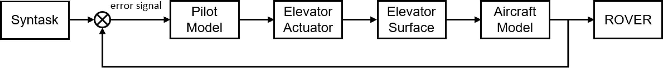
In this manuscript, potential PIO conditions were assessed using the control arrangement shown in Fig. 1. It essentially consisted of a generic task to be performed (Syntask), a human pilot model, an aircraft model and a PIO detection algorithm (ROVER). Figure 1 also includes the elevator actuator and the elevator surface, representing the whole pitch flight control system. These are sources of delays and may affect the behaviour of the system in PIO [Reference Wang, Santone and Cao2,Reference Ashkenas3,Reference Moura, Bidinotto and Belo7–Reference Moura, Alegre, Bidinotto and Belo9], but in the current study, such delays were disregarded because they could compromise the information sought by the research.

Figure 1. Diagram of the system used.
The study focused on pitch PIO, thus only the longitudinal motion of the aircraft was considered and the pitch angle was chosen as the parameter to be controlled. That said, the error signal e(s) shown in Fig. 1 accounted for the difference between the longitudinal reference attitude (the Syntask) and the actual pitch angle of the aircraft. Based on this signal, the pilot model actuated on the aircraft dynamics by deflecting the elevator (being the only possible input signal).
The behaviour of the human pilot is either represented by three different pilot models in the form of transfer functions proposed in the literature or by a real human, whereas the aircraft is modelled by the closed-loop configuration with a Linear Quadratic Regulator (LQR) controller. It is noteworthy that the actuators of the aircraft control surfaces have some limitations, thus their rate and position saturation were also modelled and incorporated into the vehicle dynamics model. The rate limit of the actuators was chosen to be
 $40^{\circ}$
/s, and the position of the control surfaces was limited to deflect
$40^{\circ}$
/s, and the position of the control surfaces was limited to deflect
 $30^{\circ}$
for each side. Finally, the ROVER algorithm is utilised to identify in real time the occurrence of PIO [Reference Moura, Alegre, Bidinotto and Belo9].
$30^{\circ}$
for each side. Finally, the ROVER algorithm is utilised to identify in real time the occurrence of PIO [Reference Moura, Alegre, Bidinotto and Belo9].
The main blocks of the control arrangement of Fig. 1 are detailed in the remainder of this section.
2.1 Syntask
Syntask is a synthetic task consisting of a profile of attitudes (in our case, the pitch angle) to be carried out by either human or computational pilots. In this study, the Syntask was displayed on the artificial horizon by means of a movable red line (Fig. 2a). The line moved in accordance with the profile indicated in Fig. 2b. All simulations with the computational pilot models were performed using the same Syntask profile (Fig. 2b).
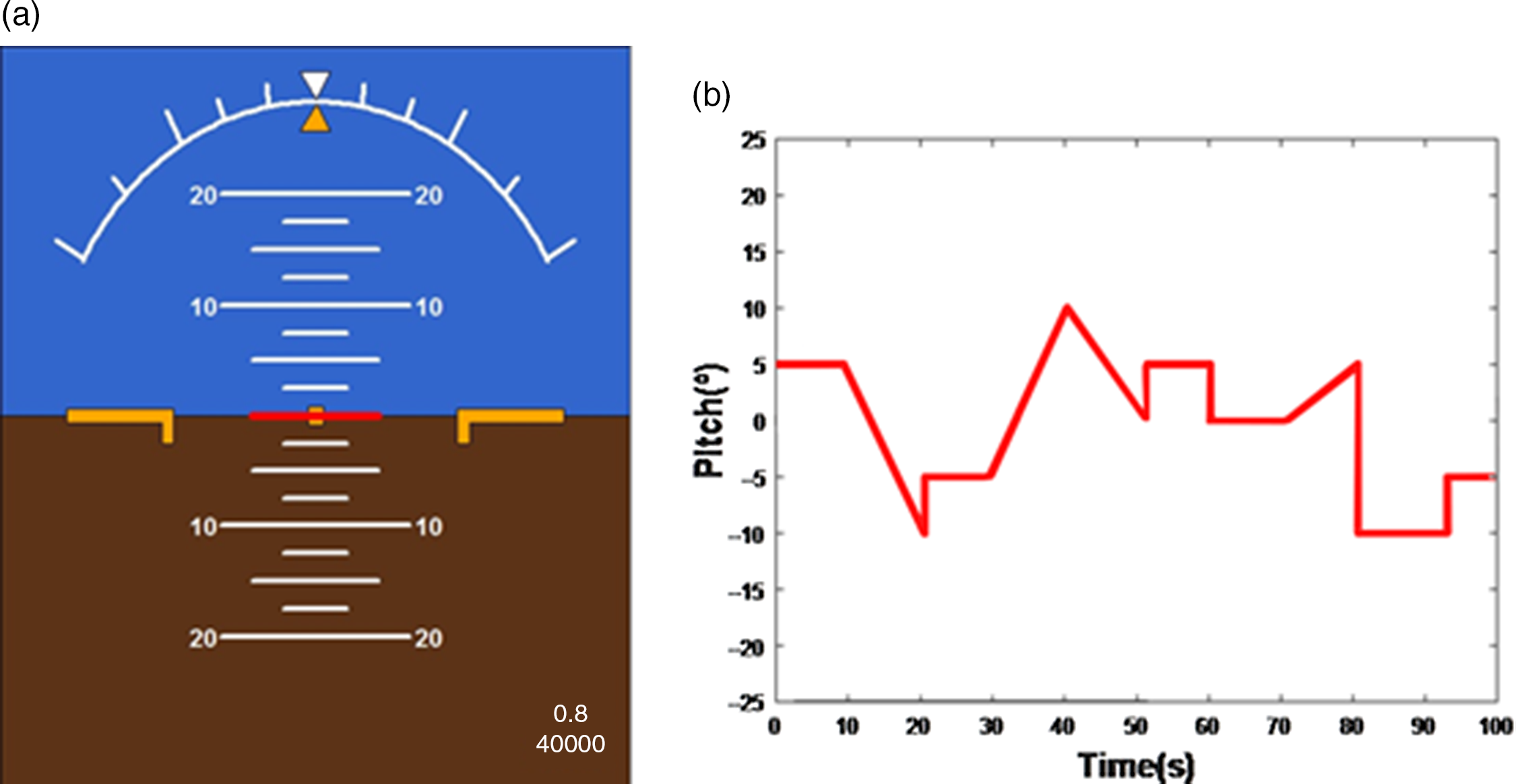
Figure 2. Synthetic task system [Reference Moura8].
2.2 Aircraft model
A state-space approach according to Etkin and Reid (10) is selected to model the dynamics of the vehicle, in this case, a Boeing 747-100 in a cruise condition equivalent to an altitude of 40,000ft and Mach 0.8. Equation (1) describes the system via the state-space optics, in which the state vector
 $\textbf{x}$
represents the longitudinal velocity variation (
$\textbf{x}$
represents the longitudinal velocity variation (
 $\Delta$
u), vertical velocity (w), pitch rate (q) and pitch angle variation (
$\Delta$
u), vertical velocity (w), pitch rate (q) and pitch angle variation (
 $\Delta\theta$
). It can thus be seen that only the longitudinal behaviour is considered, as the research focuses on pitch-axis PIO. For the same reason, the input vector of Equation (1), that is,
$\Delta\theta$
). It can thus be seen that only the longitudinal behaviour is considered, as the research focuses on pitch-axis PIO. For the same reason, the input vector of Equation (1), that is,
 $\textbf{c}$
, stands for the elevator angle (
$\textbf{c}$
, stands for the elevator angle (
 $\delta_{e}$
), while the output vector
$\delta_{e}$
), while the output vector
 $\textbf{y}$
in the present research coincides with the state vector. Therefore, the output matrix
$\textbf{y}$
in the present research coincides with the state vector. Therefore, the output matrix
 $\textbf{C}$
is a
$\textbf{C}$
is a
 $4\times4$
identity matrix, whilst the feedthrough matrix
$4\times4$
identity matrix, whilst the feedthrough matrix
 $\textbf{D}$
is a
$\textbf{D}$
is a
 $4\times1$
null matrix. The throttle is considered to be constant.
$4\times1$
null matrix. The throttle is considered to be constant.
 \begin{eqnarray}\dot{\textbf{x}} = \textbf{Ax} + \textbf{Bc}\end{eqnarray}
 \begin{eqnarray}\textbf{y} = \textbf{Cx} + \textbf{Dc},\nonumber\end{eqnarray}
which are presented as the Equations (2) and (3) when written in full mode
 \begin{eqnarray}\left\{\begin{array}{c} \Delta \dot{u}\\ \dot{w}\\ \dot{q} \\ \Delta \dot{\theta} \end{array}\right\} =\left(\begin{array}{cccc} \frac{X_{u}}{m} & \frac{X_{w}}{m} & 0 & -g\cos(\theta_{0}) \\ \frac{Z_{u}}{m - Z\dot{_{w}}} & \frac{Z_{w}}{m - Z\dot{_{w}}} & \frac{Z_{q} - m u_{0}}{m - Z\dot{_{w}}} & \frac{- m g \sin(\theta_{0})}{m - Z\dot{_{w}}} \\ \frac{1}{I_{y}}\left[M_{u} + \frac{M\dot{_{w}} Z_{u}}{\left(m - Z\dot{_{w}}\right)}\right] & \frac{1}{I_{y}}\left[M_{w} + \frac{M\dot{_{w}} Z_{u}}{\left(m - Z\dot{_{w}}\right)}\right] & \frac{1}{I_{y}}\left[M_{q} + \frac{M\dot{_{w}} \left(Z_{q} + m u_{0}\right)}{\left(m - Z\dot{_{w}}\right)}\right] & -\frac{M\dot{_{w}} m g \sin(\theta_{0})}{I_{y}\left(m - Z\dot{_{w}}\right)} \\ 0 & 0 & 1 & 0 \end{array}\right)\left\{\begin{array}{c} \Delta u\\ w\\ q \\ \Delta\theta \end{array}\right\}\nonumber \\+\left(\begin{array}{c} \frac{X_{\delta_{e}}}{m}\\ \frac{X_{\delta_{e}}}{m - Z\dot{_{w}}}\\ \frac{M_{\delta_{e}}}{I_{y}}+\frac{M\dot{_{w}} Z_{\delta_{e}}}{I_{y}\left(m - Z\dot{_{w}}\right)} \\ 0 \end{array}\right)\delta_{e},\end{eqnarray}
 \begin{equation}\textbf{y} =\left(\begin{array}{c@{\quad}c@{\quad}c@{\quad}c} 1 &0 &0 &0 \\ \\[-7pt] 0 &1 &0 &0 \\ \\[-7pt] 0 &0 &1 &0 \\ \\[-7pt] 0 &0 &0 &1 \end{array}\right)\left\{\begin{array}{c} \Delta u\\ \\[-7pt] w\\ \\[-7pt] q \\ \\[-7pt] \Delta\theta \end{array}\right\}+\left(\begin{array}{c} 0 \\ \\[-7pt] 0 \\ \\[-7pt] 0 \\ \\[-7pt] 0 \end{array}\right)\delta_{e}.\end{equation}
According to the assumption of decoupling between the longitudinal and lateral directional motions, Equations (2) and (3) apply to the motion relative to the axis in the wingspan direction (y). In these equations, m is the mass of the aircraft, g is the gravitational acceleration and
 $I_{y}$
is the moment of inertia about the y-axis; the other terms are the longitudinal stability derivatives of the aircraft, detailed in Table 1.
$I_{y}$
is the moment of inertia about the y-axis; the other terms are the longitudinal stability derivatives of the aircraft, detailed in Table 1.
Table 1. The stability and control derivative of the models [Reference Moura, Alegre, Bidinotto and Belo9,Reference Etkin and Reid10]
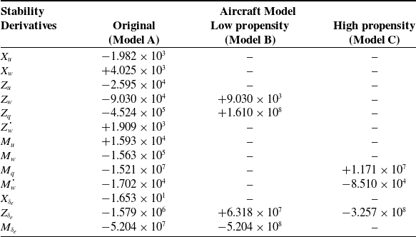
A thorough investigation is conducted in the sense that three different sets of stability derivatives are analysed, as presented in Table 1. The first, model A, represents the original parameters for the mentioned flight condition [Reference Etkin and Reid10], whilst models B and C [Reference Moura, Alegre, Bidinotto and Belo9], correspond to modified variables, with B being a model with lower propensity to PIO occurrence and C having a higher propensity. In Table 1, the derivatives omitted for models B and C mean that the original value was maintained.
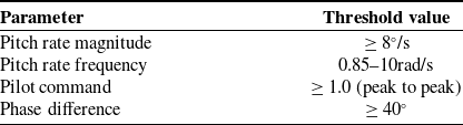
2.3 ROVER algorithm
The ROVER algorithm seeks to detect PIO in real time by observing four parameters: (i) pitch rate magnitude, (ii) pitch rate frequency, (iii) pilot input amplitude and (iv) phase difference [Reference Mitchell, Arencibia and Munoz11]. When all these parameters simultaneously reach pre-established threshold values, the algorithm flags that the system is in PIO.
These parameter values were chosen according to Liu [Reference Liu12] and have been previously tested in other works from the same authors [Reference Moura, Bidinotto and Belo7–Reference Moura, Alegre, Bidinotto and Belo9]. In these trials, some human pilots were subjected to similar conditions and their subjective opinion corroborated the use of the values presented in Table 2.
Table 2. ROVER parameters [Reference Mitchell, Arencibia and Munoz11,Reference Liu12]

2.4 Pilot models
Three mathematical pilot models were used in this study. Although differing slightly, they all seek to mathematically represent the control action of a human pilot by means of a transfer function
 $Y_{p}(s)$
modelling the pilot control signal u(s) for the error signal e(s). The three models together with their transfer functions are described below.
$Y_{p}(s)$
modelling the pilot control signal u(s) for the error signal e(s). The three models together with their transfer functions are described below.
2.4.1 Tustin model
Tustin [Reference Tustin5] proposed the transfer function presented herein as Equation (4) to model the human pilot control action. In this model, the pilot’s control behaviour, level of experience and neuromuscular limitations are taken into account. These parameters are respectively represented in Equation (4) by the gain
 $K_p$
, the time constant of anticipation
$K_p$
, the time constant of anticipation
 $T_{L}$
and the time delay constant
$T_{L}$
and the time delay constant
 $\tau$
.
$\tau$
.
 \begin{equation}Y_{p} = \frac{u(s)}{e(s)} = \frac{K_{p}(1+T_{L}s)e^{-\tau s}}{s}.\end{equation}
2.4.2 Crossover model
According to McRuer [Reference McRuer and Krendel6], human pilots adapt their control actions depending on how they perceive the dynamic condition of the controlled vehicle, thus that author proposed an open-loop transfer function for the pilot–vehicle system as presented in Equation (5).
 \begin{equation}Y_{p}Y_{c} = \frac{\omega_{c}e^{-\tau_{e} s}}{s}.\end{equation}
In this model,
 $Y_{c}(s)$
and
$Y_{c}(s)$
and
 $Y_{p}(s)$
represent the individual transfer functions of the vehicle and pilot, respectively, whereas
$Y_{p}(s)$
represent the individual transfer functions of the vehicle and pilot, respectively, whereas
 $\omega_{c}$
is the so-called crossover frequency and
$\omega_{c}$
is the so-called crossover frequency and
 $\tau_{e}$
is a total time delay constant modelling the time elapsed between the instant when a change in the system behaviour is identified by the human body and the moment the aircraft changes its attitude as a consequence of an action performed by the crew member.
$\tau_{e}$
is a total time delay constant modelling the time elapsed between the instant when a change in the system behaviour is identified by the human body and the moment the aircraft changes its attitude as a consequence of an action performed by the crew member.
Based on the mentioned pilot–vehicle system model, McRuer further explored the pilot behaviour and introduced a transfer function solely describing the human being as expressed in Equation (6). The presence of a time delay constant (
 $T_{I}$
) suggests the adoption of this model when the response of a controlled plant is dominated by a second-order transfer function, which serves well the aircraft modes of phugoid, short-period and Dutch roll. Additionally,
$T_{I}$
) suggests the adoption of this model when the response of a controlled plant is dominated by a second-order transfer function, which serves well the aircraft modes of phugoid, short-period and Dutch roll. Additionally,
 $K_{p}$
stands for the gain of the pilot, and
$K_{p}$
stands for the gain of the pilot, and
 $\tau$
serves as their response time delay.
$\tau$
serves as their response time delay.
 \begin{equation}Y_{p} = \frac{u(s)}{e(s)} = \frac{K_{p}e^{-\tau s}}{T_{I}s+1}.\end{equation}
2.4.3 Precision model
Likewise developed by McRuer [Reference McRuer and Krendel6], the precision model expands the crossover model to take into account the human neuromuscular actuation system and an anticipation component for the pilot’s control action. The general form of its describing function is defined in Equation (7). In addition to the pilot gain
 $K_p$
, time delay
$K_p$
, time delay
 $\tau$
and general lag time constant
$\tau$
and general lag time constant
 $T_I$
also considered in the crossover model, Equation (7) introduces the lead time constant
$T_I$
also considered in the crossover model, Equation (7) introduces the lead time constant
 $T_L$
towards the lead-lag pilot control actuation, as well as the term in parentheses to account for the neuromuscular system. Regarding the latter,
$T_L$
towards the lead-lag pilot control actuation, as well as the term in parentheses to account for the neuromuscular system. Regarding the latter,
 $\omega_{n}$
and
$\omega_{n}$
and
 $\zeta$
respectively represent the natural frequency and damping ratio of the pilot’s neuromuscular system.
$\zeta$
respectively represent the natural frequency and damping ratio of the pilot’s neuromuscular system.
 \begin{equation}Y_{p} = K_{p}e^{-\tau s}\frac{T_{L}s + 1}{T_{I}s + 1}\left(\frac{1}{\frac{s^2}{\omega_{n}^2}\frac{2\zeta}{\omega_{n}}s+1}\right).\end{equation}
To utilise the models presented above, the parameters of each transfer function were obtained from experimental data gathered from human pilot trials. Thus, a model estimation methodology was applied, as detailed in the next section.
3.0 Model estimation
Human pilot trials are conducted to estimate the variables required by the pilot models. For this purpose, three volunteer pilots, identified as pilot 1, pilot 2 and pilot 3, were asked to fly the Boeing 747 model in the above-detailed cruise situation (Section 2.2). In these tests, the system shown in Fig. 1 still applies, except for the pilot model which is substituted by the human pilot, and the ROVER system, which in this case is not utilised.
The trials consist of the generation of a synthetic task in the form of a step from 0
 $^\circ$
to 10
$^\circ$
to 10
 $^\circ$
(or 10
$^\circ$
(or 10
 $^\circ$
to 0
$^\circ$
to 0
 $^\circ$
).Footnote 1 with respect to the artificial horizon (Fig. 2a). The pilots are then required to capture the angle using a commercial joystick with a 40Hz acquisition rate.
$^\circ$
).Footnote 1 with respect to the artificial horizon (Fig. 2a). The pilots are then required to capture the angle using a commercial joystick with a 40Hz acquisition rate.
In addition, for the characterisation of a PIO condition, the pilot must apply the command in an aggressive manner [Reference Mitchell and Klyde13], simulating an emergency situation. This way, both conditions are simulated: slow application (called normal gain condition) and fast application (called high gain condition). Hereinafter, these modes are also named susceptibility conditions.
Figures 3 and 4 present the results obtained for the three test pilots performing the task just described. In both cases, the Pitch Task curve (red) represents the synthetic task that the pilot should follow, while the Pilot Command contour (black) shows the angle applied on the joystick by the test pilot, and finally, the curve labelled Model Angle (blue) is the attitude of the aircraft model following the command application. Figure 3 applies to the normal gain condition, whilst Fig. 4 refers to the high gain situation.
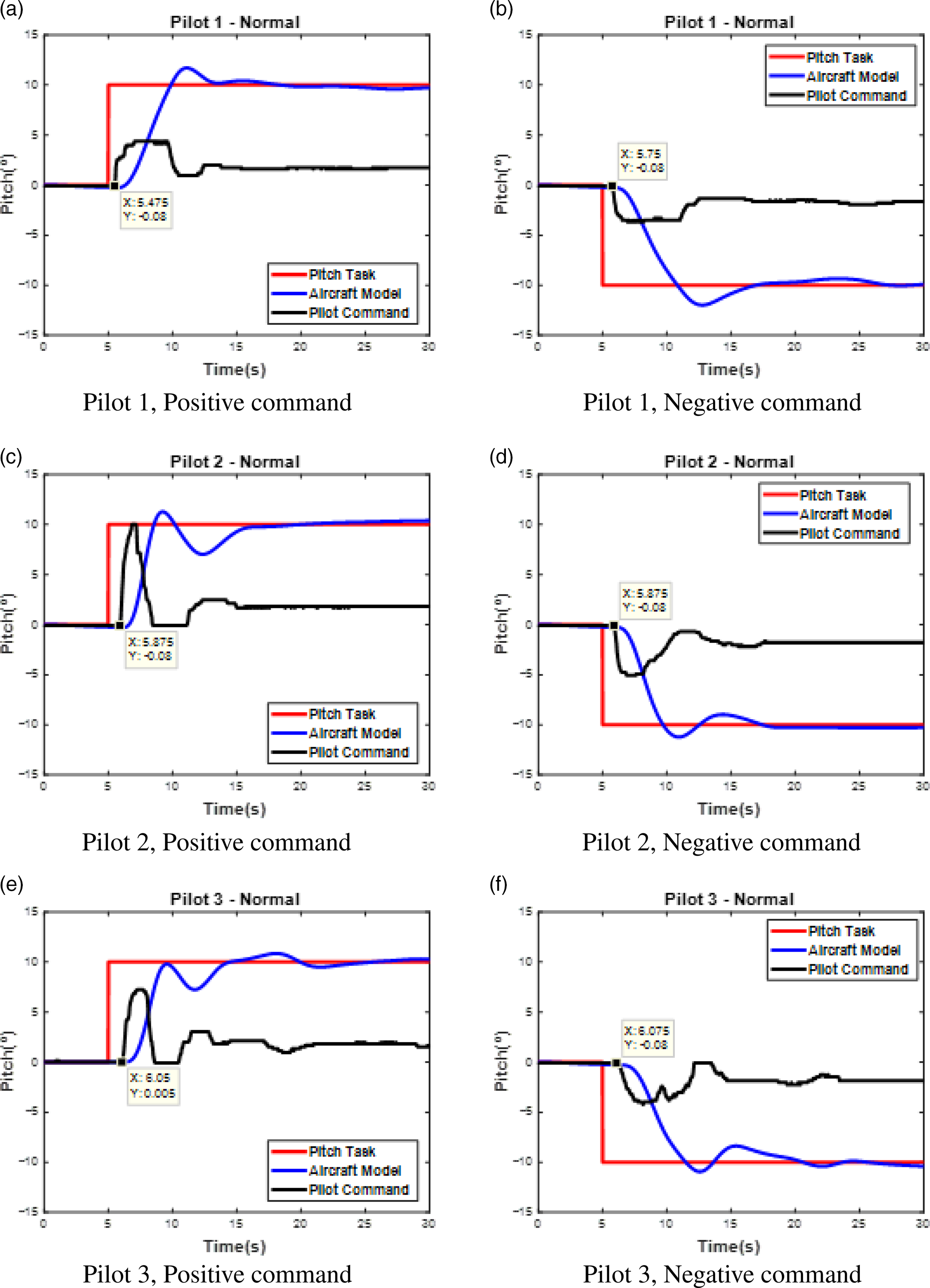
Figure 3. Pilot model estimation: Syntask, aircraft pitch angle and pilot input for the normal gain condition.
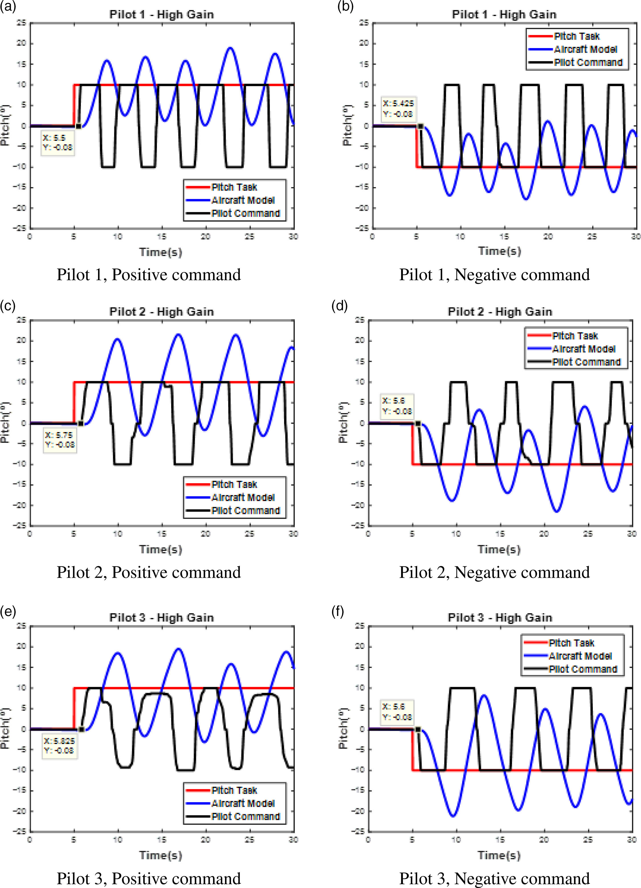
Figure 4. Pilot model estimation: Syntask, aircraft pitch angle and pilot input for the high gain condition.
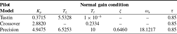
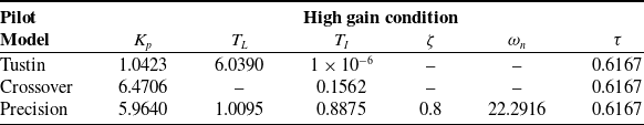
From the data presented in Figs. 3 and 4, the parameters of interest for the three pilot models were extracted, for both the normal and high gain conditions, as presented in Table 3 and 4, respectively. To accomplish this task, the MATLAB® system identification toolbox was used, although due to limitations of the mentioned toolbox in identifying the real value of the pilot time delay, the pole of Tustin’s model, originally at the origin, was dislocated, resulting in the transfer function described in Equation (8)
 \begin{equation}Y_{p} = \frac{K_{p}(T_{L}s + 1)}{(T_{I}s + 1)}e^{-\tau s}.\end{equation}
Table 3. Pilot model estimation: parameters for the normal gain condition

Table 4. Pilot model estimation: parameters for the high gain condition

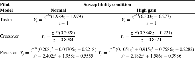
Finally, Table 5 provides the transfer functions for the three pilot models according to the gain condition. Entries in Table 5 are in the Z-domain (discrete-time), i.e.,
 \begin{equation}Y_{p} = \frac{u(z)}{e(z)}\end{equation}
Table 5. Pilot model estimation: Z-domain transfer functions

4.0 Results
To investigate the PIO phenomenon, a series of mathematical simulations were conducted with the Boeing 747-100 in cruise condition. Referring to Fig. 1, Syntask corresponds to a given imposed task to be performed, whereas pilot model stands for the derived pilot functional models (Section 3, Table 5) in both normal and high gain conditions; furthermore, the aircraft model is substituted by the three vehicle models detailed in Table 1. Finally, the ROVER algorithm, as discussed in Sect. 2.3, is utilised to indicate the occurrence (or not) of PIO.
The results are presented in Figs 5, 6 and 7. All of them present the control responses for the three pilot models (Tustin, Crossover and Precision) and susceptibility conditions (normal and high gain), although Fig. 5 refers to the original aircraft model (model A), whilst Figs. 6 and 7 correspond to the aircraft dataset with low (model B) and high (model C) propensity for PIO, respectively.
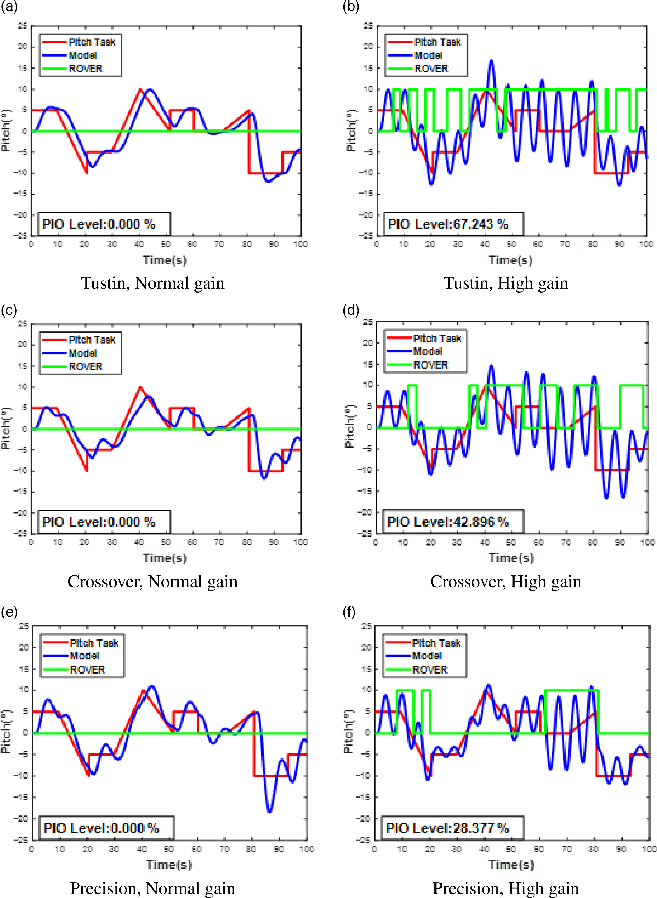
Figure 5. Syntask, Aircraft pitch angle and ROVER for all pilot models and gain conditions: original aircraft model (A).
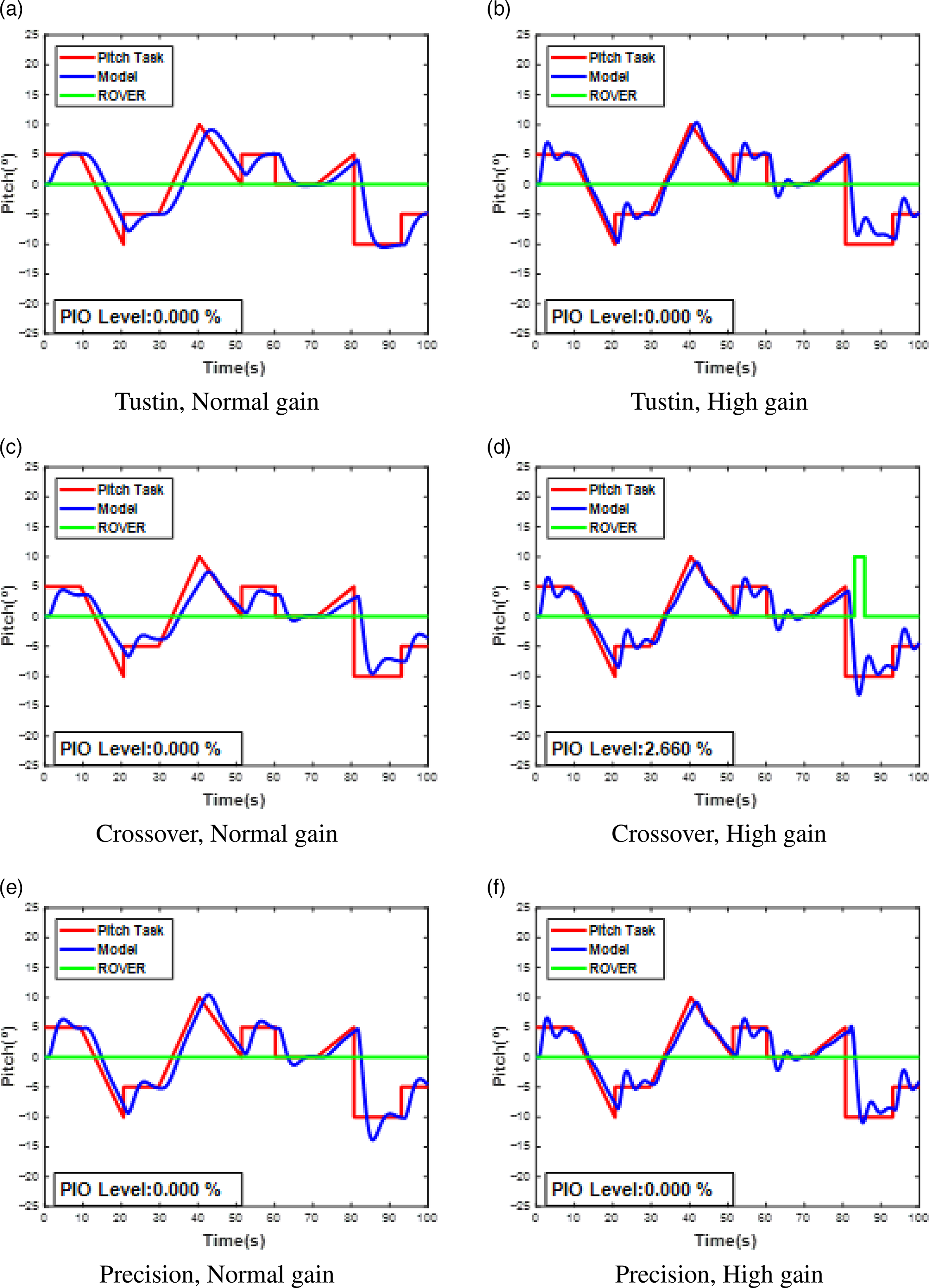
Figure 6. Syntask, Aircraft pitch angle and ROVER for all pilot models and gain conditions: low propensity model (B).
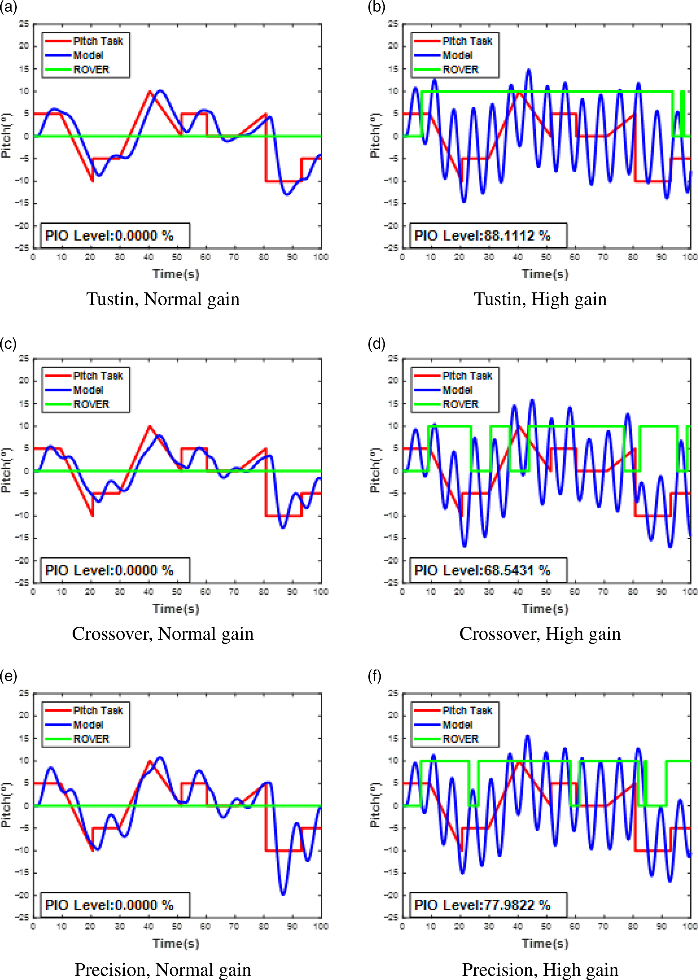
Figure 7. Syntask, Aircraft pitch angle and ROVER for all pilot models and gain conditions: high propensity model (B).
Additionally, in each figure, the Pitch Task (red) curve represents the synthetic task proposed to the virtual pilot, the Model contour (blue) shows the response of the pilot-controlled aircraft model and the ROVER curve (green) indicates the PIO condition based on the detection subroutine. In more detail, when the ROVER curve is zero, the pilot–aircraft set lies outside the PIO condition, while on the other hand, when it assumes non-zero values (in this case chosen to be 10 in order to be better visualised in the figures), it means that the set is coupled, i.e., in a PIO condition.
Moreover, Fig. 5, 6 and 7 also present the variable PIO Level, that is, the percentage of time for which the ROVER curve is in 10 (non-null). As the subroutine serves for the detection of a PIO situation, it is possible to infer that, the higher the PIO Level, the more susceptible to the phenomenon the pilot–aircraft system will be.
5.0 Conclusions
In the light of the collected results, it is possible to state that the proposed system architecture, as presented in Fig. 1, is effective for simulating the high gain condition, with both human and virtual pilots. Since the three pilot models were successfully applied in the simulations, it can be concluded that the methodology for estimating their transfer function parameters is adequate; moreover, as the ROVER subroutine identified the coupling between the aircraft and pilot, it can be concluded that the algorithm is valid for detecting PIO.
Based on theoretical literature, the high gain manoeuvring condition was expected to show a greater tendency to PIO when compared with the low-gain applications, which is indeed confirmed by the PIO level observations in Fig. 5, 6 and 7. Additionally, independently of the pilot model adopted, the aircraft models with low (B) and high (C) propensity for PIO proved to be in accordance with theoretical expectations, as the PIO level of these plants is considerably lower and higher, respectively, in comparison with the original aircraft dynamics. These observations are valid for the high gain command application condition.
For the low propensity aircraft model (B), only the Crossover pilot activated the ROVER algorithm (Fig. 6d). In comparison with the response obtained for the other virtual pilots, the mentioned model presents the greatest residual oscillation about the pitch task, which triggers the ROVER, confirming the sensitivity of the detection algorithm.
However, in this sense, for the high propensity aircraft model (C), the virtual pilot proposed by Tustin showed greater susceptibility to sustaining oscillations with the aircraft, being a more conservative option when studying pilot–aircraft coupling behaviour without the application of any type of control. On the other hand, for the original aircraft model (A), the virtual Crossover pilot model had a greater tendency to PIO when compared with the Precision model, whereas for the high propensity (C) model, the opposite is observed, with the Precision virtual pilot having a slightly greater tendency than the Crossover pilot representation.
In future research addressing PIO, it is recommended to identify the threshold values of the stability derivatives for cases with greater propensity for this phenomenon. Also, a project is already underway with the aim of deeper characterisation of the loss of control in flight phenomenon, which also includes the PIO problem based on a parametric analysis of pilot inputs and aircraft behaviour in both longitudinal and lateral axes.
In the near future, the authors aim to develop a tool that could detect and suppress the PIO condition in real time, to avoid future accidents caused by this phenomenon.
Acknowledgements
This work was supported by FAPESP (grant no. 2016/16808-5) and CNPq scholarship.