NOMENCLATURE
- BTT
bank-to-turn
- C yα, C yδz
aerodynamic lift coefficients related with angle of attack and elevator
- C zβ, C zδy
lateral force coefficients related with sideslip angle and rudder
- d α1, d α2
lift uncertainty coefficients related with angle of attack and elevator
- d β1, d β2
lateral force uncertainty coefficients related with sideslip angle and rudder
- d x
roll moment uncertainty coefficient related with aileron
- d y1, d y2
yaw moment uncertainty coefficients related with sideslip angle and rudder
- d z1, d z2
pitch moment uncertainty coefficients related with attack angle and elevator
- DOF
degree of freedom
- J x, J y, J z
moments of inertial in terms of x, y, z axis of body coordinate system
- L
characteristic length
- m
missile mass
- m xδx
roll moment coefficient related with aileron
- m yβ, m y δy
yaw moment coefficients related with sideslip angle and rudder
- m zα, m z δz
pitch moment coefficients related with attack angle and elevator
- M x, M y, M z
aerodynamic moments with respect to roll, yaw and pitch
- P
engine thrust
- q
dynamic pressure calculated by q = 0.5ρV 2
- s
missile reference area characteristic length.
- STT
skid-to-turn
- TSMC
terminal sliding mode control
- V
flight velocity
- Y
aerodynamic lift
- Z
lateral force
- α, β, γ
angle of attack, sideslip and roll
- w x, w y, w z
angular velocities in terms of x, y, z axis of body coordinate system
- δ x, δ y, δ z
deflections of aileron, rudder, and elevator
- ρ
air density
- θ
pitch angle
1.0 INTRODUCTION
With increasing demands of weapon tactical performance under complex battlefield environment, the bank-to-turn (BTT) missile has drawn significant attention because of its long range, high accuracy and superior manoeuvrability compared with conventional skid-to-turn (STT) missiles.
General BTT missiles adopt a non-axial symmetric configuration. The maximum lift surface is oriented rapidly to the desired direction by a roll movement whereas the attitude angle of sideslip in yaw channel remains fixed, constituting the coordinate manoeuvring movement. This characteristic inevitably induces heavy nonlinear crossing couplings and interactions between different channels, which typically contributes to the intrinsic nonlinear dynamics of the BTT missile. Meanwhile, the influence caused by aerodynamic parameters is more severe than that of the STT missile, indicating that aerodynamic perturbations remain to be taken into consideration during the controller design process. Additionally, for a missile flight system, a well-behaved controller not only tracks the command swiftly, but exhibits certain robustness against disturbances and uncertainties existed throughout the fickle flight regime. From the point of overall design, it is also preferable to evaluate the control performances as much as possible once preliminary controller deign is accomplished.
In the past decades, a number of strategies have been proposed. Refs. (Reference McGehee and Emmert1) and (Reference Arrow and Williams2) design the autopilot in pitch and yaw channel independently without considering nonlinear items at the beginning. By utilizing an adaptive anti-disturbance control algorithm and adding coordinate-loops respectively, the influences of nonlinear couplings have been compensated. Ref. (Reference Crater and Shamma3) transformed the missile dynamics to a linear parameter varing form, and then applied a gain scheduling method. Based on the linearisation method with the assumption of small perturbation theory and fixed parameter hypothesis, classical control method, like the PI control( Reference Lin and Yueh4 ), root locus and frequency control( Reference Kovach, Stevens and Arrow5 ), and pole placement method( Reference Sun and Qi6 ) are applied on the linear dynamic model. However, these methods fail to interact with couplings and uncertainties directly, and the overall system may be constrained when the interactions between different channels are severe. To improve this, more advanced techniques towards nonlinear control and robustness are introduced. Refs. (Reference Lin and Wang7) and (Reference Kang, Jin Kim, Lee, Jun and Tahk8) combined H∞ control algorithm with linear parameter varying (LPV) synthesis and neural networks repectively. Ref. (Reference Choi, Lee and Choi9) utilised the dynamic inversion method to design the control input, together with the extended-mean technique dealing with system uncertainties. To improve system performance when encountering severe. To improve system performance when encountering severe disturbances, Ref. (Reference Li and Jun10) employed the the disturbance observer technique to compensate for the unknown couplings and external disturbances. In Refs. (Reference Zheng, Liu, Yang and Du11) and (Reference Xu, Yu, Yuan and Gu12), the fusion of adaptive sliding-mode control and fuzzy logic was considered, enabling the controller to demonstrate multiple advantages of both control algorithms.
Among abundant controller design approaches, the sliding-mode control (SMC) has obtained extensive attention for its remarkable robustness. The characteristics of fast response, interference immunity, and insensitivity to the bounded disturbances make it suitable for the BTT controller design( Reference Pisano and Elio13 , Reference Kumar, Rao and Ghose14 ). Typical SMC method involves two items, namely the sliding manifold and reaching law. The former generally comprises tracking errors in relation to control objectives while the latter accounts for motivating system states “on sliding mode”. Linear sliding manifolds, together with corresponding linear reaching laws, provide asymptotic stability of control variables in sliding movement, which means system states converge to the equilibrium point exponentially at infinite time( Reference Zhou, Mu and Xu15 ). Then the algorithm is improved as terminal sliding mode control (TSMC) with finite time convergence property. Refs. (Reference Wang, Li and Fei16) and (Reference Chen, Wu and Cui17) introduced functions to determine the reaching law, with which control variables reach the desired values within finite time. Refs. (Reference Yu and Long18) and (Reference Khoo, Xie, Zhao and Man19) have succedded in accomplishing the finite-time consensus of a second-order multi-agent system and higher-order multi-agent system, respectively. In Ref. (Reference Mobayen20), a new form of switching surface is introduced to derive a novel fast TSMC approach, where the reaching phase is eliminated to improve the global robustness of the system. To avoid singularity problems induced by higher order nonlinear functions, Refs. (Reference Wang and Wang21) and (Reference Kumar, Rao and Ghose22) finished similar deductions of nonsingular TSMC algorithm, ensuring the feasibility of controller implementation. In Ref. (Reference Zhao and Hua23), a new continuous nonlinear distributed consensus tracking protocol is constructed via a nonsingular terminal sliding mode (TSM) scheme.
However, in the above finite time convergence-related works, detailed estimations of settling time are not addressed. Only theoretical results are provided in the citation of lemmas. From the given mathematical version of theoretical settling time, the convergence rate can be estimated on the condition that prior knowledge of system initial states are available. Diverse initial conditions correspond to various settling time, indicating that the maximum value depends on the largest initial error related with the Lyapunov function. It is significant that the settling time can be predicted when initial conditions are unknown, both for preliminary design and engineering application. Thus in contrast with existing finite-time controllers, the upper bound of the settling time can be estimated in the sense of fixed-time convergence concept( Reference Polyakov24 ), in which the bounded convergence time is independent of system initial conditions. With the newly constructed sliding mainfold, Ref. (Reference Zuo25) achieved a nonsingular fixed time consensus tracking for second-order multi-agent networks. Carried the idea farther, it expanded the fixed-time terminal sliding mode control methods for a class of second-order nonlinear systems( Reference Zuo26 ). In Ref. (Reference Jiang, Hu and Friswell27), a controller in the sense of fixed-time convergence concept has been constructed for rigid spacecraft, in which the attitude angles converged to the equilibrium points within the defined fixed time even with actuator saturation and faults. Based on distributed control strategy with observers, Ref. (Reference Fu and Wang28) proposed two novel controllers to deal with the fixed-time coordinated tracking problem for second order multi-agent system.
Further, to interact with disturbances, variable structure items which comprise discontinuous schemes like the signum function are normally employed in the SMC control methodologies mentioned above. The discontinuous signum function induces the well-known chattering phenomenon as the switching gain need to be defined larger than the bound of uncertainties, which degrades system performance and prohibits implementation of the controller. Some works substituted the discontinuous item with saturation function or sigmoid function( Reference Wang, Zong, Dong and Tian29 ), whereas control effectiveness is sacrificed to a certain degree. Refs. (Reference Li and Jun10) and (Reference Awad and Wang30) utilised the the disturbance observer to estimate the uncertainties. Despite the fact that control burden can be reduced with ESO’s output incorporated into control input as a feedforward scheme, the discontinuous item is inevitably unavoidable, and the system suffers from the chattering phenomenon inevitably. Meanwhile, the bandwidth of the disturbance observer has to be selected wide enough to cover the frequency of the nonlinear coupling terms, which is a tradeoff between robustness and control performance. To alleviate chattering effectively, an integrated roll-pitch-yaw autopilot based on global TSMC control was synthesised in Ref. (Reference Wang, Zong, Dong and Tian29) with a partial state nonlinear observer without using the signum function.
Motivated by previous work, a smooth adaptive sliding-mode-based controller for BTT missiles has been designed in our research with fixed time convergence in the presence of nonlinear couplings and aerodynamic uncertainties. Adaptive estimations with some mathematical results are incorporated to derive the control algorithm. Unlike existing BTT missile controllers, the designed approach motivates missile attitude variables, namely the angle of attack, sideslip, and roll, converge to the equilibrium points before the predefined bounded settling time in the presence of nonlinear couplings and aerodynamic uncertainties. The control input is inherently continuous without introducing any discrete items, like the signum function. The upper bound of setting time is simply a function of designed parameters, indicating that prior information about the convergence rate can be obtained at a preliminary design period without acquiring system initial conditions. Within the known uniform bounded convergence time, BTT controller can track the desired command at any given initial states, which is of significant value for both overall missile design and performance evaluation. The smooth input of the designed BTT controller avoids the problem of singularity and chattering, which not only ensures better performance of missile control system, but simultaneously provides considerable availability for practical implementation. Comprehensive simulations are carried out to demonstrate the superior performance of the designed BTT controller. The fixed time convergent characteristics are fully reflected in the cases of separate controller gains and initial states. Meanwhile the smooth inputs exhibit nice continuity in spite of nonlinear couplings and aerodynamic uncertainties.
The rest of this paper is organised as follows. Nonlinear BTT missile dynamics is presented in the forthcoming section. Decomposed into loop structures, Section 3 introduces some preliminaries and elaborates the smooth adaptive sliding mode-based controller design process, in which the fixed time convergence theory is synthesised. In Section 4, detailed stability analysis are provided via Lyapunov theory. Various simulations are performed in Section 5 with specific analysis to validate the effectiveness of the designed approach, and finally, conclusions are given in Section 6.
2.0 BTT MISSILE DYNAMIC MODEL FORMULATION
Conventional control problem of BTT missiles embodies the tracking of the commanded angle of attack, sideslip and roll. The nonlinear attitude dynamic model is formulated in the presence of gravity, crossing couplings and aerodynamic uncertainties, which is suitable for the generic tail-controlled BTT missiles in non axial-symmetric winged configuration.
In controller design procedures, it is quite usual to assume that flight altitude is fixed with a constant velocity, and the aerodynamic uncertainties, as well as their derivatives, are all bounded. The airframe is considered to be governed by rigid body mechanics, which indicates that aero-elasticity, static parameter variations, like mass, and moment of inertial are neglected through the entire flight. Besides, precise measurement of attitude angles and angular velocities can be acquired with advanced onboard sensors.
Then, the complete 6-DOF dynamic model of BTT missile is depicted as
 $$\left\{ {\matrix{
{\dot \alpha = {\omega _z} - {\omega _x}\tan \beta \cos \alpha + {\omega _y}\tan \beta \sin \alpha - {{(P\sin \alpha + Y)} \over {mV\cos \beta }}} \hfill \cr
{\qquad + {g \over {V\cos \beta }}(\sin \vartheta \sin \alpha + \cos \vartheta \cos \gamma \cos \alpha )} \hfill \cr
{\dot \beta = {\omega _x}\sin \alpha + {\omega _y}\cos \alpha + {{Z - P\cos \alpha \sin \beta } \over {mV}}} \hfill \cr
{\qquad + {g \over V}(\sin \vartheta \cos \alpha \sin \beta - \cos \vartheta \cos \gamma \sin \alpha \sin \beta + \cos \vartheta \sin \gamma \cos \beta )} \hfill \cr
{\dot \gamma = {\omega _x} - \tan \vartheta ({\omega _y}\cos \gamma - {\omega _z}\sin \gamma )} \hfill \cr
{{{\dot \omega }_x} = {{{J_y} - {J_z}} \over {{J_x}}}{\omega _z}{\omega _y} + {{{M_x}} \over {{J_x}}}} \hfill \cr
{{{\dot \omega }_y} = {{{J_z} - {J_x}} \over {{J_y}}}{\omega _x}{\omega _z} + {{{M_y}} \over {{J_y}}}} \hfill \cr
{{{\dot \omega }_z} = {{{J_x} - {J_y}} \over {{J_z}}}{\omega _x}{\omega _y} + {{{M_z}} \over {{J_z}}}} \hfill \cr
} } \right.$$
$$\left\{ {\matrix{
{\dot \alpha = {\omega _z} - {\omega _x}\tan \beta \cos \alpha + {\omega _y}\tan \beta \sin \alpha - {{(P\sin \alpha + Y)} \over {mV\cos \beta }}} \hfill \cr
{\qquad + {g \over {V\cos \beta }}(\sin \vartheta \sin \alpha + \cos \vartheta \cos \gamma \cos \alpha )} \hfill \cr
{\dot \beta = {\omega _x}\sin \alpha + {\omega _y}\cos \alpha + {{Z - P\cos \alpha \sin \beta } \over {mV}}} \hfill \cr
{\qquad + {g \over V}(\sin \vartheta \cos \alpha \sin \beta - \cos \vartheta \cos \gamma \sin \alpha \sin \beta + \cos \vartheta \sin \gamma \cos \beta )} \hfill \cr
{\dot \gamma = {\omega _x} - \tan \vartheta ({\omega _y}\cos \gamma - {\omega _z}\sin \gamma )} \hfill \cr
{{{\dot \omega }_x} = {{{J_y} - {J_z}} \over {{J_x}}}{\omega _z}{\omega _y} + {{{M_x}} \over {{J_x}}}} \hfill \cr
{{{\dot \omega }_y} = {{{J_z} - {J_x}} \over {{J_y}}}{\omega _x}{\omega _z} + {{{M_y}} \over {{J_y}}}} \hfill \cr
{{{\dot \omega }_z} = {{{J_x} - {J_y}} \over {{J_z}}}{\omega _x}{\omega _y} + {{{M_z}} \over {{J_z}}}} \hfill \cr
} } \right.$$
with
 $$\left\{ \begin{array}{l}Y = \left[ {(1 + {d_{\alpha 1}})C_y^\alpha \alpha + (1 + {d_{\alpha 2}})C_y^{{\delta_z}}{\delta_z}} \right]qs\\ Z = \left[ {(1 + {d_{\beta 1}})C_z^\beta \beta + (1 + {d_{\beta 2}})C_z^{\delta y}{\delta_y}} \right]qs\\ {M_x} = (1 + {d_x})m_x^{{\delta_x}}{\delta_x}qsL\\ {M_y} = \left[ {(1 + {d_{y1}})m_y^\beta \beta qsL + (1 + {d_{y2}})m_y^{{\delta_y}}{\delta_y}} \right]qsL\\ {M_z} = \left[ {(1 + {d_{z1}})m_z^\alpha \alpha + (1 + {d_{z2}})m_z^{{\delta_z}}{\delta_z}} \right]qsL\end{array} \right.$$
where C y*, C z*, m x*, m y* and m z* are coefficients of corresponding aerodynamic force and moment-related with attitude angles and actuator deflections. As assumed at the beginning, all of the coefficients representing aerodynamic perturbations, namely, d α1, d α2, d β1, d β2, d x, d y1, d y2, d z1, d z2 are bounded. δ x, δ y, δ z are control input variables.
From Eq. (1), it is apparent that BTT missile dynamics comprises kinematical coupling, aero dynamical coupling, inertial coupling and control couplings, which significantly contribute to the nonlinearity of the control problem. Rearrange Eqs. (1) and (2) to form the following nonlinear system:
 $$\left\{ \begin{array}{l}{{{\dot{\boldsymbol{x}}}}_1} = {{\boldsymbol{f}}_1} + {{\boldsymbol{g}}_1}{{\boldsymbol{x}}_2} + {{\boldsymbol{d}}_1}\\ {{{\dot{\boldsymbol{x}}}}_2} = {{\boldsymbol{f}}_2} + {{\boldsymbol{g}}_2}{\boldsymbol{u}} + {{\boldsymbol{d}}_2}\end{array} \right.$$
 $${{\bf{x}}_{\bf{1}}} = \left[ {\matrix{
\alpha \cr
\beta \cr
\gamma \cr
} } \right],\;{{\bf{x}}_{\bf{2}}} = \left[ {\matrix{
{{\omega _x}} \cr
{{\omega _y}} \cr
{{\omega _z}} \cr
} } \right],\;{\bf{u}} = \left[ {\matrix{
{{c_1}{\delta _x}} \cr
{{b_4}{\delta _y}} \cr
{{a_4}{\delta _z}} \cr
} } \right]$$
$${{\bf{x}}_{\bf{1}}} = \left[ {\matrix{
\alpha \cr
\beta \cr
\gamma \cr
} } \right],\;{{\bf{x}}_{\bf{2}}} = \left[ {\matrix{
{{\omega _x}} \cr
{{\omega _y}} \cr
{{\omega _z}} \cr
} } \right],\;{\bf{u}} = \left[ {\matrix{
{{c_1}{\delta _x}} \cr
{{b_4}{\delta _y}} \cr
{{a_4}{\delta _z}} \cr
} } \right]$$
 $${{\bf{f}}_1} = \;\left[ {\matrix{
{\matrix{
{ - {{{a_1}\alpha + {d_1}\sin \alpha } \over {\cos \beta }} + {g \over {V\cos \beta }}(\sin \vartheta \sin \alpha + } \hfill \cr
{\qquad \qquad \cos \vartheta \cos \gamma \cos \alpha )} \hfill \cr
} } \cr
{\matrix{
{{b_1}\beta - {d_1}\cos \alpha \sin \beta + {g \over V}(\sin \vartheta \cos \alpha \sin \beta + } \hfill \cr
{\cos \vartheta \sin \gamma \cos \beta - \cos \vartheta \cos \gamma \sin \alpha \sin \beta )} \hfill \cr
{\quad \qquad \qquad \qquad \qquad 0} \hfill \cr
} } \cr
} } \right],\;{{\bf{f}}_2} = \left[ {\matrix{
{{{{J_y} - {J_z}} \over {{J_x}}}{\omega _z}{\omega _y}} \cr
{{{{J_z} - {J_x}} \over {{J_y}}}{\omega _x}{\omega _z} + {b_3}\beta } \cr
{{{{J_x} - {J_y}} \over {{J_z}}}{\omega _x}{\omega _y} + {a_3}\alpha } \cr
} } \right]$$
$${{\bf{f}}_1} = \;\left[ {\matrix{
{\matrix{
{ - {{{a_1}\alpha + {d_1}\sin \alpha } \over {\cos \beta }} + {g \over {V\cos \beta }}(\sin \vartheta \sin \alpha + } \hfill \cr
{\qquad \qquad \cos \vartheta \cos \gamma \cos \alpha )} \hfill \cr
} } \cr
{\matrix{
{{b_1}\beta - {d_1}\cos \alpha \sin \beta + {g \over V}(\sin \vartheta \cos \alpha \sin \beta + } \hfill \cr
{\cos \vartheta \sin \gamma \cos \beta - \cos \vartheta \cos \gamma \sin \alpha \sin \beta )} \hfill \cr
{\quad \qquad \qquad \qquad \qquad 0} \hfill \cr
} } \cr
} } \right],\;{{\bf{f}}_2} = \left[ {\matrix{
{{{{J_y} - {J_z}} \over {{J_x}}}{\omega _z}{\omega _y}} \cr
{{{{J_z} - {J_x}} \over {{J_y}}}{\omega _x}{\omega _z} + {b_3}\beta } \cr
{{{{J_x} - {J_y}} \over {{J_z}}}{\omega _x}{\omega _y} + {a_3}\alpha } \cr
} } \right]$$
 $${{\bf{g}}_1} = \left[ {\matrix{
{ - \tan \beta \cos \alpha } & {\tan \beta \sin \alpha } & 1 \cr
{\sin \alpha } & {\cos \alpha } & 0 \cr
{1} & { - \tan \vartheta \cos \gamma } & {\tan \vartheta \sin \gamma } \cr
} } \right],\;{{\bf{g}}_2} = \left[ {\matrix{
{{c_1}} & 0 & 0 \cr
{0} & {{b_4}} & 0 \cr
{0} & 0 & {{a_4}} \cr
} } \right]$$
$${{\bf{g}}_1} = \left[ {\matrix{
{ - \tan \beta \cos \alpha } & {\tan \beta \sin \alpha } & 1 \cr
{\sin \alpha } & {\cos \alpha } & 0 \cr
{1} & { - \tan \vartheta \cos \gamma } & {\tan \vartheta \sin \gamma } \cr
} } \right],\;{{\bf{g}}_2} = \left[ {\matrix{
{{c_1}} & 0 & 0 \cr
{0} & {{b_4}} & 0 \cr
{0} & 0 & {{a_4}} \cr
} } \right]$$
where
 $${a_1} = {{{C_y}^\alpha qs} \over {mV}},\;{a_2} = {{{C_y}^{{\delta _z}}qs} \over {mV}},\;{a_3} = {{{m_z}^\alpha qsL} \over {{J_z}}},{a_4} = {{{m_z}^{{\delta _z}}qsL} \over {{J_z}}}\\{b_1} = {{{C_z}^\beta qs} \over {mV}},\;{b_2} = {{{C_z}^{{\delta _y}}qs} \over {mV}},\;{b_3} = {{{m_y}^\beta qsL} \over {{J_z}}},{b_4} = {{{m_y}^{{\delta _y}}qsL} \over {{J_z}}}\\{c_1} = {{{m_x}^{{\delta _x}}qsL} \over {{J_x}}},{d_1} = {P \over {mV}}$$
and d 1 = [d 11, d 12, d 13]T, d 2 = [d 21, d 22, d 23]T are the bounded uncertainties concerning aerodynamic-related parameters. Define that |d 1i| ≤ σ1i, |d 2i| ≤ σ2i, i = 1, 2, 3 and σ1i, σ2i are all positive constants.
System (3) well represents the complex nonlinear behaviour of BTT missiles steering by actuator deflections. It involves gravitational effect, aerodynamic uncertainties, and highly cross-couplings between different channels. With measurable state variables x 1 and x 2, items like f 1, f 2, g 1, and g 2 can be calculated. The developed nominal dynamic model is suitable to design a nonlinear controller based on robust nonlinear stabilising and tracking control algorithm.
3.0 BTT CONTROLLER DESIGN
In this section, the concept of fixed time stability is introduced first, together with some primary mathematical results. Afterwards, a smooth adaptive sliding-mode-based BTT controller has been designed with fixed time convergence characteristic. The influence of uncertainties is alleviated without the commonly used discontinuous items (like the sign function), and therefore avoid the well-known chattering problems in conventional SMC method.
3.1 Preliminary and design objective
The concept of fixed-time stability can be interpreted as the extension of finite-time stability.
Consider the nonlinear system(Reference Wang, Li and Fei16)
 $${\dot{\bf{x}}} = {\bf{f}}({\bf{x}},t),{\bf{f}}({\bf{0}},t) = {\bf{0}},{\bf{x}} \in {{\bf{R}}^n}$$
where f: U 0 × R →R n is continuous on U 0 × R, and U 0 is an open set of the origin.
The origin is a finite-time stable equilibrium if it is Lyapunov stable and for any given initial time t 0 and initial state x(t 0) = x 0∈U ⊂ U 0, there exists a settling time T ≥ 0, which depends on x 0, such that for every solution of system (5), x(t) = φ(t: t 0, x 0) ∈U /{0}, satisfies
 $$\left\{ {\matrix{
{\mathop {\lim }\limits_{t \to T({x_0})} {\rm{\varphi }}(t:{t_0},{{\bf{x}}_0}) = {\bf{0}},t \in [{t_0},T({x_0})]} \hfill \cr
{{\rm{\varphi }}(t:{t_0},{{\bf{x}}_0}) = {\bf{0}},t > T({x_0})} \hfill \cr
} } \right.$$
$$\left\{ {\matrix{
{\mathop {\lim }\limits_{t \to T({x_0})} {\rm{\varphi }}(t:{t_0},{{\bf{x}}_0}) = {\bf{0}},t \in [{t_0},T({x_0})]} \hfill \cr
{{\rm{\varphi }}(t:{t_0},{{\bf{x}}_0}) = {\bf{0}},t > T({x_0})} \hfill \cr
} } \right.$$
Moreover, if the origin is finite-time stable with U = R n, then the origin is a global finite-time-stable equilibrium. Following lemma provides sufficient condition for the finite convergence-control design( Reference Zhou, Sun and Teo31 ).
Lemma 1: Consider the differential equation of system (4). Suppose there exists a continuous positive-definite function V(x, t):
 $${\hat{\textbf{U}}}$$
→R, where
$${\hat{\textbf{U}}}$$
→R, where
 $${\hat{\textbf{U}}}$$
is a neighborhood of the origin, such that there are real number c > 0 and 0 < a < 1 satisfying
$${\hat{\textbf{U}}}$$
is a neighborhood of the origin, such that there are real number c > 0 and 0 < a < 1 satisfying
 $${\dot{V}}$$
(x, t)+cV α(x, t) ≤ 0 on
$${\dot{V}}$$
(x, t)+cV α(x, t) ≤ 0 on
 $${\hat{\textbf{U}}}$$
. Then the zero solution of system (5) is finite-time stable. The settling time is given by
$${\hat{\textbf{U}}}$$
. Then the zero solution of system (5) is finite-time stable. The settling time is given by
 $$T({{\bf{x}}_0}) \le \frac{{{V^{1 - \alpha }}({{\bf{x}}_0})}}{{c(1 - \alpha )}}$$
In addition, if
 $${\hat{\textbf{U}}}$$
= R
n, and V is radially unbounded, then the origin is globally finite-time stable.
$${\hat{\textbf{U}}}$$
= R
n, and V is radially unbounded, then the origin is globally finite-time stable.
Obviously, the finite convergence time derived from lemma 1 depends on system initial condition. Different initial states correspond to various settling time, which indicates no uniform bound of convergence time can be obtained in advance without the knowledge of maximum V(x 0). If prior information of system initial states is not available, pre-evaluations of controller performance would be restricted to some extent. From the point of preliminary overall design and engineering application, it is preferable that system performance metrics — for example, the bound of settling time — can be estimated beforehand regardless of initial system states. Moreover, for those with strict positive dwelling time, such as hybrid system control, it is necessary to stabilise the controlled system exactly before the next switching occurs( Reference Cruz-Zavala, Moreno and Fridman32 ). Thus moving further on, the concept of fixed-time convergence is put forward.
Consider system (4), the origin is said to be a “fixed-time stable” equilibrium point if it is globally finite-time stable and the settling time function T(x
0) is bounded; that is, there exists T max > 0 such that T(x
0) < T max,
 $$\forall $$
x
0∈R
n.The following lemma presents helpful result for the design of controller with fixed-time convergence(
Reference Kumar, Rao and Ghose22
).
$$\forall $$
x
0∈R
n.The following lemma presents helpful result for the design of controller with fixed-time convergence(
Reference Kumar, Rao and Ghose22
).
Lemma 2: Consider a scalar system
 $$\dot y = - \alpha {y^{\frac{m}{n}}} - \beta {y^{\frac{p}{q}}},y(0) = {y_0}$$
where α > 0, β > 0. m, n, p and q are positive odd integers satisfying m > n, p < q. Then the origin of system (7) is fixed-time stable and the settling time
 $$T$$
is bounded by
$$T$$
is bounded by
 $$T < {T_{\max }}{\rm{ = }}\frac{1}{\alpha }\frac{n}{{m - n}} + \frac{1}{\beta }\frac{q}{{q - p}}$$
As denoted in Eq. (8), the upper bound of settling time is independent of system initial condition and basically determined by designed parameters, namely, m, n, p, q, α, β. Therefore, prior knowledge of “fixed” settling time can be obtained at the beginning with appropriate selection of parameters on the basis of system performance metrics.
Before conducting the BTT controller design, two fundamental equations are supplemented as follows.
 $$\frac{{{{(ab)}^2}}}{{4\mu }} + \mu \ge ab$$
 $$\zeta {c^2} + \frac{{{d^2}}}{{4\zeta }} \ge cd$$
Equations (9) and (10) are mathematically correct and are helpful to prove the stability of the designed controller in the subsequent section.
Design objective: In this paper, a robust smooth adaptive sliding mode controller is proposed with fixed time convergence property for BTT missiles under the condition of nonlinear couplings and aerodynamic uncertainties, with which system states converge to the commanded value within predefined bound of settling time at any initial conditions, and the designed control input is essentially smooth without introducing any discontinuous items.
3.2 BTT smooth adaptive fixed time convergent sliding mode controller
This section derived a robust smooth sliding-mode-based controller with fixed-time convergence for system (3). In the light of time scale separation principal, cascade control structure is employed and therefore (3) is decomposed into outer loop and inner loop architectures. The former accounts for generating proper angular rate command to trace the attitude angle signals, while the latter for operating on the tail deflections to track the reference angular rate command obtained from forward loop.
A. Outer loop
Suppose the desired command is x d and x d = [α d, β d, γ d]T. The objective of outer loop control is to design the angular rate defined as a virtual control input ( x 1c) to make x 1 converge to x d within a fixed bounded time. Rewrite the first equation of system (3) here
 $${{\dot{\boldsymbol{x}}}_1} = {{\boldsymbol{f}}_1} + {{\boldsymbol{g}}_1}{{\boldsymbol{x}}_{1c}} + {{\boldsymbol{d}}_1}$$
Define a sliding manifold as
 $${{\boldsymbol{s}}_1} = {\left[ {{s_{11}},{s_{12}},{s_{13}}} \right]^T} = {{\boldsymbol{x}}_1} - {{\boldsymbol{x}}_d}$$
Taking the derivative of S 1 with respect to time yields
 $${{\dot{\boldsymbol{s}}}_1} = {{\boldsymbol{f}}_1} + {\boldsymbol{g}}{{\boldsymbol{x}}_{1c}} + {{\boldsymbol{d}}_1} - {{\dot{\boldsymbol{x}}}_d}$$
A notation has been employed here to represent the multiplication between scalar and vector
 $$\kappa {{\boldsymbol{\theta}}^r} = {\left[ {\kappa {\theta_1}^r,{\kern 1pt} {\kern 1pt} \kappa {\theta_2}^r, \cdots \kappa {\theta_n}^r} \right]^T}$$
where κ, r are scalar constants and
 $$\boldsymbol{\vartheta}$$
= [ϑ 1, ϑ 2,… ϑ n]T is a R
n vector.
$$\boldsymbol{\vartheta}$$
= [ϑ 1, ϑ 2,… ϑ n]T is a R
n vector.
To achieve the fixed-time convergence, the reaching law is designed in the form
 $${{\dot{\boldsymbol{s}}}_1} = - {\beta_{11}}{{\boldsymbol{s}}_1}^{\frac{{{m_1}}}{{{n_1}}}} - {\beta_{21}}{{\boldsymbol{s}}_1}^{\frac{{{p_1}}}{{{q_1}}}} - {\beta_{31}}{{\boldsymbol{s}}_1} - \frac{{{{{{\hat{\boldsymbol{\chi}}}}}_1}{{\boldsymbol{s}}_1}}}{{4{\mu_1}}} + {{\boldsymbol{d}}_{\rm{1}}}$$
where β 1, β 2, ε1 and µ 1 are non-negative. m 1, n 1, p 1 and q 1 are positive odd constants satisfying m 1 > n 1, p 1 < q 1. The vector fields take the form as indicated in Ref. [Reference Kumar, Rao and Ghose14].
 $${{\hat{\boldsymbol{\chi}}}_1} = diag[{\hat{\chi}_{11}},{\hat{\chi}_{12}},{\hat{\chi}_{13}}]$$
is the estimation of χ
1 = diag[σ 112, σ 122, σ 132] and is determined by the updating law
$${{\hat{\boldsymbol{\chi}}}_1} = diag[{\hat{\chi}_{11}},{\hat{\chi}_{12}},{\hat{\chi}_{13}}]$$
is the estimation of χ
1 = diag[σ 112, σ 122, σ 132] and is determined by the updating law
 $${\dot{\hat{\chi}}_{1i}} = - {\beta_{41}}{\hat{\chi}_{1i}} + \frac{{s_{1i}^2}}{{4{\mu_1}}},{\kern 1pt} {\kern 1pt} {\kern 1pt} i = 1,2,3.$$
where β 41 > 0.
Substitute Eq. (15) into Eq. (13), the virtual control signal of outer loop can be obtained as
 $${{\boldsymbol{x}}_{1c}} = {[{x_{1c1}},{x_{1c2}},{x_{1c3}}]^T} = {{\boldsymbol{g}}_1}^{ - 1}( - {{\bf{f}}_1} - {\beta_{11}}{{\boldsymbol{s}}_1}^{\frac{{{m_1}}}{{{n_1}}}} - {\beta_{21}}{{\boldsymbol{s}}_1}^{\frac{{{p_1}}}{{{q_1}}}} - {\beta_{31}}{{\boldsymbol{s}}_1} - \frac{{{{{\hat{\boldsymbol{\chi}}}}_1}{{\boldsymbol{s}}_1}}}{{4{\mu_1}}} + {\dot x_d})$$
Next, with the obtained virtual control input x 1c from Eq. (17), the control input of angular rate loop can be obtained under same baseline.
B. Inner loop
Similar procedures are implemented in inner loop design. The objective is to deduce the actual control input such that tracking error between the virtual control signal and the actual angular rates converges to the origin within the fixed bounded time. Rewrite the second equation of system (3)
 $${{\dot{\boldsymbol{x}}}_2} = {{\boldsymbol{f}}_2} + {{\boldsymbol{g}}_2}{\boldsymbol{u}} + {{\boldsymbol{d}}_2}$$
Another sliding manifold is defined as
 $${{\boldsymbol{s}}_2} = {\left[ {{s_{21}},{s_{22}},{s_{23}}} \right]^T} = {{\boldsymbol{x}}_2} - {{\boldsymbol{x}}_{1c}}$$
Differentiating S 2 yields
 $$\begin{array}{l}{{{\dot{\boldsymbol{s}}}}_2} = {{\boldsymbol{f}}_2} + {\boldsymbol{u}} + {{\boldsymbol{d}}_2} - {{{\dot{\boldsymbol{x}}}}_{1c}}\\ \quad = {{\boldsymbol{f}}_2} + {\boldsymbol{u}} + {{\boldsymbol{d}}_2}^*\end{array}$$
where
 $${{\boldsymbol{d}}_2}^* = {[{d_{21}}^*,{d_{22}}^*,{d_{23}}^*]^T} = {{\boldsymbol{d}}_2} - {{\dot{\boldsymbol{x}}}_{1c}}$$
. Considering the real situation of the BTT missile control system, ||
$${{\boldsymbol{d}}_2}^* = {[{d_{21}}^*,{d_{22}}^*,{d_{23}}^*]^T} = {{\boldsymbol{d}}_2} - {{\dot{\boldsymbol{x}}}_{1c}}$$
. Considering the real situation of the BTT missile control system, ||
 $${{\dot{\boldsymbol{x}}}_{1c}}$$
|| cannot be infinite and is supposed to be constrained by an appropriate positive margin. Then, as ||
d
2|| and ||
$${{\dot{\boldsymbol{x}}}_{1c}}$$
|| cannot be infinite and is supposed to be constrained by an appropriate positive margin. Then, as ||
d
2|| and ||
 $${{\dot{\boldsymbol{x}}}_{1c}}$$
|| are both bounded,
d
2* is therefore finite. Define the corresponding margin as d 2i*≤ σ2i*, i = 1, 2, 3 and σ2i* are positive constants.
$${{\dot{\boldsymbol{x}}}_{1c}}$$
|| are both bounded,
d
2* is therefore finite. Define the corresponding margin as d 2i*≤ σ2i*, i = 1, 2, 3 and σ2i* are positive constants.
In the similar way, the reaching law for inner loop is designed to be
 $${{\dot{\bf{s}}}_2} = - {\beta_{12}}{{\bf{s}}_2}^{\frac{{{m_2}}}{{{n_2}}}} - {\beta_{22}}{{\bf{s}}_2}^{\frac{{{p_{_2}}}}{{{q_2}}}} - {\beta_{32}}{{\bf{s}}_2} - \frac{{{{{\hat{\boldsymbol{\chi}}}}_2}{{\bf{s}}_2}}}{{4{\mu_2}}} + {{\bf{d}}_2}^*$$
where β 12, β 22, β 32 and μ 2 are non-negative. m 2, n 2, p 2 and q 2 are positive odd constants satisfying m 2 > n 2, p 2 < q 2.
 $${{\hat{\boldsymbol{\chi}}}_2} = diag[{\hat{\chi}_{21}},{\hat{\chi}_{22}},{\hat{\chi}_{23}}]$$
is the estimation of
χ
2 = diag[(σ 21*)
2, (σ 22*)
2, (σ 23*)
2] and is determined by the updating law
$${{\hat{\boldsymbol{\chi}}}_2} = diag[{\hat{\chi}_{21}},{\hat{\chi}_{22}},{\hat{\chi}_{23}}]$$
is the estimation of
χ
2 = diag[(σ 21*)
2, (σ 22*)
2, (σ 23*)
2] and is determined by the updating law
 $$ {\dot{\hat{\chi}}_{2i}} = - {\beta_{42}}{\hat{\chi}_{2i}} + \frac{{s_{2i}^2}}{{4{\mu_2}}},{\kern 1pt} {\kern 1pt} {\kern 1pt} i = 1,2,3.$$
where β 42 > 0.
Regardless of different subscripts, the designed parameters in Eqs. (21) and (22) possess identical value range and definition of vector exponentiation function with those described in Eqs. (15) and (16).
Considering (20) and (21), the actual control input for stabilising the tracking error in the inner loop is derived as
 $${\bf{u}} = {\boldsymbol{\delta}} = {\bf{g}}_2^{ - 1}\left( - {{\bf{f}}_{x2}} - {\beta_{12}}{{\bf{s}}_2}^{\frac{{{m_2}}}{{{n_2}}}} - {\beta_{22}}{{\bf{s}}_2}^{\frac{{{p_2}}}{{{q_2}}}} - {\beta_{32}}{{\bf{s}}_2} - \frac{{{{\hat{\boldsymbol{\chi}}}_2}{{\bf{s}}_2}}}{{4{\mu_2}}}\right)$$
Obviously, in Eq. (23), there is no discontinuous item, for example the signum function, in the control input of the designed controller. It is inherently smooth and consequently avoids the problem of chattering. The smooth input is significant in both theoretical analysis and practical application.
4.0 STABILITY ANALYSIS
In this section, closed-form stability analysis of dynamic system (3) in the presence of nonlinear couplings and aerodynamic uncertainties is given with the designed controller. Preliminaries supplemented at the end of Section 3.1 are helpful to the proof of the main results.
Theorem 1: For the BTT missile dynamic system (3), attitude variables can track the desired command with the developed controller within fixed bounded time and converge to a neighborhood around sliding manifold. The fixed bound of settling time can be predefined with designed control parameters regardless of initial conditions.
Proof For outer loop, consider the Lyapunov function
 $${V_1} = \frac{1}{2}{\bf{s}}_1^{\rm{T}}{{\bf{s}}_{\bf{1}}} + \frac{1}{2}\sum\limits_{i = 1}^3 {\tilde \chi_{1i}^2} $$
where
 $${\tilde \chi_{1i}} = {\chi_{1i}} - {\hat{\chi}_{1i}}$$
, i = 1,2,3.
$${\tilde \chi_{1i}} = {\chi_{1i}} - {\hat{\chi}_{1i}}$$
, i = 1,2,3.
Differentiating V 1 with respect to time and substituting (16), (17) into it yield
 $$\begin{align*}\begin{array}{ll}{{\dot V}_1} & = {\bf{s}}_1^{\rm{T}}{{{\dot{\bf{s}}}}_{\bf{1}}} + \sum\limits_{i = }^3 {{{\tilde \chi }_{1i}}{\dot{\tilde{\chi}}_{1i}}} \\ & = {\bf{s}}_1^{\rm{T}}\left( - {\beta_{11}}{{\bf{s}}_{\bf{1}}}^{\frac{{{m_1}}}{{{n_1}}}} - {\beta_{21}}{{\bf{s}}_{\bf{1}}}^{\frac{{{p_1}}}{{{q_1}}}} - {\beta_{31}}{{\bf{s}}_{\bf{1}}} + {d_1} - \dfrac{{{{{\hat{\boldsymbol{\chi}}}}_{\bf{1}}}{{\bf{s}}_{\bf{1}}}}}{{4{\mu_1}}}\right) - \sum\limits_{i = 1}^3 {{{\tilde \chi }_{1i}}} \left( - {\beta_{41}}{{\hat{\chi}}_1} - \dfrac{{s_{1i}^2}}{{4{\mu_1}}}\right)\\ & = \sum\limits_{i = 1}^3 {\left( - {\beta_{11}}{s_{1i}}^{\frac{{{m_1} + {n_1}}}{{{n_1}}}} - {\beta_{21}}{s_{1i}}^{\frac{{{p_1} + {q_1}}}{{{q_1}}}} - {\beta_{31}}s_{1i}^2 + {s_{1i}}{d_{1i}} - \dfrac{{{{\hat{\chi}}_{1i}}s_{1i}^2}}{{4{\mu_1}}} + {\beta_{41}}{{\hat{\chi}}_{1i}}{{\tilde \chi }_{1i}} - \dfrac{{{{\tilde \chi }_{1i}}s_{1i}^2}}{{4{\mu_1}}}\right)} \end{array}\end{align*}$$
 $$\matrix{
{} \hfill & { \le \sum\limits_{i = 1}^3 {\left( { - {\beta _{31}}s_{1i}^2 + \left| {{s_{1i}}} \right|{\sigma _{1i}} - {{{{\hat \chi }_{1i}}s_{1i}^2} \over {4{\mu _1}}} + {\beta _{41}}{{\hat \chi }_{1i}}{{\tilde \chi }_{1i}} - {{{{\tilde \chi }_{1i}}s_{1i}^2} \over {4{\mu _1}}}} \right)} } \hfill \cr
{} \hfill & { = \sum\limits_{i = 1}^3 {\left( { - {\beta _{31}}s_{1i}^2 + \left| {{s_{1i}}} \right|{\sigma _{1i}} - {{{\chi _{1i}}s_{1i}^2} \over {4{\mu _1}}} + {\beta _{41}}{\chi _{1i}}{{\tilde \chi }_{1i}} - {\beta _{41}}\tilde \chi _{1i}^2} \right)} } \hfill \cr
} $$
$$\matrix{
{} \hfill & { \le \sum\limits_{i = 1}^3 {\left( { - {\beta _{31}}s_{1i}^2 + \left| {{s_{1i}}} \right|{\sigma _{1i}} - {{{{\hat \chi }_{1i}}s_{1i}^2} \over {4{\mu _1}}} + {\beta _{41}}{{\hat \chi }_{1i}}{{\tilde \chi }_{1i}} - {{{{\tilde \chi }_{1i}}s_{1i}^2} \over {4{\mu _1}}}} \right)} } \hfill \cr
{} \hfill & { = \sum\limits_{i = 1}^3 {\left( { - {\beta _{31}}s_{1i}^2 + \left| {{s_{1i}}} \right|{\sigma _{1i}} - {{{\chi _{1i}}s_{1i}^2} \over {4{\mu _1}}} + {\beta _{41}}{\chi _{1i}}{{\tilde \chi }_{1i}} - {\beta _{41}}\tilde \chi _{1i}^2} \right)} } \hfill \cr
} $$
Considering Eqs. (9) and (10), one gets
 $$\matrix{
{{{\dot V}_1}} \hfill & { \le \sum\limits_{i = 1}^3 {\left( { - {\beta _{31}}s_{1i}^2 + {\mu _1} + {\beta _{41}}{\zeta _1}\tilde \chi _{1i}^2 + {\beta _{41}}{{\chi _{1i}^2} \over {4{\zeta _1}}} - {\beta _{41}}\tilde \chi _{1i}^2} \right)} } \hfill \cr
{} \hfill & { = \sum\limits_{i = 1}^3 {\left( { - {\beta _{31}}s_{1i}^2 - {\beta _{41}}(1 - {\zeta _1})\tilde \chi _{1i}^2} \right)} + \sum\limits_{i = 1}^3 {\left( {{\mu _1} + {\beta _{41}}{{\chi _{1i}^2} \over {4{\zeta _1}}}} \right)} } \hfill \cr
{} \hfill & { \le - {\eta _1}{V_1} + {\varsigma _1}} \hfill \cr
} $$
$$\matrix{
{{{\dot V}_1}} \hfill & { \le \sum\limits_{i = 1}^3 {\left( { - {\beta _{31}}s_{1i}^2 + {\mu _1} + {\beta _{41}}{\zeta _1}\tilde \chi _{1i}^2 + {\beta _{41}}{{\chi _{1i}^2} \over {4{\zeta _1}}} - {\beta _{41}}\tilde \chi _{1i}^2} \right)} } \hfill \cr
{} \hfill & { = \sum\limits_{i = 1}^3 {\left( { - {\beta _{31}}s_{1i}^2 - {\beta _{41}}(1 - {\zeta _1})\tilde \chi _{1i}^2} \right)} + \sum\limits_{i = 1}^3 {\left( {{\mu _1} + {\beta _{41}}{{\chi _{1i}^2} \over {4{\zeta _1}}}} \right)} } \hfill \cr
{} \hfill & { \le - {\eta _1}{V_1} + {\varsigma _1}} \hfill \cr
} $$
where η 1 = min {2β 31, 2β 41(1−ζ 1)}, ς1 =
 $$\sum\limits_{i = 1}^3 {({\mu_1} + {\beta_{41}}\frac{{\chi_{1i}^2}}{{4{\zeta_1}}})} $$
.
$$\sum\limits_{i = 1}^3 {({\mu_1} + {\beta_{41}}\frac{{\chi_{1i}^2}}{{4{\zeta_1}}})} $$
.
According to the boundedness theorem, s 1i and χ 1i are uniformly ultimately bounded. Assume that |χ 1i|≤ ξ 1, where ξ 1 is positive.
Similarly, define another Lyapunov function of inner loop as
 $${V_1} = \frac{1}{2}{\bf{s}}_2^{\rm{T}}{{\bf{s}}_2} + \frac{1}{2}\sum\limits_{i = 1}^3 {\tilde \chi_{2i}^2} $$
where
 $${\tilde \chi_{2i}} = {\chi_{2i}} - {\hat{\chi}_{2i}}$$
, i = 1,2,3.
$${\tilde \chi_{2i}} = {\chi_{2i}} - {\hat{\chi}_{2i}}$$
, i = 1,2,3.
Taking the derivative of V 2, it follows from Eqs. (22) and (23) that
 $$\begin{array}{ll}{{\dot V}_1} &= {\bf{s}}_2^{\rm{T}}{{{\dot{\bf{s}}}}_2} + \sum\limits_{i = }^3 {{{\tilde \chi }_{2i}}{\dot{\tilde{\chi}}_{2i}}} \\ & = \sum\limits_{i = 1}^3 {\left( - {\beta_{12}}{s_{2i}}^{\frac{{{m_2} + {n_2}}}{{{n_2}}}} - {\beta_{22}}{s_{2i}}^{\frac{{{p_2} + {q_2}}}{{{q_2}}}} - {\beta_{32}}s_{2i}^2 + {s_{2i}}{d_{2i}}^* - \dfrac{{{{\hat{\chi}}_{2i}}s_{2i}^2}}{{4{\mu_2}}} + {\beta_{42}}{{\hat{\chi}}_{2i}}{{\tilde \chi }_{2i}} - \dfrac{{{{\tilde \chi }_{2i}}s_{2i}^2}}{{4{\mu_2}}}\right)} \\ & \quad \le \sum\limits_{i = 1}^3 {\left( - {\beta_{32}}s_{2i}^2 + \left| {{s_{2i}}} \right|{\sigma_{2i}} - \dfrac{{{{\hat{\chi}}_{2i}}s_{2i}^2}}{{4{\mu_2}}} + {\beta_{42}}{{\hat{\chi}}_{2i}}{{\tilde \chi }_{2i}} - \dfrac{{{{\tilde \chi }_{2i}}s_{2i}^2}}{{4{\mu_2}}}\right)} \\ & = \sum\limits_{i = 1}^3 {\left( - {\beta_{32}}s_{2i}^2 + \left| {{s_{2i}}} \right|{\sigma_{2i}} - \dfrac{{{\chi_{2i}}s_{2i}^2}}{{4{\mu_2}}} + {\beta_{42}}{\chi_{2i}}{{\tilde \chi }_{2i}} - {\beta_{42}}\tilde \chi_{2i}^2\right)} \\ & \quad \le \sum\limits_{i = 1}^3 {\left( - {\beta_{32}}s_{2i}^2 + {\mu_2} + {\beta_{42}}{\zeta_2}\tilde \chi_{2i}^2 + {\beta_{42}}\dfrac{{\chi_{2i}^2}}{{4{\zeta_2}}} - {\beta_{42}}\tilde \chi_{2i}^2\right)} \\ & = \sum\limits_{i = 1}^3 {\left( - {\beta_{32}}s_{2i}^2 - {\beta_{42}}(1 - {\zeta_2})\tilde \chi_{2i}^2\right)} + \sum\limits_{i = 1}^3 {\left({\mu_2} + {\beta_{42}}\dfrac{{\chi_{2i}^2}}{{4{\zeta_2}}}\right)} \\ & \quad\le - {\eta_2}{V_2} + {\varsigma_2}\end{array}$$
where η 2 = min {2β 32, 2β 42(1-ζ 2)}, ς2 =
 $$\sum\limits_{i = 1}^3 {({\mu_2} + {\beta_{42}}\frac{{\chi_{2i}^2}}{{4{\zeta_2}}})} $$
. Thus s 2i and χ 2i are uniformly ultimately bounded. Assume that |χ 2i|≤ ξ 2, where ξ 2 is positive.
$$\sum\limits_{i = 1}^3 {({\mu_2} + {\beta_{42}}\frac{{\chi_{2i}^2}}{{4{\zeta_2}}})} $$
. Thus s 2i and χ 2i are uniformly ultimately bounded. Assume that |χ 2i|≤ ξ 2, where ξ 2 is positive.
For the integral system, consider the Lyapunov function
 $${V_3} = \frac{1}{2}{\bf{s}}_1^{\rm{T}}{{\bf{s}}_1} + \frac{1}{2}{\bf{s}}_2^{\rm{T}}{{\bf{s}}_2} $$
Combined with Eqs. (16), (17), (22) and (23), the derivative of V 3 is expressed in the following form
 $$\begin{align}\begin{array}{ll}{{\dot V}_3} &= {\bf{s}}_1^{\rm{T}}{{{\dot{\bf{s}}}}_{\bf{1}}} + {\bf{s}}_2^{\rm{T}}{{{\dot{\bf{s}}}}_2}\\ & = \sum\limits_{i = 1}^3 {\bigg( - {\beta_{11}}{s_{1i}}^{\frac{{{m_1} + {n_1}}}{{{n_1}}}} - {\beta_{21}}{s_{1i}}^{\frac{{{p_1} + {q_1}}}{{{q_1}}}} - {\beta_{31}}s_{1i}^2 + {s_{1i}}{d_{1i}} - \dfrac{{{{\hat{\chi}}_{1i}}s_{1i}^2}}{{4{\mu_1}}}} \\ & \quad - {\beta_{12}}{s_{2i}}^{\frac{{{m_2} + {n_2}}}{{{n_2}}}} - {\beta_{22}}{s_{2i}}^{\frac{{{p_2} + {q_2}}}{{{q_2}}}} - {\beta_{32}}s_{2i}^2 + {s_{2i}}{d_{2i}} - \dfrac{{{{\hat{\chi}}_{2i}}s_{2i}^2}}{{4{\mu_2}}}\bigg)\\ & \le \sum\limits_{i = 1}^3 {\bigg( - {\beta_{11}}{s_{1i}}^{\frac{{{m_1} + {n_1}}}{{{n_1}}}} - {\beta_{21}}{s_{1i}}^{\frac{{{p_1} + {q_1}}}{{{q_1}}}} - {\beta_{31}}s_{1i}^2 + \dfrac{{{\xi_1}s_{1i}^2}}{{4{\mu_1}}} + {\mu_1} } \\ & \quad - {\beta_{12}}{s_{2i}}^{\frac{{{m_2} + {n_2}}}{{{n_2}}}} - {\beta_{22}}{s_{2i}}^{\frac{{{p_2} + {q_2}}}{{{q_2}}}} - {\beta_{32}}s_{2i}^2 + \dfrac{{{\xi_2}s_{2i}^2}}{{4{\mu_2}}} + {\mu_2}\bigg)\\ & = \sum\limits_{i = 1}^3 {\bigg( - {\beta_{11}}{s_{1i}}^{\frac{{{m_1} + {n_1}}}{{{n_1}}}} - {\beta_{21}}{s_{1i}}^{\frac{{{p_1} + {q_1}}}{{{q_1}}}} - } \bigg({\beta_{31}} - \dfrac{{{\xi_1}}}{{4{\mu_1}}}\bigg)s_{1i}^2 + {\mu_1} \\ & \quad - {\beta_{12}}{s_{2i}}^{\frac{{{m_2} + {n_2}}}{{{n_2}}}} - {\beta_{22}}{s_{2i}}^{\frac{{{p_2} + {q_2}}}{{{q_2}}}} - \left({\beta_{32}} - \dfrac{{{\xi_2}}}{{4{\mu_2}}}\right)\,s_{2i}^2 + {\mu_2}\bigg)\end{array}\end{align}$$
Denote
 $$\left\{ \begin{array}{l}{\beta_{31}}^* = {\beta_{31}} - \dfrac{{{\xi_1}}}{{4{\mu_1}}}\\ {\beta_{32}}^* = {\beta_{32}} - \dfrac{{{\xi_2}}}{{4{\mu_2}}}\end{array} \right.$$
Equation (30) yields
 $$\begin{align}\begin{array}{ll}{{\dot V}_3} & \le \sum\limits_{i = 1}^3 {\bigg( - {\beta_{11}}{s_{1i}}^{\frac{{{m_1} + {n_1}}}{{{n_1}}}} - {\beta_{21}}{s_{1i}}^{\frac{{{p_1} + {q_1}}}{{{q_1}}}} - \bigg({\beta_{31}}^*-\dfrac{{{\mu_1}}}{{s_{1i}^2}}\bigg)\,\,s_{1i}^2 - {\beta_{12}}{s_{2i}}^{\frac{{{m_2} + {n_2}}}{{{n_2}}}}}\\ &\quad - {\beta_{22}}{s_{2i}}^{\frac{{{p_2} + {q_2}}}{{{q_2}}}} - \bigg({\beta_{32}}^*-\dfrac{{{\mu_2}}}{{s_{2i}^2}}\bigg)\,s_{2i}^2\bigg) \\ &\le \sum\limits_{i = 1}^3 {\bigg( - {\beta_{11}}{s_{1i}}^{\frac{{{m_1} + {n_1}}}{{{n_1}}}} - {\beta_{21}}{s_{1i}}^{\frac{{{p_1} + {q_1}}}{{{q_1}}}} - {\beta_{12}}{s_{2i}}^{\frac{{{m_2} + {n_2}}}{{{n_2}}}} - {\beta_{22}}{s_{2i}}^{\frac{{{p_2} + {q_2}}}{{{q_2}}}}\bigg)} \end{array}\end{align}$$
To ensure the stability of the integral system, designed parameters are chosen to satisfy β 31* ≥ μ 1/s 1i2, β 32* ≥ μ 2/s 2i2. To simplify the design process and keep its uniformity, other parameters are chosen conveniently in the form β 11=β 12=β 1, β 21=β 22=β 2, m 1 = m 2 = m, n 1 = n 2 = n, p 1 = p 2 = p, q 1 = q 2 = q. Then, Eq. (32) is transformed into
 $$\begin{align}\begin{array}{ll}{{\dot V}_3} &= {{\bf{s}}_1}^T{{{\dot{\bf{s}}}}_1}{\rm{ + }}{{\bf{s}}_2}^T{{{\dot{\boldsymbol{s}}}}_2}\\ & \le \sum\limits_{i = 1}^3 {\left( - {\beta_1}{s_{1i}}^{\frac{{m + n}}{n}} - {\beta_2}{s_{1i}}^{\frac{{p + q}}{q}} - {\beta_1}{s_{2i}}^{\frac{{m + n}}{n}} - {\beta_2}{s_{2i}}^{\frac{{p + q}}{q}}\right)} \\ &= \sum\limits_{i = 1}^3 {\left\{ - {\beta_1}[{{({s_{1i}}^2)}^{\frac{{m + n}}{{2n}}}} + {{({s_{2i}}^2)}^{\frac{{m + n}}{{2n}}}}] - {\beta_2}[{{({s_{1i}}^2)}^{\frac{{p + q}}{{2q}}}} + {{({s_{2i}}^2)}^{\frac{{p + q}}{{2q}}}}]\right\} } \\ & \le - {2^{\frac{{n - m}}{{2n}}}}{\beta_1}{\left( {2{V_3}} \right)^{\frac{{m + n}}{{2n}}}} - {\beta_2}{\left( {2{V_3}} \right)^{\frac{{p + q}}{{2q}}}}\end{array}\end{align}$$
Considering lemma 2, V 3= 0 implies s 1=s 2=0. If V 3 ≠ 0, substituting
 $$y = \sqrt {2{V_3}} $$
into Eq. (33) yields
$$y = \sqrt {2{V_3}} $$
into Eq. (33) yields
 $$\dot y \le - {2^{\frac{{n - m}}{{2n}}}}{\beta_1}{(y)^{\frac{m}{n}}} - {\beta_2}{(y)^{\frac{p}{q}}}$$
which follows lemma 2, that system state reaches the sliding bounded region within fixed time t < T max. The fixed settling time is bounded and can be expressed as follows
 $$t < {T_{\max }}{\rm{ = }}\frac{1}{{{\beta_1}}}\frac{{{2^{\frac{{m - n}}{{2n}}}}n}}{{m - n}} + \frac{1}{{{\beta_2}}}\frac{q}{{q - p}}$$
Finally, decreasing V ultimately drives the trajectories of states converge to the small region |s 1i| < (μ 1/β 31*)1/2 within the fixed bounded settling time, and thus the tracking of the desired command is guaranteed.
Further, Eq. (35) indicates that the uniform fixed bound of convergence time is a function of designed control parameters. It is independent of system initial conditions and consequently can be known in advance.
5.0 SIMULATION
In this section, comprehensive simulations are carried out on a typical 6DOF BTT missile in the presence of nonlinear couplings and aerodynamic uncertainties. To validate the effectiveness of the designed controller, two kinds of maneuveorsare pursued with varying aerodynamic uncertainties, namely, fixed constant command and successive command. For the former, fixed-time convergence characteristic is first validated, and afterwards Monte Carlo simulations are conducted with different initial conditions to further demonstrate the convergence performance of the proposed method. For the latter, a continuous command is generated as a reference signal under diverse aerodynamic uncertainty conditions, which reflects the robustness of the designed controller adequately. Considering the intrinsic BTT maneuveoringcharacteristics, the signal of sideslip angle is set to be zero throughout the entire flight.
Aerodynamic parameters for the simulation are given in Table 1. Control parameters are chosen to be β 1=β 2=β cp, m 1 = m 2 = m = 7, n 1 = n 2 = n=5, p 1 = p 2 = p = 5, q 1 = q 2 = q = 7, β 31 = 1.5, β 32 = 2, μ 1 = 0.01, μ 2 = 0.05.
Table 1 BTT missile aerodynamic parameters
5.1 Fixed constant command with different β and initial states
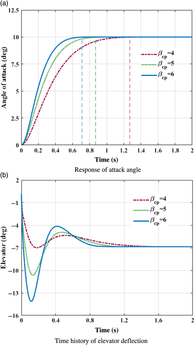
This case simply takes the tracking ability of fixed constant command into consideration. Assume that coefficients of aerodynamic forces and moments are all increased by 30% of their nominal values. First, initial system states and desired commanded signals are set to be α 0 = 0, β 0 = −8, γ 0 = 0, α d = 10, β d = −8, and γd = 45 degree respectively. Figs. 1(a)–3(a) exhibits the time histories of system response in pitch, yaw, and roll channels with different control parameter β cp. Fin deflections in corresponding scenarios are depicted in Figs. 1(b)–3(b).

Figure 1. Control system response in pitch channel. (a) Response of attack angle. (b) Time history of elevator deflection.

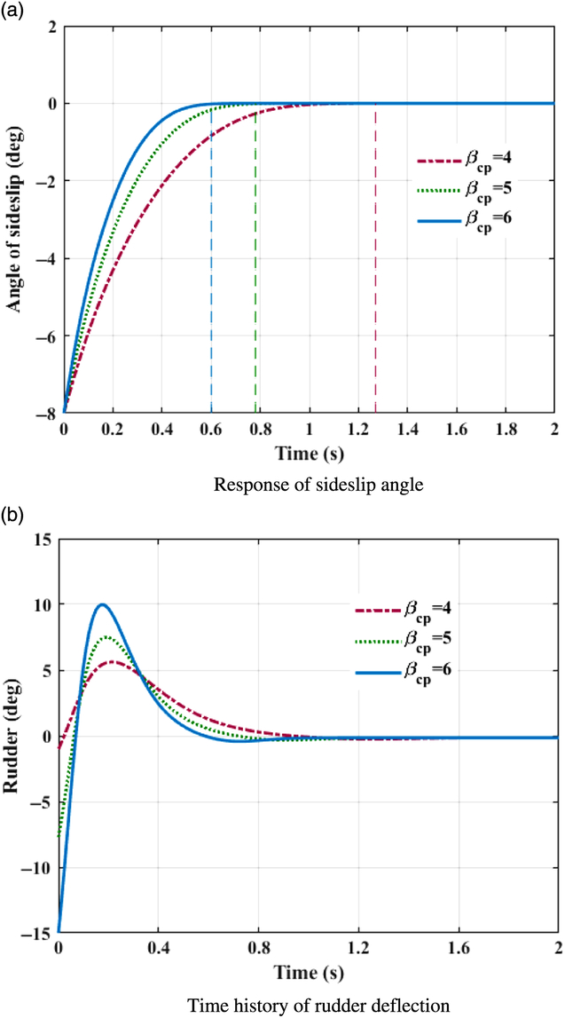
Figure 2. Control system response in yaw channel. (a) Response of sideslip angle. (b) Time history of rudder deflection.
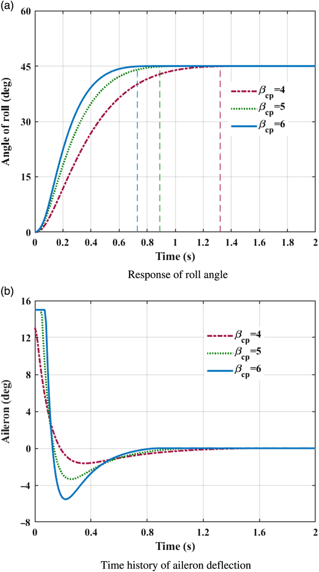
Figure 3. Control system response in roll channel. (a) Response of roll angle. (b) Time history of aileron deflection.
As visualised in Figs. 1(a)–3(a), with the designed controller, BTT missile can track the desired command with satisfactory performance in the presence of nonlinear couplings and aerodynamic uncertainties. The settling times of the angle of attack, sideslip, and roll are approximately summarised in Table 2.
Table 2 Settling time of three channels (s)
Obviously, control variables all converge to their desired value before the theoretical fixed bound of setting time T max, which is calculated from Eq. (35) with the designed parameters. Because of large deviations between command signals and system initial states at the beginning, the control inputs approach large values promptly at initial periods for the sake of tracking. In roll channel as shown in Fig. 3(b), the aileron even goes beyond the deflection constraint. With fin deflections continuously contributing to the control efforts, propelling the required control quantities rapidly within the scope of available control load, the burden of aerodynamic actuator reduced with time increasing, and fins gradually actuate smoothly to ensure the tracking precision. As a result, fast tracking within fixed-bounded convergence time is guaranteed for a BTT missile flight system with the designed controller.
To further validate the fixed-time convergence property of the designed BTT controller, where the fixed bound of settling time is independent of system initial conditions, Monte-Carlo simulations are conducted with various original states, namely, α 0 from −8~16 deg, β0 from −10~10 deg, and γ 0 from −25~45 deg. In this occasion, reference signals are given as α d = 9 deg, β d = 0 deg, and γ d = 25 deg. β cp = 5 and other parameters are identical with previous occasion. The results are depicted in Fig. 4
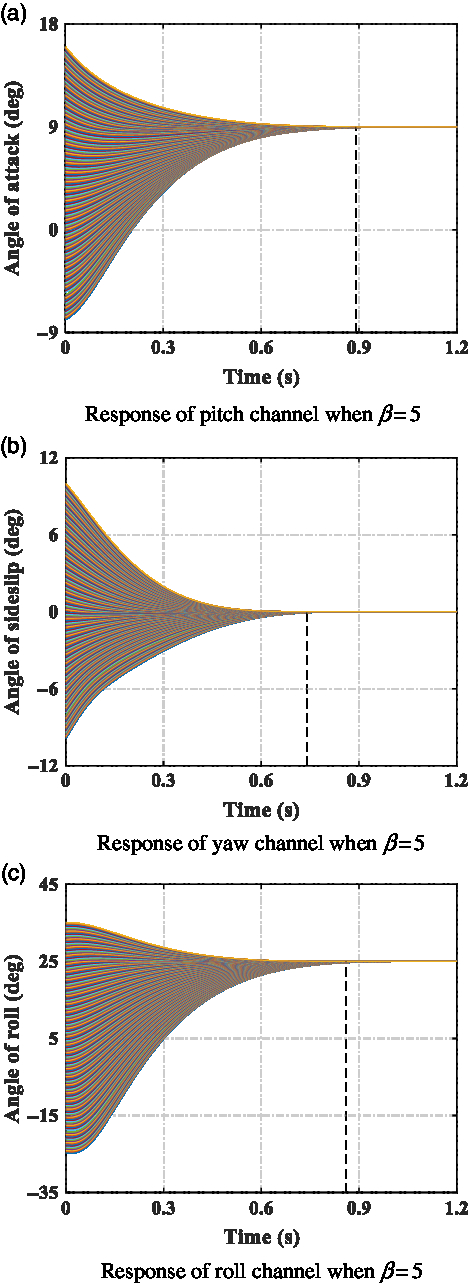
Figure 4. Monte-Carlo simulation with designed BTT controller. (a) Response of pitch channel when β = 5. (b) Response of yaw channel when β = 5. (c) Response of roll channel when β = 5.
Figure 4 sufficiently demonstrates the tracking performance with the designed BTT controller under different initial condition scenarios. A missile can track the desired command before the fixed predefined theoretical bounds of convergence time (T max = 1.27s for β cp = 5). Time histories of system responses exhibit nice uniform convergent characteristic when diverse initial states are given. Simulation results of this situation fully reflect the fixed time convergence characteristic of the designed controller, which is independent of initial conditions and can be evaluated with control parameters in advance. That is also what separates the designed method with conventional terminal sliding-mode controllers.
5.2 Successive command tracking in different aerodynamic uncertainty scenarios
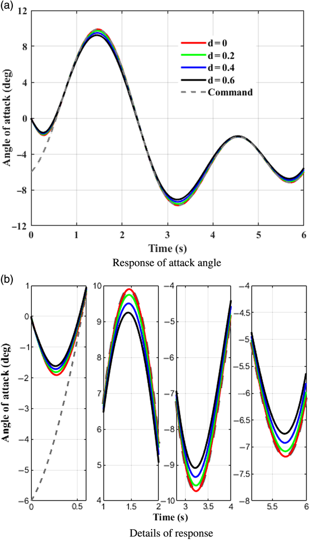
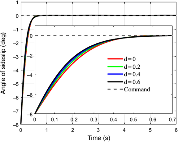
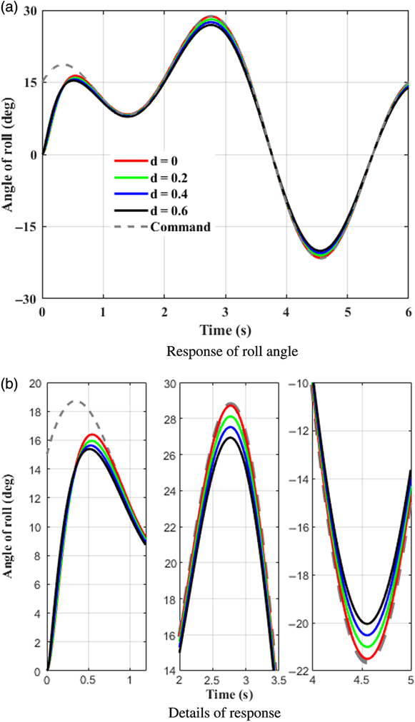
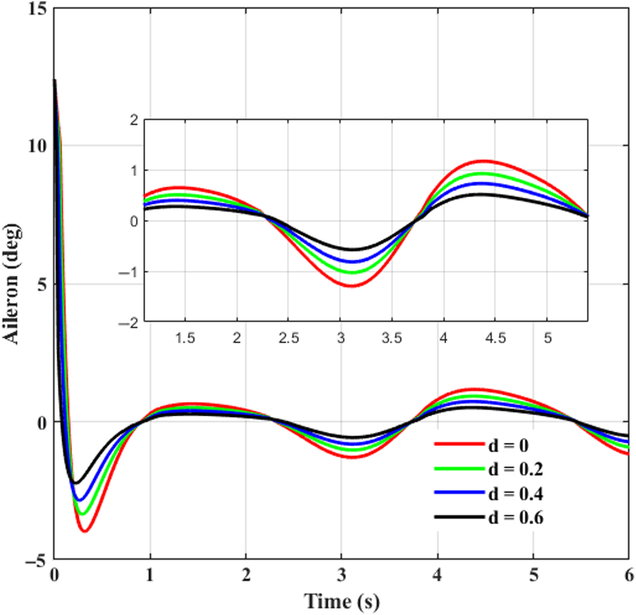
This case takes tracking successive maneuveoringcommand for consideration. A continuous command is generated as the desired signal for BTT missile to maneuveor. It is assumed that aerodynamic coefficients are increased by 20%, 40%, 60%, respectively, that is d α1 = d α2 = d β1= d β2 = d x = d y1 = d y2 = d z1 = d z2 = d, and d = 0.2, 0.4, 0.6. β cp = 5, and initial angle of attack, sideslip, and roll equal to 0, −8, 0 degree, respectively. Time histories of system response with the designed controller in the presence of various uncertainties are depicted in Figs. 5–7, where the continuous turn command are illustrated as a reference. Figures 8–10 give the diagrams of corresponding tail deflections. Details of distinct small deviations have been augmented in subgraphs.

Figure 5. Control system response in pitch channel. (a) Response of attack angle. (b) Details of response.

Figure 6. Control system response in yaw channel.

Figure 7. Control system response in roll channel. (a) Response of roll angle. (b) Details of response.
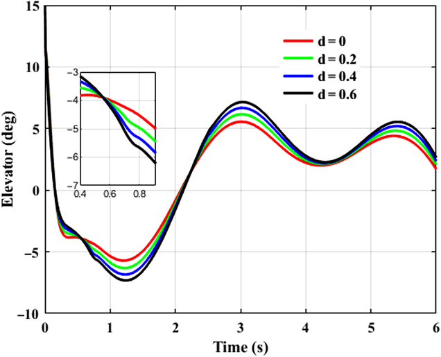
Figure 8. Control time history of elevator deflection.
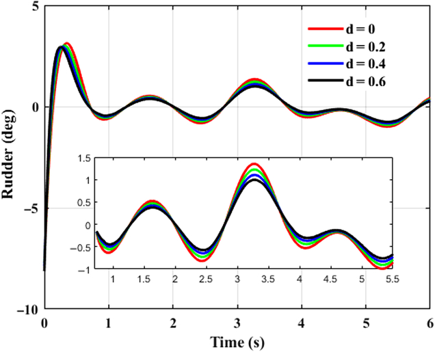
Figure 9. Control time history of rudder deflection.

Figure 10. Control time history of aileron deflection.
Figures 5–7 show that continuous command can be tracked effectively with the designed controller under various aerodynamic uncertainty scenarios. Within theoretical predefined settling time, which is 1.27s, the trajectories of missile attitude angles are driven closely to the desired value at the beginning, and afterwards follows the successive maneuveoringsignal efficiently.
As shown in Figs. 8–10, elevator, rudder, and aileron deflections first increase promptly because of the large deviation between original states and the desired values. When initial errors are swiped out to a small extent, smooth fin deflections take a crucial role consecutively, contributing to effective control efforts and thus improving tracking capacities of missile control system. Despite the fact that command signal in yaw channel is set to be zero, rudder deflection is not zero when corresponding initial error is eliminated as shown in Fig. 9, it deflects coordinately with the other actuators. This is because of the strong nonlinear couplings of BTT missile dynamics. Tracking behaviour in the other directions exerts definite influences on yaw channel, and the inducing effects can be eliminated subsequently with the designed controller. Meanwhile it is worth to notice from Figs. 8–10 that the input signals are smooth without singularity and chattering, which not only enhances tracking performance, but is preferable for practical engineering applications.
Although different degree of aerodynamic uncertainty exists throughout the flight regime, the designed controller guarantees suitable tracking precision of BTT missile flight system and demonstrates satisfactory robustness against uncertainties.
6.0 CONCLUSIONS
This paper designed a robust smooth adaptive sliding-mode-based controller with fixed-time convergence for BTT missiles considering nonlinear couplings and aerodynamic uncertainties. Based on fixed-time stability theory and adaptive estimations, the designed smooth sliding-mode controller guarantees that the BTT missile tracks the commanded angle of attack, sideslip, and roll within fixed bound of setting time under different initial condition scenarios. The bounded convergence rate can be predefined as a function of design parameters regardless of system initial states, which is of significant value from the aspect of preliminary design and performance evaluation. Meanwhile, the smooth controller input representing actuator deflections is intrinsic continuous without adopting any discrete schemes, such that singularity and chattering problems are evaded effectively, facilitating practical implementations of the proposed method as well. In the end, extensive simulations validate the effectiveness of the designed BTT controller.