2.1 Modeling

In the current work, Fig. 1 has shown a scenario where an interception missile is approaching a maneuvering target. M denotes the missile while T denotes the target, the distance from M to T is denoted by R. The line-of-sight (LOS) angle between M and T is λ, and V _M denotes the velocity of M while V _T denotes the velocity of T Moreover, the accelerations of M and T are denoted by A _M and A _T, respectively. Meanwhile, the flight path angles of M and T are denoted by γ _M and γ _T, respectively.

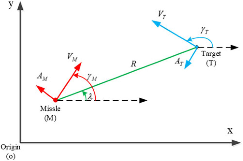
Figure 1. Schematic of terminal homing engagement.

Assuming the velocities of M and T are non-varying and have constant values, the M-T relative kinematics of the engagement can be formulated from^{(Reference He, Lin and Wang14)}

(1) \begin{equation} \dot{R}=V_{T} \cos (\gamma _{T} -\lambda )-V_{M} \cos (\gamma _{M} -\lambda ) \lt 0 \end{equation}

(2) \begin{equation} \dot{\lambda }=\frac{1}{R} [V_{T} \sin (\gamma _{T} -\lambda )-V_{M} \sin (\gamma _{M} -\lambda )] \end{equation}

(3) \begin{equation} \dot{\gamma }_{M} =\frac{A_{M} }{V_{M} } \end{equation}

(4) \begin{equation} \dot{\gamma }_{T} =\frac{A_{T} }{V_{T} } \end{equation}

From Eq. (1) and Eq. (2) ^{(Reference He, Lin and Wang14)}, the derivative of ${\dot{R}}$ and ${\dot{\lambda }}$ can be derived as follows:

(5) \begin{equation} \ddot{R}=R\dot{\lambda }^{2} +A_{TR} -A_{M} \sin (\lambda -\gamma _{M} )\end{equation}

(6) \begin{equation}\ddot{\lambda }=-\frac{2 \dot{R}\dot{\lambda }-A_{T\lambda } +A_{M} \cos (\lambda -\gamma _{M} )}{R}\end{equation}

where ${A_{TR} =A_{T} \sin (\lambda -\gamma _{T} )}$ represents the target’s acceleration along the LOS, and ${A_{T\lambda } =A_{T} \cos (\lambda -\gamma _{T} )}$ represents the target’s acceleration normal to the LOS. Here, a new variable h is defined as:

(7) \begin{equation} h=A_{M} +A_{T\lambda } -A_{M} \cos (\lambda -\gamma _{M} )\end{equation}

Consequently, the angle rate dynamics from Eq. (6) of the LOS can be rewritten as

(8) \begin{equation} \ddot{\lambda }=-\frac{2 \dot{R}\dot{\lambda }-h+A_{M} }{R} \end{equation}

On account of the non-cooperative nature of the target, A _Tλ is obviously unknown for the interception missile in advance. Therefore, the variable h can be taken as a model uncertainty and can be assumed to be bounded with the form as^{(Reference He, Lin and Wang14)}:

(9) \begin{equation} \left|\frac{d^{ j} h}{dt^{ j} } \right|\le \mu \; \; \; j=0,{\rm \; }1,{\rm \; }2,{\rm \; }...,{\rm \; }n \end{equation}

where μ is an unknown positive constant.

2.2 The linear sliding mode manifold for the state errors

Considering a system such as

(10) \begin{equation} \ddot{x}=f(x,\dot{x},t)+g(x,\dot{x},t)u \end{equation}

In Eq. (10), ${f(x,\dot{x},t)}$ and ${g(x,\dot{x},t)}$ are known functions, u is the control input.

A linear sliding mode manifold can be defined as^{(Reference Liu and Wang16)}:

(11) \begin{equation} s_{x} = \dot{x}+kx=0,\; \; k \gt 0 \end{equation}

where s _x is a sliding mode variable. If ${s_{x} =0}$ , the system states x and ${\dot{x}}$ will be asymptotically driven to zero^{(Reference Liu and Wang16)}.

As stated in the literatures^{(Reference Lyu and Zhu17,Reference Lyu, Zhu, Tang and Yan18)} , the interception guidance law for a missile determines the guidance commands needed to control the missile to capture the target with a predesigned LOS angle ${\lambda _{d} }$ if the value of R is lower than a constant value ${R_{f} }$ . Accordingly, the LOS angle error of the missile is yielded as ${e_{\lambda } =\lambda -\lambda _{d} }$ . Moreover, the angle error dynamics is yielded by as per the literatures^{(Reference Lyu and Zhu17,Reference Lyu, Zhu, Tang and Yan18)}

(12) \begin{equation} \ddot{e}_{\lambda } =\ddot{\lambda }=-\frac{2 \dot{R}\dot{\lambda }-h+A_{M} }{R} \end{equation}

According to Eq. (11), a sliding mode variable can be determined as:

(13) \begin{equation} s_{e} = \dot{e}_{\lambda } +ke_{\lambda } \end{equation}

and its derivative is yielded as

(14) \begin{equation} \dot{s}_{e} =\ddot{e}_{\lambda } +k \dot{e}_{\lambda } =-\frac{2 \dot{R}\dot{\lambda }-h+A_{M} }{R} +k \dot{e}_{\lambda }\end{equation}

3.1 PPC and IDC-based guidance law (PIGL)

Since the performance of guidance commands is coupled to the convergence rate of the sliding mode variable, a prescribed performance controller with a revised PPF, which inherits the initial time-varying properties of the sliding mode variable, can enhance the transient performance of commands, such as, avoiding large sudden changes in the guidance commands. Accordingly, an equivalent second-order system can be constructed as^{(Reference Grinfeld and Ben-Asher19)}:

(15) \begin{equation} \left\{\begin{array}{l} {\dot{\rho }=u_{\rho } } \\ {\dot{u}_{\rho } =u_{jerk} } \end{array}\right. \end{equation}

where ρ is the prescribed performance variable (PPV) and is treated as an equivalent system state, ${u_{\rho } }$ is the virtual control command and is also treated as another equivalent system state, ${u_{jerk} }$ represents the virtual jerk. An optimal cost function can be defined as follows:

(16) \begin{equation} \min \; J=\int _{0}^{t_{d} }{\left(\left(t-t_{d} /\beta \right)^{2} +1\right)^{-1} u_{jerk}^{2} \mathord{\left/ {\vphantom {\left(\left(t-t_{d} /\beta \right)^{2} +1\right)^{-1} u_{jerk}^{2} 2}} \right. } 2} dt \end{equation}

where t _d is a predetermined time, and β is a weighting parameter used to adjust the characteristics of u _ρ. The boundary conditions of the equivalent second-order system are ${\left. \rho \right|_{t=0} =s_{0} },{\left. \rho \right|_{t=t_{d} } =s_{d} },{\left. u_{\rho } \right|_{t=0} =u_{\rho 0} }$ , ${\left. u_{\rho } \right|_{t=t_{d} } =u_{\rho d} }$ , where s ₀ is the initial value of s _e, ${u_{\rho 0} }$ is the initial value of the approximate derivative of the sliding mode variable ${\dot{\hat{s}}_{e} }$ without considering the unknown uncertainty h, ${u_{\rho d} }$ is the predesigned virtual control command at ${t=t_{d} }$ , and s _d is a predetermined value of s at ${t=t_{d} }$ .

The Hamilton function of the optimal problem can be written as:

(17) \begin{equation} H=\lambda _{\rho } u_{\rho } (t)+\lambda _{u_{\rho } } u_{jerk} +\left(\left(t-t_{d} /\beta \right)^{2} +1\right)^{-1} u_{jerk}^{2} /2 \end{equation}

where ${\lambda _{\rho } }$ and ${\lambda _{u_{\rho } } }$ are covariant variables.

As per the literature^{(Reference Bryson, Ho and Siouris20)}, the solutions are as follows:

(18) \begin{equation} \dot{\lambda }_{\rho } =-\frac{\partial H}{\partial \rho } =0\Rightarrow \lambda _{\rho } =a_{1} \end{equation}

(19) \begin{equation}\dot{\lambda }_{u_{\rho } } =-\frac{\partial H}{\partial u_{\rho } } =-\lambda _{\rho } \Rightarrow \lambda _{u_{\rho } } =-a_{1} t+a_{2} \end{equation}

(20) \begin{equation} \frac{\partial H}{\partial u_{jerk} } =\left(\left(t-t_{d} /\beta \right)^{2} +1\right)^{-1} u_{jerk} +\lambda _{u_{\rho } } =0\Rightarrow u_{jerk} =-\left(\left(t-t_{d} /\beta \right)^{2} +1\right)\lambda _{u_{\rho } }\end{equation}

Consequently, the general solutions for ${u_{\rho } }$ and ${\rho }$ are as follows:

(21) \begin{equation} \begin{array}{l} {u_{\rho } =a_{3} -\bigg(a_{2} +\frac{a_{2} t_{d}^{2} }{\beta ^{2} } \bigg)t+\left(\frac{a_{1} }{2} +\frac{a_{2} t_{d} }{\beta } +\frac{a_{2} t_{d}^{2} }{2\beta ^{2} } \right)t^{2} } \\ {\; \; \; \; \; \; \; \; \; \; \; \; \; \; \; \; -\left(\frac{a_{2} }{3} +\frac{2a_{1} t_{d} }{3\beta } \right)t^{3} +\frac{a_{1} t^{4} }{4} } \end{array}\end{equation}

(22) \begin{equation}\begin{array}{l} {\rho =a_{4} +a_{3} t-\frac{1}{2} \left(a_{2} +\frac{a_{2} t_{d}^{2} }{\beta ^{2} } \right)t^{2} +\frac{1}{3} \left(\frac{a_{1} }{2} +\frac{a_{2} t_{d} }{\beta } +\frac{a_{2} t_{d}^{2} }{2\beta ^{2} } \right)t^{3} } \\[-7pt] {\; \; \; \; \; \; \; \; \; -\frac{1}{4} \left(\frac{a_{2} }{3} +\frac{2a_{1} t_{d} }{3\beta } \right)t^{4} +\frac{a_{1} t^{5} }{20} }\end{array}\end{equation}

Accordingly, with t increasing from 0 to t _d, the coefficients a ₁, a ₂, a ₃ and a ₄ are determined by the boundary conditions of ${u_{\rho } }$ and ρ.

A transformed error z can be defined as follows^{(Reference Song, Zhang, Zhang and Lu1)}.

(23) \begin{equation} z=\ln \left(\frac{s_{e} /\rho -M_{\min } }{M_{\max } -s_{e} /\rho } \right) \end{equation}

where ${M_{\max } >2}$ and ${M_{\min } =2-M_{\max } }$ . When s ₀ and s _d are nonzero and they both have the same sign, an appropriate value of β in Eq. (22) should be chosen to avoid ρ being zeroed in Eq. (23). In reality, at the beginning of terminal homing phase, s ₀ always satisfies or could be controlled as ${\left|s_{0} \right|\ge \varepsilon _{s} }$ , where ${\varepsilon _{s} }$ has a small positive value.

In Eq. (23), if z asymptotically converges to zero, s _e will also asymptotically converge to ρ. The derivative of z is yielded as follows:

(24) \begin{equation} \dot{z}=\frac{C}{\rho ^{2} } (\dot{s}_{e} \rho -\dot{\rho }s_{e} )\end{equation}

where

(25) \begin{equation} C=\frac{M_{\max } -M_{\min } }{(s_{e} /\rho -M_{\min } )(M_{\max } -s_{e} /\rho )} \end{equation}

A Lyapunov function ν can be constructed as:

(26) \begin{equation} \nu =\frac{1}{2} z^{2}\end{equation}

Substituting Eq. (12) and Eq. (14) into Eq. (24) yields ${\dot{z}}$ as follows:

(27) \begin{equation} \dot{z}=\frac{C}{\rho ^{2} } \left[\left(-\frac{2 \dot{R}\dot{\lambda }-h+A_{M} }{R} +k \dot{e}_{\lambda } \right)\rho -\dot{\rho }s_{e} \right] \end{equation}

A _M can be defined as:

(28) \begin{equation} A_{M} =-R\left(u_{eq_{1} } +\frac{\rho }{C} u_{2} \right) \end{equation}

where

(29) \begin{equation} u_{eq_{1} } =\frac{2 \dot{R}\dot{\lambda }}{R} +\frac{\dot{\rho }}{\rho } s_{e} -k \dot{e}_{\lambda } \end{equation}

and h ₁ can be defined as:

(30) \begin{equation} h_{1} =\frac{Ch}{\rho R}\end{equation}

Substituting Eqs. (28), (29) and (30) into Eq. (27), the revised term ${\dot{z}}$ is yielded as follows:

(31) \begin{equation} \dot{z}=h_{1} +u_{2} \end{equation}

h ₁ is passed through a broadband filter G _f(s), such as^{(Reference Phadke and Talole13)}:

(32) \begin{equation} G_{f} (s)=\frac{1}{\tau s+1}\end{equation}

where τ is a constant. The dynamics of the estimate of h ₁ is yielded as:

(33) \begin{equation} \tau \dot{\hat{h}}_{1} +\hat{h}_{1} =\dot{z}-u_{2} \end{equation}

If u ₂ is designed as

(34) \begin{equation} u_{2} =-k_{z} z-\hat{h}_{1} \end{equation}

Then Substituting Eq. (34) into Eq. (33) yields the following:

(35) \begin{equation} \tau \dot{\hat{h}}_{1} =\dot{z}+k_{z} z \end{equation}

Integrating both sides of Eq. (35) yields the following:

(36) \begin{equation} \hat{h}_{1} =\left. \hat{h}_{1} \right|_{t=0} +\frac{1}{\tau } \left(z-\left. z\right|_{t=0} +\int _{0}^{t}k_{z} zdt \right) \end{equation}

As ${\left. \rho \right|_{t=0} =s_{0} }$ , as per Eq. (23), ${\left. z\right|_{t=0} }$ is zero. Accordingly, Eq. (36) can be revised as:

(37) \begin{equation} \hat{h}_{1} =\left. \hat{h}_{1} \right|_{t=0} +\frac{1}{\tau } \left(z+\int _{0}^{t}k_{z} zdt \right)\end{equation}

By substituting Eqs. (29), (34) and (37) into Eq. (28), the PPC and IDC-based guidance law are yielded as follows.

(38) \begin{equation} A_{M} =-R\left(\frac{2 \dot{R}\dot{\lambda }}{R} +\frac{\dot{\rho }}{\rho } s_{e} -k \dot{e}_{\lambda } -\frac{\rho }{C} \left(k_{z} z+\left. \hat{h}_{1} \right|_{t=0} +\frac{1}{\tau } \left(z+\int _{0}^{t}k_{z} zdt \right)\right)\right)\end{equation}

In order to avoid A _m having large and discontinuous changes at the initial time, ${\left. \hat{h}_{1} \right|_{t=0} }$ is necessary to be predesigned. Assuming ${\left. A_{M} \right|_{t=0^{-} } }$ is known, then, ${\left. A_{M} \right|_{t=0^{+} } }$ can be subsequently determined from Eq. (38) as:

(39) \begin{equation} \left. A_{m} \right|_{t=0^{+} } =\left. A_{m} \right|_{t=0^{-} } +\left. R\right|_{t=0^{+} } \left. \hat{h}_{1} \right|_{t=0} +\left. \varepsilon \right|_{t=0^{+} }\end{equation}

where ${\left. \varepsilon \right|_{t=0^{+} } }$ is a small value. Then, ${\left. \hat{h}_{1} \right|_{t=0} }$ should be zeroed; then, Eq. (38) should be revised to:

(40) \begin{equation} A_{M} =-R\left(\frac{2 \dot{R}\dot{\lambda }}{R} +\frac{\dot{\rho }}{\rho } s_{e} -k \dot{e}_{\lambda } -\frac{k_{z} z\rho }{C} -\frac{\rho }{C\tau } \left(z+\int _{0}^{t}k_{z} zdt \right)\right)\end{equation}

Then, the proposed guidance law (PIGL) which integrates PPC and IDC can be obtained from Eq. (40).

Next, the stability and robustness of the system from Eq. (24) has been analyzed by applying PIGL from Eq. (38).

By substituting Eq. (38) into Eq. (27), the derivative of z can be obtained as:

(41) \begin{equation} \dot{z}=-k_{z} z+\big(h_{1} -\hat{h}_{1} \big)\end{equation}

Then ${\tilde{h}_{1} =h_{1} -\hat{h}_{1} }$ can be defined and the derivative of ${\tilde{h}_{1} }$ is obtained as

(42) \begin{equation} \dot{\tilde{h}}_{1} =-\tau ^{-1} \tilde{h}_{1} +\dot{h}_{1}\end{equation}

A Lyapunov function ${\nu \big(z,\tilde{h}_{1} \big)}$ can be constructed as

(43) \begin{equation} \nu \big(z,\tilde{h}_{1} \big)=\frac{1}{2} z^{2} +\frac{1}{2} \tilde{h}_{1}^{2} \end{equation}

Substituting Eqs. (41) and (42) into the derivative of ${\nu \big(z,\tilde{h}_{1} \big)}$ , ${\dot{\nu }\big(z,\tilde{h}_{1} \big)}$ yields the following:

(44) \begin{equation} \begin{array}{l} {\dot{\nu }\big(z,\tilde{h}_{1} \big)=-k_{z} z^{2} +\tilde{h}_{1} z-\tau ^{-1} \tilde{h}_{1}^{2} +\tilde{h}_{1} \dot{h}_{1} } \\ {\; \; \; \; \; \; \; \; \; \; \; \; \; \; \; \; \; \le -\left(k_{z} -1/2\right)z^{2} -\left(\tau ^{-1} -1\right)\tilde{h}_{1}^{2} +\dot{h}_{1}^{2} }\end{array}\end{equation}

From Eq. (9) and Eq. (30), it can be seen that ${\dot{h}_{1}^{2} }$ is bounded. Therefore, the necessary conditions which assure ${\nu \big(z,\tilde{h}_{1} \big)}$ converges to a boundary region around zero are ${k_{z} \gt 1/2}$ and ${0 \lt \tau \lt 1}$ . z is substantially bounded at ${t=t_{d} }$ , and ${\left. s_{e} \right|_{t=t_{d} } }$ could converge to a small region around s _d^{(Reference Bechlioulis and Rovithakis21)}.

3.2 SMC and IDC-based guidance law (SIGL)

PIGL is capable of controlling both the LOS angle and its rate to a small region without an abrupt command altering it under the unknown uncertainty induced by the target’s maneuvers. However, it is not able to accurately drive the LOS angle and LOS angle rate to the desired value. Here, a SMC and IDC-based guidance law (SIGL) has been proposed to implement the final convergence of both the LOS angle and its rate.

The auxiliary variable σ ^{(Reference Phadke and Talole13)} can be defined as:

(45) \begin{equation} \sigma =s_{e} +z_{s} ,\; \; \; \left. z_{s} \right|_{t=t_{0} } =-\left. s_{e} \right|_{t=t_{0} } \end{equation}

Where, t ₀ is the initial time when SMC and IDC-based guidance law are applied and the derivative of z _s is as follows:

(46) \begin{equation} \dot{z}_{s} =k_{s} s_{e} +l_{s} \left(t-t_{0} \right)sign(s_{e} )\end{equation}

where k _s is a positive value and l _s is a small positive value.

Consequently, by substituting Eqs. (12), (14) and (46) into the derivative of σ yields ${\dot{\sigma }}$ as follows.

(47) \begin{equation} \dot{\sigma }=-\frac{2 \dot{R}\dot{\lambda }-h+A_{M} }{R} +k \dot{e}_{\lambda } +k_{s} s_{e} +l_{s} \left(t-t_{0} \right)sign(s_{e} ) \end{equation}

A _M can be defined as:

(48) \begin{equation} A_{M} =-R(u_{eq} +u_{1} ) \end{equation}

where

(49) \begin{equation} u_{eq} =\frac{2 \dot{R}\dot{\lambda }}{R} -\left(k \dot{e}_{\lambda } +k_{s} s_{e} +l_{s} (t-t_{0} )sign(s_{e} )\right) \end{equation}

and h ₁ can be defined as follows:

(50) \begin{equation} h_{2} =\frac{h}{R} \end{equation}

Accordingly, substituting Eqs. (48), (49) and (50) into Eq. (47) yields h ₂ as follows.

(51) \begin{equation} h_{2} =\dot{\sigma }-u_{1} \end{equation}

If h ₂ is passed through a broadband filter G _f(s) from Eq. (32), then, the dynamics of the estimate of h ₂ is yielded as

(52) \begin{equation} \tau \dot{\hat{h}}_{2} +\hat{h}_{2} =\dot{\sigma }-u_{1}\end{equation}

u ₁ can be designed as:

(53) \begin{equation} u_{1} =-k_{\sigma } \sigma -\hat{h}_{2}\end{equation}

Substituting Eq. (53) into Eq. (52) yields ${\dot{\hat{h}}_{2} }$ as follows.

(54) \begin{equation} \dot{\hat{h}}_{2} =\tau ^{-1} \left(\dot{\sigma }+k_{\sigma } \sigma \right)\end{equation}

Integrating both sides of Eq. (54) yields ${\hat{h}_{2} }$ as follows.

(55) \begin{equation} \hat{h}_{2} =\left. \hat{h}_{2} \right|_{t=t_{0} } +\frac{1}{\tau } \left(\sigma +\int _{t_{0} }^{t}k_{\sigma } \sigma dt \right)\end{equation}

Accordingly, the SMC and IDC-based guidance law (SIGL) are yielded as follows

(56) \begin{equation} \begin{array}{l} {A_{M} =-R\bigg(\frac{2 \dot{R}\dot{\lambda }}{R} -\left(k \dot{e}_{\lambda } +k_{s} s_{e} +l_{s} (t-t_{0} )sign(s_{e} )\right)} \\ {\; \; \; \; \; \; \; \; \; \; \; \; \; \; \; \; \; \; \; \; \; \; \; \; \; \; \; \; \; \; \; \; -\left(k_{\sigma } +\frac{1}{\tau } \right)\sigma -\left. \hat{h}_{2} \right|_{t=t_{0} } -\frac{1}{\tau } \displaystyle\int _{t_{0} }^{t}k_{\sigma } \sigma dt \bigg)} \end{array}\end{equation}

Next, the stability and robustness of the system from Eq. (45) by applying SIGL from Eq. (56) has been analyzed.

Substituting Eq. (56) into Eq. (47), the derivative of σ is yielded as

(57) \begin{equation} \dot{\sigma }=-k_{\sigma } \sigma +\big(h_{2} -\hat{h}_{2} \big)\end{equation}

Defining ${\tilde{h}_{2} =h_{2} -\hat{h}_{2} }$ and the derivative of ${\tilde{h}_{2} }$ can be written as:

(58) \begin{equation} \dot{\tilde{h}}_{2} =-\tau ^{-1} \tilde{h}_{2} +\dot{h}_{2}\end{equation}

A Lyapunov function ${\nu \big(\sigma ,\tilde{h}_{2} \big)}$ can be constructed as

(59) \begin{equation} \nu \big(\sigma ,\tilde{h}_{2}\big)=\frac{1}{2} \sigma ^{2} +\frac{1}{2} \tilde{h}_{2}^{2}\end{equation}

Substituting Eq. (57) and Eq. (58) into the derivative of ${\nu \big(\sigma ,\tilde{h}_{2}\big)}$ yields ${\dot{\nu }\big(\sigma ,\tilde{h}_{2}\big)}$ as follows.

(60) \begin{equation} \begin{array}{l} {\dot{\nu }\big(\sigma ,\tilde{h}_{2}\big)=-k_{\sigma } \sigma ^{2} +\tilde{h}_{1} \sigma -\tau ^{-1} \tilde{h}_{2}^{2} +\tilde{h}_{2} \dot{h}_{2} } \\ {\; \; \; \; \; \; \; \; \; \; \; \; \; \; \; \; \; \; \le -\left(k_{\sigma } -1/2\right)\sigma ^{2} -\left(\tau ^{-1} -1\right)\tilde{h}_{2}^{2} +\dot{h}_{2}^{2} } \end{array}\end{equation}

As per Eqs. (9) and (50), ${\dot{h}_{2}^{2} }$ is bounded, the necessary conditions where ${\nu \big(\sigma ,\tilde{h}_{2}\big)}$ converges to a boundary region are ${k_{\sigma } \gt 1/2}$ and ${0 \lt \tau \lt 1}$ .

Furthermore, a Lyapunov function ${\nu _{s_{e} } }$ can be defined as

(61) \begin{equation} \nu _{s_{e} } =\frac{1}{2} s_{e}^{2}\end{equation}

Substituting Eqs. (46) and (57) into the derivative of ${\nu _{s_{e} } }$ yields ${\dot{\nu }_{s_{e} } }$ as follows.

(62) \begin{equation} \begin{array}{l} {\dot{\nu }_{s_{e} } =s_{e}^{} \big(-k_{s} s_{e} -l_{s} (t-t_{0} )sign(s_{e} )-k_{\sigma } \sigma +\tilde{h}_{2} \big)} \\ {\; \; \; \; \; \; \le -2k_{s} V_{s_{e} } -\sqrt{2} \Big(l_{s} (t-t_{0} )-\left|k_{\sigma } \sigma \right|-\left|\tilde{h}_{2} \right|\Big)V_{s_{e} }^{1/2} } \end{array}\end{equation}

Since ${\left|\sigma \right|}$ and ${\left|\tilde{h}_{2} \right|}$ are bounded, ${\left|\sigma \right|\le \left|\sigma \right|_{\max } }$ and ${\left|\tilde{h}_{2} \right|\le \left|\tilde{h}_{2} \right|_{\max } }$ can be defined. Theoretically, different values of l _s exist, if ${t_{f} \gt t \ge t_{s} \gt t_{0} }$ , $\left. l_{s} \left(t-t_{0} \right)\right|_{t>t_{s} } =\upsilon +\left|\sigma \right|_{\max } +$ $\left|\tilde{h}_{2} \right|_{\max } $ , where ${t_{f} }$ denotes the terminal guidance time. Accordingly, if ${t_{f} \gt t \ge t_{s} \gt t_{0} }$ , then Eq. (62) can be revised as follows:

(63) \begin{equation} \left. \dot{\nu }_{s_{e} } \right|_{t \gt t_{s} } \le \left. -2k_{s} \nu _{s_{e} } \right|_{t \gt t_{s} } -\left. \sqrt{2} \upsilon \nu _{s_{e} }^{1/2} \right|_{t \gt t_{s} }\end{equation}

As per the literature^{(Reference Hong, Huang and Xu22)}, ${\nu _{s_{e} } }$ will converge to zero in a finite time; consequently, ${s_{e} }$ converges to zero in a finite time. Furthermore, ${e_{\lambda } }$ and ${ \dot{e}_{\lambda } }$ will asymptotically converge to zero.

3.3 The hybrid strategy

Considering the strengths and weaknesses of both PIGL and SIGL, a hybrid guidance strategy has been proposed here to capture a non-cooperative maneuvering target without knowing the uncertainty h in advance. The guidance strategy for the terminal homing phase consists of two phases.

In the first phase, the PIGL guidance law is adopted to control s _e in a small predesigned range without large and abrupt changes of the guidance commands in a fixed time t _d, where ${t_{d} =t_{go_{0} } -t_{switch} }$ . ${t_{go_{0} } }$ is the initial estimated time-to-go between the missile and the target, and determined by ${t_{go_{0} } \approx {-\left. R\right|_{t=0} \mathord{\left/ {\vphantom {-\left. R\right|_{t=0} \left. \dot{R}\right|_{t=0} }} \right. } \left. \dot{R}\right|_{t=0} } }$ . t _switch is a predetermined time point, at which, the PIGL is shifted to SIGL. In order to achieve smooth switching, u _ρd is established as ${-k_{s} s_{d} }$ .

In the second phase, SIGL is applied to guarantee that s _e converges to zero in a finite time in order to pursue high interception accuracy with reduced sensitivity to errors in the estimation of the time-to-go.

From the analysis of both phases, the time-to-go estimation will not be used as per PIGL in Eq. (40) and SIGL in Eq. (56) in the application process. The hybrid guidance law scheme has been shown in Fig. 2.

Figure 2. Hybrid guidance law scheme.

4.1 Comparison with the other guidance laws

The initial simulation conditions have been provided in Table 1. The maneuvering acceleration profile of the target was assumed as ${A_{T} =-4g\sin ({\pi t\mathord{\left/ {\vphantom {\pi t 4}} \right.} 4} )}$ , where ${g=9.8{\rm m/s}^{{\rm 2}} }$ denotes the value of the acceleration du to gravity. The desired terminal LOS angle was ${\lambda _{d} =\pi /6{\rm rad}}$ , and the upper bound of acceleration of interception missiles is assumed to be 20g. For comparison, another two guidance laws were introduced. One was the continuous impact angle homing guidance law in Ref.^{(Reference He and Lin5)}, named S Cont.-SMC for short. The other is a second order sliding mode guidance law with uncertainty and disturbance estimator in Ref.^{(Reference Yamasaki, Balakrishnan, Takano and Yamaguchi6)}, named Est.-SMC for short.

Table 1. Initial values of the missile and the target

Cont.-SMC is represented per the literature as^{(Reference He and Lin5)}:

(64) \begin{equation} A_{M} =\frac{R}{\cos (\lambda -\gamma _{M} )} \left[-\frac{2 \dot{R}\dot{\lambda }}{R} +\frac{q}{\eta p} \left|\dot{\lambda }\right|^{2-\frac{p}{q} } sgmf\left(\dot{\lambda }\right)+\frac{k_{1} }{R} s+\frac{k_{2} }{R} \left|s\right|^{\omega } sgmf\left(s\right)\right] \end{equation}

where

(65) \begin{equation} s=e_{\lambda } +\eta \left| \dot{e}_{\lambda } \right|^{\frac{p}{q} } sign( \dot{e}_{\lambda } )\end{equation}

(66) \begin{equation} sgmf(s)=2\left(\frac{1}{1+\exp (-as)} -\frac{1}{2} \right)\!,\; \; \; a \gt 0 \end{equation}

Est.-SMC is represented per the literature as^{(Reference Yamasaki, Balakrishnan, Takano and Yamaguchi6)}:

(67) \begin{equation} A_{M} =u_{e} +u_{s} +\hat{h} \end{equation}

where

(68) \begin{equation} u_{e} =-(k_{3} +k_{4} +2) \dot{R}\dot{\lambda }-\frac{(k_{4} +1)k_{3} }{t_{go} } \dot{R}\left(\lambda -\lambda _{d} \right) \end{equation}

(69) \begin{equation}u_{s} =-R\left\{-b_{1} \left|\kappa \right|^{\alpha _{1} } sign(\kappa )+w\right\}\end{equation}

(70) \begin{equation}\hat{h}=(R\kappa +w_{2} )/\tau _{m}\end{equation}

(71) \begin{equation}\left\{\begin{array}{l} {\kappa =s_{b} +m_{z} ,\; \left. m_{z} \right|_{t=0} =-\left. s_{b} \right|_{t=0} } \\ {s_{b} =\dot{\lambda }+k_{3} \frac{\lambda -\lambda _{d} }{t_{go} } }\\ {\dot{m}_{z} =\frac{k_{4} s_{b} }{t_{go} } } \\ {\begin{array}{l} {\dot{w}=-b_{2} \left|\kappa \right|^{\alpha _{2} } sign(\kappa )} \\ {\dot{w}_{2} =- \dot{R}\kappa +u_{s} } \end{array}} \end{array}\right.\end{equation}

The parameters of the proposed Hybrid guidance law were assigned as k = 30, ${k_{s} =1.0},{l_{s} =1.0\times 10^{-3} },{M_{\min } =-2}, {M_{\max } =4},{k_{\sigma } =k_{z} =2},{\tau =0.05s},{\beta =0.01},{t_{switch} =8s}, {\left. s_{e} \right|_{t=t_{d} } =s_{0} /50}$ .

The parameters for the Cont.-SMC guidance law were η = 1, p = 21, q = 19, k ₁ = 60, k ₂ = 400, ω = 0.5, a = 100.

The values of the parameter for the Est.-SMC guidance law were k ₃ = 3, k ₄ = 1.5, b ₁ = 1, b ₂ = 1, α ₁ = 0.7, α ₂} = 0.7, τ _m = 0.05s.

To avoid chattering in the guidance commands caused by the discontinuous signum function, a saturation function sat(x) was used to address the problem as per the literature^{(Reference He, Lin and Wang14)}:

(72) \begin{equation} sat(x)=\left\{\begin{array}{l} {sign(x),\; \; \; \; \left|x\right|>\vartheta } \\[4pt] {x/\vartheta ,\; \; \; \; \; \; \; \; \left|x\right|\le \vartheta } \end{array}\right.\end{equation}

Where, ${\vartheta }$ is a small positive constant and was selected as 0.001. The simulation step was 2ms, and the simulation was terminated when ${R\le R_{f} =20{\rm m}}$ .

The results of simulation have been shown in Fig. 3. The terminal guidance errors have been listed in Table 2. Figure 3(a) has shown the trajectories of the missile during the terminal homing interception phase. The curvatures of the trajectories at the beginning of the terminal homing phase generated by Cont.-SMC and Est.-SMC were greater than that for the Hybrid guidance law. Meanwhile, the commanded accelerations of the missile have been shown in Fig. 2(b). The largest acceleration in the initial homing phase determined by Hybrid guidance law was smaller than the other two guidance laws. Figure 3(c) and (d) indicate that the terminal LOS angle and its rate finally converged rapidly to the desired value and around zero, respectively. During the convergence phase, the LOS angle and the LOS angle rate yielded by the Hybrid guidance law were not affected by target’s maneuvers, while those from the other two guidance law were deeply affected by target’s maneuver. Compared with Cont.-SMC and Est.-SMC, the values of the LOS angle and the LOS angle rate reached zero more quickly and could stay in small regions around zero. In Fig. 3(e), the sliding mode variable determined by the hybrid guidance law could be driven into the predesigned region at a fixed time and converged to zero to pursue high terminal interception precision. Even though the time-to-go is not used by the Hybrid guidance law, the terminal interception precision can be guaranteed as the performance of the Est.-SMC guidance law.

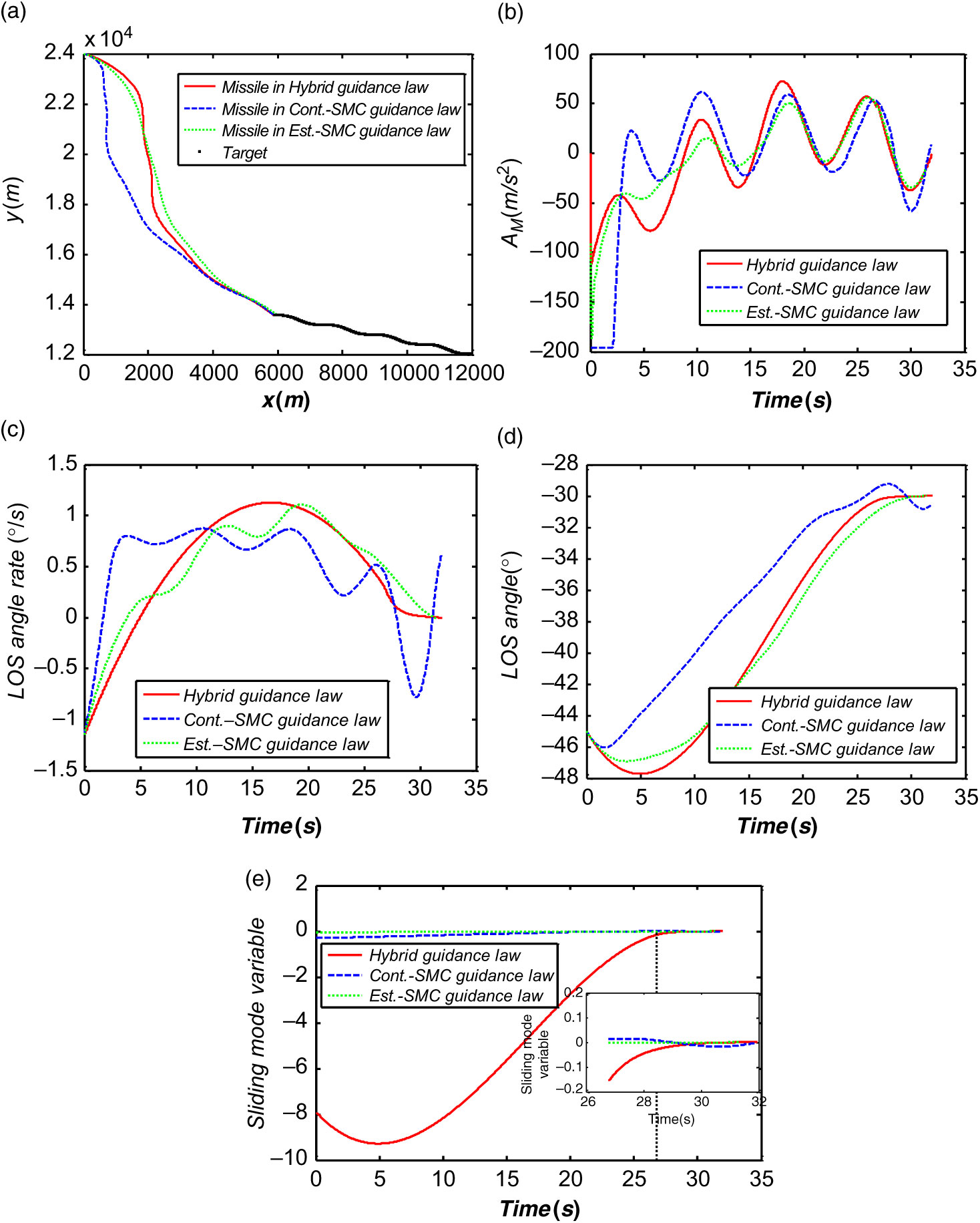
Figure 3. Comparison results from the Hybrid guidance law, the Cont.-SMC guidance law and the Est.-SMC guidance law: a) interception trajectories, b) the accelerations the missile achieved, c) the LOS angle rate, d) the LOS angle, e) the sliding mode variables.

Table 2. Terminal guidance errors

4.2 Performance test

In order to verify the robustness and performance of the proposed guidance law, Monte Carlo simulation with 100 cases was then carried out. The dispersion of the parameters for the Monte Carlo simulation has been listed in Table 3. Moreover, the dominated control gain k _z, assumed to be loosely chosen in boundary regions, was dealt with as an uncertainty.

Table 3. Lower and upper bounds for the uncertainty parameters

Figure 4(a) has shown the acceleration commands of the missile under different initial states and for various values of the control gain k _z. It also indicates that large abrupt changes in the beginning period were eliminated notwithstanding the initial states, and that the control gain k _z varied. Therefore, it demonstrated one critical advantage where the yielded guidance commands were insensitive to the initial state errors between the initial states and the desired states as well as the uncertainty caused by the target’s maneuvers. Figure 4(b) and (c) have depicted the scatter of the terminal LOS angle error and the LOS angle rate error of the missile, they have demonstrated that the proposed guidance law has a good robustness in guaranteeing the convergent accuracy of the LOS angle and the LOS angle rate errors. Figure 4(d) has depicted the zero-effort miss between the missile and the target; it reflects that fact that the proposed robust hybrid nonlinear guidance law can guide the missile to achieve high interception accuracy. Subsequently, another advantage, where it loosely chooses the control gain k _z without acquiring the uncertainties in advance, has been demonstrated by this numerical simulation.

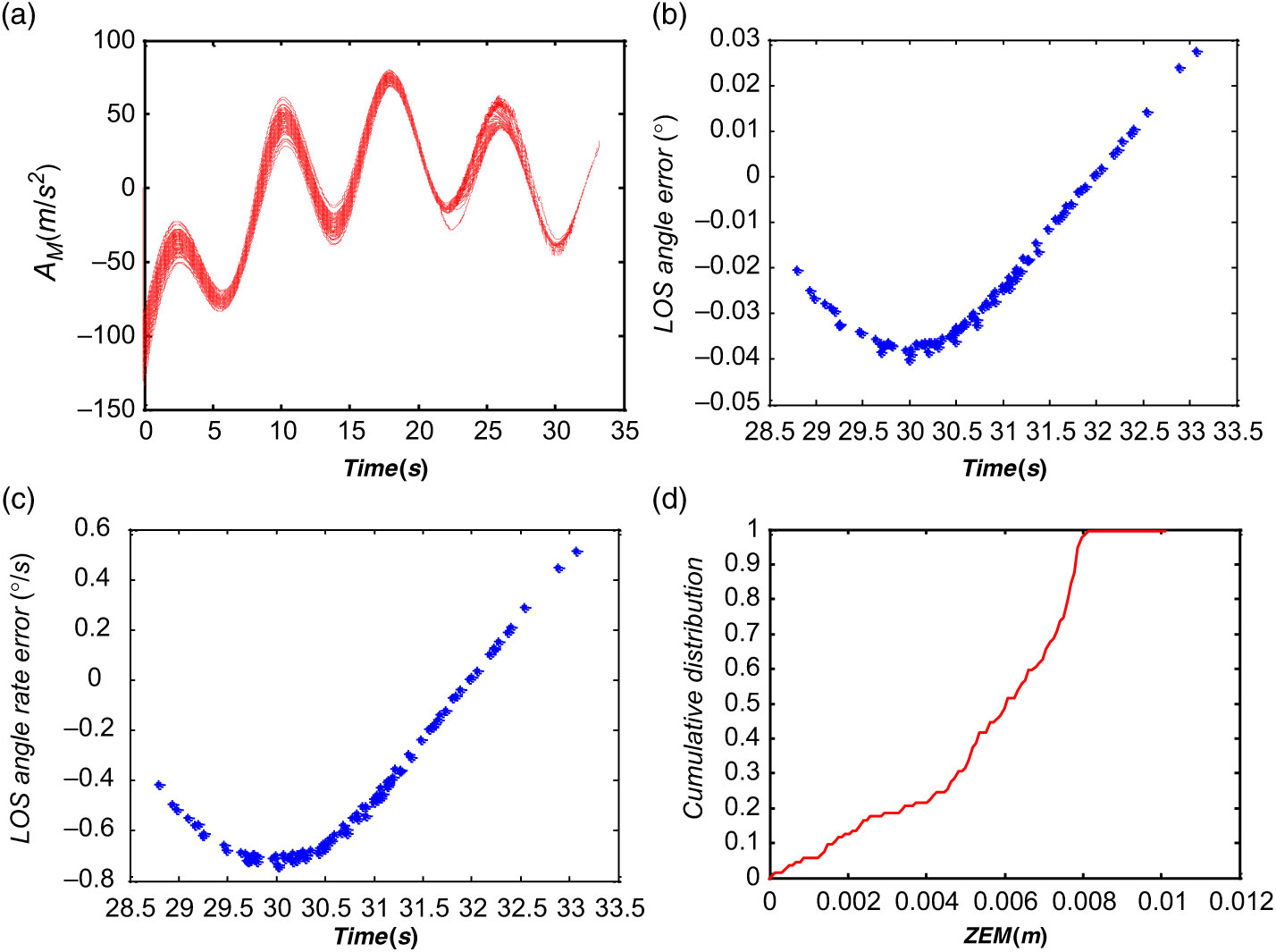
Figure 4. Monte Carlo results with the Hybrid guidance law: (a) Acceleration the missile achieved, (b) Scatter diagram of the terminal LOS angle error, (c) Scatter diagram of the terminal LOS angle rate error, (d) Cumulative distribution of zero-effort miss.