2.0 FORCES AND MOMENTS DUE TO MULTIPLE CONTROL SURFACES

The forces and moments along the three axis are denoted (1b) by C_α with the index α running (1a) from one to six:

(1a,b) $$\alpha = 1,2, \ldots ,6:\quad \quad \quad \quad \quad \quad \quad {C_\alpha } = \left\{ {X,Y,Z,L,M,N} \right\};$$

the index i numbers the N control surfaces.

(2a,b) $$i = 1, \ldots ,N = 5:\quad i = \left\{ {{\rm{body}}\;{\rm{flap,}}\;{\rm{inner}}\;{\rm{flap,}}\;{\rm{middle}}\;{\rm{flap,}}\;{\rm{outer}}\;{\rm{flap,}}\;{\rm{rudder}}} \right\}.$$

The forces and moments due to the deflection δ_i of a surface are assumed to: (a) depend only on the deflection of that surface; (b) to be specified by a polynomial of the second degree:

(3) $${C_\alpha }\left( {{\delta _i}} \right) = {C_{\alpha 0}} + {a_{\alpha i}}{\delta _i} + {b_{\alpha i}}{\left( {{\delta _i}} \right)^2},$$

(4a-c) $${C_{\alpha 0}} = {C_\alpha }\left( {{\delta _i} = 0} \right),{a_{\alpha i}} = {{d{C_{\alpha i}}} \over {d{\delta _i}}},2{b_{\alpha i}} = {{{d^2}{C_{\alpha i}}} \over {d\delta _i^2}},$$

which involves: (i) the static coefficient (4a); (ii) the control slope (4b); (iii) the control curvature (4c). The assumptions (a) and (b) do not restrict the subsequent applications in this paper, and the generalisation of the theory to remove these two restrictions is omitted for reasons of brevity. The presentation of the method of maximisation of control power is thus made under the assumptions (a) and (b). The control effect for the surface i is the deviation from the static value:

(5) $$\Delta {C_{\alpha i}}\left( {{\delta _i}} \right) = {C_{\alpha i}}\left( {{\delta _i}} \right) - {C_{\alpha 0}} = {a_{\alpha i}}{\delta _i} + {b_{\alpha i}}{\left( {{\delta _i}} \right)^2}.$$

The sum over all control surfaces of (3)/(5) specifies:

(6) $${C_\alpha } = \sum\limits_{i = 1}^N {C_{\alpha i}} = {\kern 1pt} {C_{\alpha 0}} + \sum\limits_{i = 1}^N \left[ {{a_{\alpha i}}{\delta _i} + {b_{\alpha i}}{{\left( {{\delta _i}} \right)}^2}} \right],$$

(7) $$\Delta {C_\alpha } = \sum\limits_{i = 1}^N \Delta {C_{\alpha i}} = \sum\limits_{i = 1}^N \left[ {{a_{\alpha i}}{\delta _i} + {b_{\alpha i}}{{\left( {{\delta _i}} \right)}^2}} \right],$$

the total force/moment (6) and the total control effect (7).

3.0 EXTREMA (MAXIMUM AND MINIMUM) OF FORCES AND MOMENTS

The extremum of a force or moment is obtained for the deflection which leads to a zero derivative (8a):

(8a,b) $$0 = {{d{C_{\alpha i}}} \over {d{\delta _i}}} = {a_{\alpha i}} + 2{b_{\alpha i}}{\kern 1pt} {\bar \delta _i},\quad {\bar \delta _i} = - {{{a_{\alpha i}}} \over {2{b_{\alpha i}}}}.$$

In the case of quadratic control polynomial (3) there is only one extremum (8b). If the second-order derivative is positive/negative the extremum is a minimum/maximum:

(9a,b) $${{{d^2}{C_{\alpha i}}} \over {d\delta _i^2}} = 2{b_{\alpha i}} = \left\{ {\matrix{ { > 0} & {{\rm{implies}}\;{{\bar \delta }_i}\;{\rm{is}}\;{\rm{minimum}}\;{\rm{of}}\;{C_{\alpha i}}{\rm{,}}\;\;} \cr { < 0} & {{\rm{implies}}\;{{\bar \delta }_i}\;{\rm{is}}\;{\rm{maximum}}\;{\rm{of}}\;{C_{\alpha i}}{\rm{.}}\;\;} \cr } } \right.$$

The value of the extremum is:

(10) $${\bar C_{\alpha i}} = {C_{\alpha i}}\left( {{{\bar \delta }_i}} \right) = {C_{\alpha 0}} + {a_{\alpha i}}{\bar \delta _i} + {b_{\alpha i}}{\left( {{{\bar \delta }_i}} \right)^2} = {C_{\alpha 0}} + {a_{\alpha i}}\left( { - {{{a_{\alpha i}}} \over {2{b_{\alpha i}}}}} \right) + {b_{\alpha i}}{\left( { - {{{a_{\alpha i}}} \over {2{b_{\alpha i}}}}} \right)^2},$$

which simplifies to (11b):

(11a,b) $${\delta _{{i_{\min }}}} \le {\bar \delta _i} \le {\delta _{{i_{\max }}}}:{\bar C_{\alpha i}} \equiv {C_{\alpha 0}} - {{{{\left( {{a_{\alpha i}}} \right)}^2}} \over {4{\kern 1pt} {b_{\alpha i}}}}.$$

This extremum (11b) is achievable only if the value (8b) lies within the limits of deflection of the control surface (11a). If not, then the extremum lies at one of the deflection limits, as detailed next.

4.0 EXTREMA IN THE DEFLECTION RANGE OR AT THE LIMITS

Consider first that a maximum of C _αi is sought. It will occur in the range of deflection if (9b,11a) are met:

(12a-c) $${\delta _{{i_{\min }}}} \le {\bar \delta _i} = - {{{a_{\alpha i}}} \over {2{b_{\alpha i}}}} \le {\delta _{{i_{\max }}}};{\kern 1pt} {\kern 1pt} {\kern 1pt} {\kern 1pt} {\kern 1pt} {b_{\alpha i}} < 0:{\kern 1pt} {\kern 1pt} {\kern 1pt} {\kern 1pt} {\kern 1pt} {\kern 1pt} {\kern 1pt} {\kern 1pt} {\kern 1pt} {C_{\alpha {i_{\max }}}} = {C_{\alpha i}}\left( {{{\bar \delta }_i}} \right) = {C_{\alpha 0}} - {{{{\left( {{a_{\alpha i}}} \right)}^2}} \over {4{b_{\alpha i}}}},$$

if (12a) is not met the maximum (12c) is not achievable, because it lies outside the deflection range; if (12b) is not met there is no maximum, and there is a minimum instead (9a). In both cases the maximum will be at one of the extreme deflections. If the extreme defections are symmetric (13a):

(13a,b) $${\delta _{{i_{\min }}}} = - {\delta _{{i_{\max }}}}:{\kern 1pt} {C_{\alpha {i_{\max }}}} = \left\{ {\matrix{ {{C_{\alpha i}}\left( {{\delta _{{i_{\max }}}}} \right)} & {{\rm{if}}\;\quad {a_{\alpha i}}{\kern 1pt} {\rm{ > }}{\kern 1pt} {\rm{0}},\;\;} \cr {{C_{\alpha i}}\left( {{\delta _{{i_{\min }}}}} \right)} & {{\rm{if}}\;\quad {a_{\alpha i}}{\kern 1pt} {\rm{ < }}{\kern 1pt} {\rm{0}},\;\;} \cr } } \right.$$

the maximum will be at: (i) the largest deflection (13a) for positive slope; (ii) the lowest deflection (13b) for negative slope. The reason is that symmetric deflection (14a) implies (14b).

(14a,b) $${\delta _{{i_{\min }}}} = - {\delta _{{i_{\max }}}}:{b_{\alpha i}}{\left( {{\delta _{{i_{\min }}}}} \right)^2} = {b_{\alpha i}}{\left( {{\delta _{{i_{\max }}}}} \right)^2},$$

and thus:

(15) $${C_{\alpha i}}\left( {{\delta _{{i_{\max }}}}} \right) - {C_{\alpha i}}\left( {{\delta _{{i_{\min }}}}} \right) = {a_{\alpha i}}\left( {{\delta _{{i_{\max }}}} - {\delta _{{i_{\min }}}}} \right).$$

Thus the maximum is at ${\delta _{{i_{\max }}}}$ if ${a_{\alpha i}} > 0$ and at ${\delta _{{i_{\min }}}}$ if ${a_{\alpha i}} < 0$ .

In the case a minimum is sought similar reasonings apply. The minimum lies within the range of deflection if (9a)=(16b) and (11a)=(16a) are met, and then takes the value (11b)=(16c):

(16a-c) $${\delta _{{i_{\min }}}} \le {\bar \delta _i} = - {a_{\alpha i}}/2{b_{\alpha i}} < {\delta _{{i_{\max }}}},{\kern 1pt} {\kern 1pt} {\kern 1pt} {\kern 1pt} {b_{\alpha i}} > 0:\quad {C_{\alpha {i_{\min }}}} = {C_{\alpha i}}\left( {{{\bar \delta }_i}} \right) = {C_{\alpha 0}} - {\left( {{a_{\alpha i}}} \right)^2}/4{b_{\alpha i}}.$$

If one of the conditions (16a,b) is not met, the minimum is at an extreme of the range of deflection. In the case of symmetric maximum deflections the minimum is: (i) at the lowest deflection (17a) for positive slope; (ii) at the largest deflection (17b) for negative slope:

Table 1 Reference flight condition

(17a,b) $${\delta _{{i_{\min }}}} = - {\delta _{{i_{\max }}}}:{C_{\alpha {i_{\min }}}} = \left\{ {\matrix{ {{C_{\alpha i}}\left( {{\delta _{{i_{\min }}}}} \right)} & {{\rm{if}}\;\quad {a_{\alpha i}}{\kern 1pt} {\rm{ > }}{\kern 1pt} {\rm{0}},\;\;} \cr {{C_{\alpha i}}\left( {{\delta _{{i_{\max }}}}} \right)} & {{\rm{if}}\;\quad {a_{\alpha i}}{\kern 1pt} {\rm{ < }}{\kern 1pt} {\rm{0}};\;\;} \cr } } \right.$$

these conclusions follow from (15a−15c) mutatis mutandis.

5.0 REFERENCE LOW-SPEED FLIGHT CONDITION

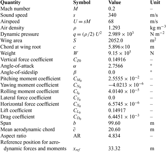
The preceding method of optimisation of control power is particularly relevant to low-speed flight for which low dynamic pressure requires larger control deflections. A straight and level steady flight at M = 0.2 is assumed, for a reference large passenger BWB whose aerodynamic and control data indicated in the Tables 1 to 3. The data in Table 1 leads to a lift coefficient that balances the weight:

(18a) $${C_{L0}} = 2W/\rho S{V^2} = W/qS = 0.14916.$$

The static lift coefficient is given in Table 2 for zero side-slip angle:

(18b) $$\beta = 0:\quad \quad \quad \quad \quad \quad {C_{L0}} = - {\kern 1pt} 0.0117 + 3.3516\alpha - 0.16966{\alpha ^2}.$$

For the value (18a) of the lift coefficient (18b) the angle-of-attack is a root of (19a):

Table 2 Static force and moment coefficients $${C_\alpha } = {c_{\alpha 0}} + {a_{\alpha 1}}{\kern 1pt} \alpha + {b_{\alpha 2}}{\kern 1pt} {\alpha ^2}$$ at β = 0

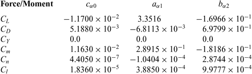
Table 3 Flap force and moment coefficients

(19a,b) $${\alpha ^2} - 19.7548\alpha + 0.94813 = 0;\quad \quad \alpha = 4.8112 \times {10^{ - 2}}{\kern 1pt} rad{ = 2.7566^ \circ },$$

the only root with a reasonable value is (19b). The value (19b) of the angle-of-attack leads to the drag (20a), side force (20b), pitching (20c), yaw (20d) and rolling (20e) moment coefficients:

(20a-e) $${C_{D0}} = 6.4760 \times {10^{ - 3}},{C_{Y0}} = 0.0,{C_{m0}} = 2.5121 \times {10^{ - 2}},$$$${C_{n0}} = - 3.8997 \times {10^{ - 6}},{C_{l0}} = 3.9361 \times {10^{ - 5}},$$

that are calculated from the formula:

(21) $${C_{\alpha 0}} \equiv {C_\alpha }\left( {{\delta _i} = 0} \right) = {c_{0\alpha }} + {a_{1\alpha }}{\kern 1pt} \alpha + {b_{2\alpha }}{\kern 1pt} {\alpha ^2},$$

using the static coefficients in Table 2.

The horizontal and vertical force coefficients in body axis are specified by the lift and drag coefficients (Fig. 1) by:

(22a,b) $$\left[ {\matrix{ {{C_{Z0}}} \cr {{C_{X0}}} \cr } } \right] = \left[ {\matrix{ {\cos \alpha } & {\sin \alpha } \cr { - \sin \alpha } & {\cos \alpha } \cr } } \right]\left[ {\matrix{ {{C_{L0}}} \cr {{C_{D0}}} \cr } } \right] = \left[ {\matrix{ {1.4930 \times {{10}^{ - 1}}} \cr { - {\kern 1pt} 7.0507 \times {{10}^{ - 4}}} \cr } } \right].$$

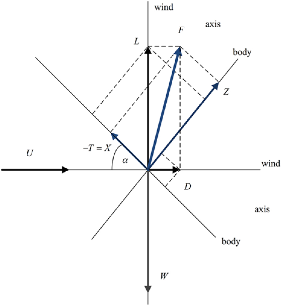
Figure 1: Relations between lift L and drag D in wind axis and longitudinal X and transverse Z forces in body axis.

The lift coefficient (18a) and the vertical force coefficient (22a) are close because the angle-of-attack is small; the horizontal force coefficient (22b) is much smaller than the drag coefficient (20c) and with opposite sign. The pitch trim is considered with: (i) the weight applied at the c.g. at quarter chord (23a); (ii) the pitching moment, as all other aerodynamic forces at the reference point (23b); (iii) relative distance is (23c):

(23a-c) $${x_{cg}} = 0.25{\kern 1pt} c = 14.74m,\;{x_{ref}} = 0.565{\kern 1pt} c = 33.31m,$$$$\bar x = {x_{ref}} - {x_{cg}} = 0.315{\kern 1pt} c = 18.57{\kern 1pt} m.$$

The balance of pitching moment for lift equal to weight (24a) is (24b):

(24a-c) $$L = W:M = {M_0} - W{\kern 1pt} \bar x,{C_m} = {C_{m0}} - 2W\bar x/\rho S{U^2}\ell \equiv {C_{m0}} + \Delta {C_m},$$

corresponding to (24c) the reference length is (25a). It leads to the pitching moment coefficient (25b):

(25a,b) $$\ell = 36.416m;\Delta {C_m} = - 2W{\kern 1pt} \bar x/\rho S{U^2}\ell = - 7.6064 \times {10^{ - 2}},$$

using also the values from Table 1. From (20c) and (25b) it follows that the pitching moment coefficient to be trimmed is

(26) $${C_m} = {C_{m0}} + \Delta {C_m} = - 5.0943 \times {10^{ - 2}},$$

that is a pitch down.

6.0 PITCH TRIM WITH MINIMUM DRAG

The pitching moment coefficient (25b) must be balanced by deflection of the control surfaces:

(27) $$ - {\kern 1pt} 7.6064 \times {10^{ - 2}} = \sum\limits_{i = 1}^5 {a_{Mi}}{\delta _i} + {b_{Mi}}\delta _i^2,$$

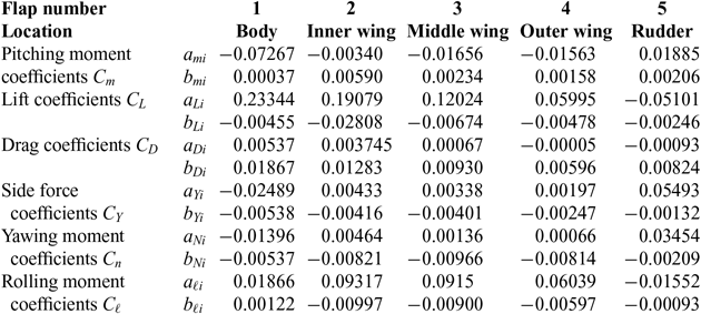
where δ_i is the deflection of each flap, and all flap coefficients a_αi and b_αi are listed in Table 3; they were calculated from tables for zero angle-of-sideslip (β = 0) and angles-of-attack α = 4^° and α = 6^°, interpolating linearly for the angle-of-attack (19b). These interpolated polynomial coefficients are then used to calculate forces and moments coefficients, e.g. the pitching moment (27) for the exact angle-of-attack (19b). The (i) linear interpolation of force and moment coefficients would have given an error O(α)² equivalent to neglecting the second-order term; the (ii) interpolation of the polynomial coefficients should give in the force and moment with an error O(α)³, consistent with retaining the second-order term and omitting the third-order term. The former (i) would represent a degradation in accuracy whereas the latter (ii) does not, and hence is adopted in the present calculation. The trimming should not change the lift (28a)

(28a,b) $$0 = \sum\limits_{i = 1}^5 \left( {{a_{Li}}{\delta _i} + {b_{Li}}\delta _i^2} \right),\quad {\kern 1pt} {\kern 1pt} {\kern 1pt} {\kern 1pt} {\kern 1pt} {\kern 1pt} {\kern 1pt} {\kern 1pt} {\kern 1pt} {\kern 1pt} {\kern 1pt} {\left( {{C_D}} \right)_{\min }} = \sum\limits_{i = 1}^5 \left( {{a_{Di}}{\delta _i} + {b_{Di}}\delta _i^2} \right),$$

and should minimise the drag (28b). The choice of minimisation drag while keeping lift and pitch trim is intended to avoid flight path changes that can be dangerous in low-speed flight near the ground. Using the values in Table 3, the optimisation problem is: (i) to keep constant the lift (29) and pitching moment (30):

(29) $$0 = {\kern 1pt} \Delta {C_L} = 0.23344{\delta _1} - 0.00455{\left( {{\delta _1}} \right)^2} + 0.19079{\delta _2} - 0.02808{\left( {{\delta _2}} \right)^2} + 0.12024{\delta _3}$$$$ - 0.00674{\left( {{\delta _3}} \right)^2} + 0.05995{\delta _4} - 0.00478{\left( {{\delta _4}} \right)^2} - 0.05101{\delta _5} - 0.00246{\left( {{\delta _5}} \right)^2};$$

(30) $${C_m} = 2.5121 \times {10^{ - 2}} - 0.07267{\delta _1} + 0.00037{\left( {{\delta _1}} \right)^2} - 0.00340{\delta _2} + 0.00590{\left( {{\delta _2}} \right)^2} - 0.01656{\delta _3}$$$$\quad + 0.00234{\left( {{\delta _3}} \right)^2} - 0.01563{\delta _4} + 0.00158{\left( {{\delta _4}} \right)^2} + 0.01885{\delta _5} + 0.00206{\left( {{\delta _5}} \right)^2};$$

(31) $${\left( {\Delta {C_D}} \right)_{\min }} = 0.00537{\delta _1} + 0.01867{\left( {{\delta _1}} \right)^2} + 0.003745{\delta _2} + 0.01283{\left( {{\delta _2}} \right)^2} + 0.00067{\delta _3}$$$$\quad + 0.00930{\left( {{\delta _3}} \right)^2} - 0.00005{\delta _4} + 0.00596{\left( {{\delta _4}} \right)^2} - 0.00093{\delta _5} + 0.00824{\left( {{\delta _5}} \right)^2}.$$

(ii) to minimise the drag (31). Eight methods of optimisation with constraints were presented in an earlier paper^{(Reference Campos and Marques6)}; of these, method VIII offered the best combination of accuracy, simplicity and clarity of interpretation. It is based on selecting the most effective control surfaces to generate each component of the aerodynamic force or moment of interest. This method is used in the sequel with suitable adaptations.

For a first iteration only terms linear in the deflections are considered. Concerning the drag it is reduced (Table 3) by: (i) negative deflection of the first three flaps, with the body flap being most effective; (ii) positive deflection or the outer flap and rudder, with the rudder being most effective. As concerns drag control the least effective surfaces are the middle and outer flaps; thus the optimisation is performed most accurately if the deflections δ ₄ and δ ₃ are eliminated from the system of equations (29–31), as follows: (i) the linear form of (29) is used to express approximately the deflection of the outer wing flap in terms of the others:

(32) $${\delta _4} = - {\kern 1pt} 3.8939{\delta _1} - 3.1825{\delta _2} - 2.0057{\delta _3} + 0.8509{\delta _5};$$

(ii) this is substituted in the remaining constraint, i.e. constant pitching moment (30; 26), and the objective, i.e. minimum drag (31), which became independent of δ ₄:

(33a) $$ - {\kern 1pt} 7.6064 \times {10^{ - 2}} = - 0.01181{\delta _1} + 0.04634{\delta _2} + 0.01479{\delta _3} + 0.005550{\delta _5},$$

(33b) $$\Delta {C_D} = 0.005565{\delta _1} + 0.003904{\delta _2} + 0.0007703{\delta _3} - 0.0009725{\delta _5};$$

(iii) the deflection δ ₃ of the next least effective control surface is expressed in terms of the remaining more effective using the second constraint (33a) of constant pitching moment:

(34) $${\delta _3} = - {\kern 1pt} 5.1429 + 0.7985{\delta _1} - 3.1332{\delta _2} - 0.3753{\delta _5};$$

(iv) substituting (34) into (33b) specifies the drag, satisfying both constraints on lift and pitching moment, in terms of the deflections of the three most effective control surfaces:

(35) $$\Delta {C_D} = - {\kern 1pt} 0.003969 + 0.006180{\delta _1} + 0.001490{\delta _2} - 0.001262{\delta _5};$$

(v) the quadratic terms are re-introduced in the drag in the same proportion to the linear terms as before in (31):

(36) $$\Delta {C_D} = - {\kern 1pt} 0.0003969 + 0.006180{\delta _1}\left( {1 + 3.4767{\delta _1}} \right)$$$$\quad + 0.001490{\delta _2}\left( {1 + {\kern 1pt} 3.4259{\delta _2}} \right) - 0.001262{\delta _5}\left( {1 - 8.8602{\delta _5}} \right),$$

leaving a formula for minimisation without constraints, with three independent variables.

The next steps are: (vi) the deflections of the body δ ₁ and inner δ ₂ flaps must be negative to minimise the drag, whereas the deflection of the rudder must be positive to further reduce drag, as follows from (8b):

(37a) $${\bar \delta _1} = - {\kern 1pt} 1/\left( {2 \times 3.4767} \right) = - 0.14381{\kern 1pt} rad = - {8.2399^ \circ },$$

(37b) $${\bar \delta _2} = - {\kern 1pt} 1/\left( {2 \times 3.4259} \right) = - 0.14595{\kern 1pt} rad = - {\kern 1pt} {8.3621^ \circ },$$

(37c) $${\bar \delta _5} = 1/\left( {2 \times 8.8602} \right) = 0.056432{\kern 1pt} rad{ = 3.2333^ \circ };$$

(vii) the substitution of (37a–c) in (34) and (32) would lead to the deflection of the two least effective surfaces,

(37d,e) $${\bar \delta _3} = - {\kern 1pt} 4.8216{\kern 1pt} rad = - {\kern 1pt} {276.26^ \circ },\quad {\bar \delta _4} = 10.325{\kern 1pt} rad = {\kern 1pt} {591.59^ \circ };$$

(viii) the values (37d,e) exceed the limit δ ₀ = 25^°; (ix) since these are the least effective control surfaces, the values (37d,e) are discarded, viz. these surface are not used δ ₃ = 0 = δ ₄, so the deflections are:

(38) $${\bar \delta _i} = \left( { - {\kern 1pt} 0.14381, - {\kern 1pt} 0.14595,0,0, + 0.056432} \right){\kern 1pt} rad = {\left( { - {\kern 1pt} 8.2399, - {\kern 1pt} 8.362,10,0, + 3.2333} \right)^ \circ };$$

(viii) the corresponding drag (31)is(39a):

(39a,b) $${\left( {\Delta {C_D}} \right)_{\min }} \equiv \Delta {\bar C_D} = \Delta {C_D}\left( {{{\bar \delta }_i}} \right) = - 6.8567 \times {10^{ - 4}},\quad \quad \quad {\left( {\Delta {C_D}} \right)_{\min }}/{C_{D0}} = - 0.10588,$$

and thus the pitch trim decreases drag (20a) by 10.6% in (39b) to the value:

(39c) $${C_{D\min }} = {C_{D0}} + {\left( {\Delta {C_D}} \right)_{\min }} = 6.4760 \times {10^{ - 3}} - 5.7903 \times {10^{ - 4}} = 5.7903 \times {10^{ - 3}},$$

(x) the comparison with pitch trim by the body flap alone (40a) i.e. the first term of (30) with unchanged C_m leads (40b) to a large deflection (40c), close to the limit ±25^°:

(40a-d) $${\bar {\bar \delta}} _{2} = {\bar {\bar \delta}} _{3} = {\bar {\bar \delta}} _{4} = {\bar {\bar \delta}} _{5} = 0:\quad {\left( {{{\bar {\bar \delta}} }_{1}} \right)^2} - 196.41{\bar {\bar \delta}} _{1} + 67.895 = 0,\quad {\bar {\bar \delta}} _{1} = - 0.{\kern 1pt} 34633{\kern 1pt} rad = - {\kern 1pt} {19.84^ \circ };$$

(xi) the associated drag would be a penalty (40e) instead of a reduction for the optimal solution (39b), that is as increase (40f) of 63.3% instead of a reduction (39b) of 10.6%:

(40e,f) $$\Delta {\bar {\bar C}}_{D} = \Delta {C_D} ( {{{\bar {\bar \delta}}}_{i}} ) = 0.00537{\bar {\bar \delta}} _{1} + 0.01867{( {{{\bar {\bar \delta}} _{1}} )^2} = 4.098 \times {10^{ - 3}},\Delta {\bar {\bar C}}_D}/{C_{D0}} = 0.63286.$$

(xii) full pitch trim (30) with (26) would require (40g) a deflection of the body flap (40h) not possible within the 25^o limit:

(40g,h) $${\left( {{{\tilde \delta }_1}} \right)^2} - 196.41{\tilde \delta _1} + 205.58 = 0,\quad {\tilde \delta _1} = 1.0523{\kern 1pt} rad{ = 60.294^ \circ }{ > 25^ \circ }.$$

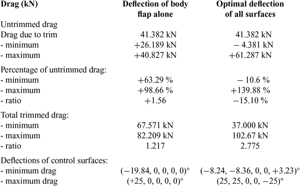
In conclusion A1 the optimal pitch trim (38) compared with deflection of body flap alone (40a,c) gives: (a) smaller deflections of control surfaces (38)vs. (40d); (b) lower trim drag (39a)vs. (40e) by a difference (41a) that corresponds (41b) to 73.9% of the drag;

(41a,b) $$\Delta {\bar C_D} - \Delta {\bar {\bar C}}_{D} = - 4.7837 \times {10^{ - 3}},\quad \quad \quad \left( {\Delta {{\bar C}_D} - \Delta {{\bar {\bar C}}_{D}}} \right)/{C_{D0}} = 0.73868;$$

(c) a trim drag reduction of 10.6% in (39b) the optimal case vs. a drag penalty of 63.3% in (40f) using the body flap alone; (d) in the comparison (a–c) it is assumed (26) constant, since full pitch trim is not possible (40g,h) with body flap alone.

7.0 MAXIMUM DRAG FOR GREATEST RETARDATION

The minimum drag for pitch trim is desirable for the fastest climb after take-off; the reverse, the maximum drag with pitch trim, may be desirable for the steepest descent to land. The preceding analysis applies because in both cases lift balance and pitch trim must be maintained, and the most effective control surfaces should be used, leading to the total drag (36) without constraint. Maintaining lift and pitch trim avoids flight path corrections, which may be a risk in low-speed flight near the ground, due to control surface and/or engine throttle delays. The only difference is that (36) should be maximised rather than minimised: (i) since (δ ₁, δ ₂) lead to a minimum (37a, 37b), the maximum is at maximum positive deflection, taken to be 25^° in

Table 4 Effect of pitch trim on drag

(42a,b); (ii) conversely the maximum drag for δ ₅ is at the smallest deflection in (42c):

(42a-c) $$\left\{ {{{\tilde \delta }_1},{{\tilde \delta }_2},{{\tilde \delta }_3},{{\tilde \delta }_4},{{\tilde \delta }_5}} \right\} = \left\{ {{{25}^ \circ }{{,25}^ \circ },0,0, - {{25}^ \circ }} \right\} = 0.43633rad\left\{ {1,1,0,0, - 1} \right\} \equiv \left\{ {{\delta _0},{\delta _0},0,0, - {\delta _0}} \right\};$$

(iii) the two least effective control surfaces are not used in the drag difference (36) leading to (43):

(43) $${\left( {\Delta {C_D}} \right)_{\max }} = - 0.0003969 + 0.006408{\delta _0} + 0.03777\delta _0^2 = 9.5909 \times {10^{ - 3}};$$

(iv) the maximum extra drag (43) with a limit of 25^° on deflection is (44a) more than the baseline drag (20a):

(44a,b) $${\left( {\Delta {C_D}} \right)_{\max }}/{C_{D0}} = 1.481,\quad {\left( {\Delta {C_D}} \right)_{\max }}/{\left( {\Delta {C_D}} \right)_{\min }} = 13.988,$$

and is over 13 times (44b) the minimum drag (39a) for pitch trim; (v) thus the maximum trimmed drag is more than twice the untrimmed drag (45):

(45) $$0.89412 \le {C_{D\min }}/{C_{D0}} \le {C_D}/{C_{D0}} \le {C_{D\max }}/{C_{D0}} \le 2.481 \equiv k;$$

(vi) this shows the range of possible trimmed drag coefficients:

(46) $$5.7903 \times {10^{ - 3}} \le {C_{D\min }} \le {C_D} \le {C_{D\max }} \le 1.6067 \times {10^{ - 2}}.$$

In conclusion (Table 4), there is a wide range of trimmed drag variations obtained by optimizing control surface deflections, from a reduction of 10.6% in (39b) to an increase of 139.9% in (44a). If the body flap alone had been used at maximum deflection (47a) the drag increase (36) would be smaller (47b):

(47a-c) $${\tilde {\tilde \delta}} _{1} = {25^ \circ };{\tilde {\tilde \delta} _{5}} = {\tilde {\tilde \delta} _{2}} = 0:\Delta {\tilde {\tilde C}_{D}} = \Delta {C_D}( {{{\tilde {\tilde \delta }_i}}}) = 6.3892 \times {10^{ - 3}},\Delta {{\tilde {\tilde C}_{D}}} \mathord{/ {\vphantom {{\Delta {{\tilde {\tilde C}_{D}} {{C_{D0}} = 0.9866,}}} . } {{C_{D0}} = 0.9866,}}} $$

viz. 98.7% in (47b) instead of 139.9% in (44a). Thus maximum deflection of the body flap alone would have less than doubled the trim drag (47a), whereas optimal deflections more than doubles it (44a). The range of drag modulation using optimal controls is much larger than using body flap alone because: (i) the minimum trimmed drag is smaller (48a) and the maximum trimmed drag is larger (48b):

(48a-c) $${k_1} \equiv \Delta {\bar {\bar C}}_{D}/{\left( {\Delta {C_D}} \right)_{\min }} = - 9.3181;{k_2} \equiv {\left( {\Delta {C_D}} \right)_{\max }}/\Delta {\bar {\bar C}}_{D} = 1.501;{k_1}{\kern 1pt} {k_2} = - 13.988;$$

(ii) the product (48c) ≡(44b) shows that the range of drag modulation with optimal controls is more than 13 times larger than with body flap alone. This demonstrates the contrast between: (a) choosing “à priori” single control surface, even the most effective (body flap), which requires a large deflection (40d) for constant (26) with minimum drag, and would became saturated for not much larger drag, giving a small range of drag modulation and cannot provide full bitch trim (40g, h), (b) usingoptimal deflections of all control surfaces, which allows pitch trim with a drag reduction (39b), and can also lead to a large drag increase (44a), providing a wide range of drag modulation (46). A wide range of drag is useful for steep descent allowing a continuous adaptation of the trajectory. The results on the range of possible drag modulation with pitch trim are compared in the Table 4 using total drag or thrust instead of drag coefficient by multiplying by:

(49) $$D/{C_D} = {1 \over 2}{\kern 1pt} \rho S{U^2} = 6.1343 \times {10^6}{\kern 1pt} N.$$

It demonstrates the superiority of pitch control by optimal deflection of all surfaces versus body flap alone.

8.0 MAXIMUM AND MINIMUM ACHIEVABLE PITCHING MOMENT

The maximum and minimum pitching moment (section 8) determines the extremes of the c.g. range, which can be trimmed for several possible engine positions in the vertical plane relative to the aircraft datum. The aim next is to find the maximum and minimum of the pitching moment (50a) keeping constant the lift (18a) ≡ (50b) and drag (20a) ≡ (50c) coefficients (50b,c):

(50a,c) $${C_{m{\kern 1pt} {\kern 1pt} \max ,\min }}:\quad \quad {C_L} = {C_{L0}} = 0.14916,\quad \quad {C_D} = {C_{D0}} = 6.4760 \times {10^{ - 3}}.$$

The Table 3 shows that the least effective control surfaces for the pitching moment (30) are the inner δ ₂ and outer δ ₄ wing flaps; thus these are eliminated using the constraints. The sequence of steps is as follows: (i) the deflection δ ₂ of the least effective control surface is expressed in terms of all the other deflections from the condition (50b) of constant lift in the linearised form of (29):

(51) $${\delta _2} = - {\kern 1pt} 1.22350{\delta _1} - {\kern 1pt} 0.63022{\delta _3} - 0.31422{\delta _4} + 0.26736{\delta _5};$$

(ii) substitution of the condition (51) of constant lift in the drag (31; 39a) and in the pitching moment (30), eliminates the deflections δ ₂, and leaves the remaining deflections:

(52a) $$ - 6.8567 \times {10^{ - 4}} = 0.00078799{\delta _1} - 0.0016902{\delta _3} - 0.0012268{\delta _4} + 0.000071039{\delta _5},$$

(52b) $${C_m} = 0.025121 - 0.068510{\delta _1} - 0.014417{\delta _3} - 0.014562{\delta _4} + 0.017941{\delta _5};$$

(iii) the condition of constant drag (52a) is used to express the deflection δ ₄ of the second least effective pitch control surface in terms of the remaining deflections.

(53) $${\delta _4} = 0.55891 + 0.64224{\delta _1} - 1.3777{\delta _3} + 0.0057874{\delta _5};$$

(iv) substitution of (53) in (52b) eliminates the deflection of the two least effective control surfaces:

(54) $${C_m} = 0.016982 - 0.077862{\delta _1} + 0.0056451{\delta _3} + 0.017857{\delta _5},$$

from the pitching moment (54), which is thus unconstrained.

Next (v) the non-linear terms in the pitching moment are restored in the same proportion as in (30), leading to:

(55) $${C_m} = 0.016962 - 0.077862{\delta _1}\left( {1 - 0.0050915{\delta _1}} \right) \quad \\ - 0.0056451{\delta _4}\left( {1 - 0.10109{\delta _4}} \right) + 0.017857{\delta _5}\left( {1 + 0.10928{\delta _5}} \right);$$

(vi) the extrema of the pitching moment relative to the three most effective pitch control surfaces (with the other two implicitly included through the constraints) are minima at the deflections (8b), leading to the values:

(56) $$\left\{ {{{\bar \delta }_1},{{\bar \delta }_3},{{\bar \delta }_5}} \right\} = \left\{ {98.203,4.9461, - {\kern 1pt} 4.5754} \right\};$$

(vii) these values (56) are far outside the range of possible deflections (57a):

(57a-c) $$\left| {{\delta _i}} \right| \le {25^ \circ } = 0.43633{\kern 1pt} rad = {\delta _0};{\delta _0} = - {\kern 1pt} {\hat \delta _1} = - {\kern 1pt} {\hat \delta _4} = {\hat \delta _5};{\delta _0} = {\mathord{\buildrel{\lower3pt\hbox{$\scriptscriptstyle\smile$}}\over \delta } _1} = {\mathord{\buildrel{\lower3pt\hbox{$\scriptscriptstyle\smile$}}\over \delta } _4} = - {\mathord{\buildrel{\lower3pt\hbox{$\scriptscriptstyle\smile$}}\over \delta } _5},$$

thus the maximum (minimum) pitching moment occur respectively for the deflections (57b) and (57c); (viii) these correspond to:

(58a,b) $${\left( {{C_m}} \right)_{\max }} = {C_m}\left( {{{\hat \delta }_{\hat i}}} \right) = 6.2462 \times {10^{ - 2}},{\left( {{C_m}} \right)_{\min }} = {C_m}\left( {{{\mathord{\buildrel{\lower3pt\hbox{$\scriptscriptstyle\smile$}}\over \delta } }_i}} \right) = - 2.5992 \times {10^{ - 2}},$$

the maximum (58a) and minimum (58b) pitching moment.

9.0 MAXIMUM AND MINIMUM ACHIEVABLE YAWING MOMENT

The engine position relative to the horizontal datum and the maximum and minimum pitching moment (section 8) determine the trimmable c.g. range. The compensation of an outboard engine failure (section 10) depends on the maximum and minimum yawing moment (section 9), which are calculated next. The yawing moment coefficient is given by the data in Table 3:

(59) $${C_n} = - 0.01396{\delta _1} - 0.00537{\left( {{\delta _1}} \right)^2} + 0.00464{\delta _2} - 0.00821{\left( {{\delta _2}} \right)^2} + 0.00136{\delta _3} - 0.00966{\left( {{\delta _3}} \right)^2}$$$$ + 0.00066{\delta _4} - 0.00814{\left( {{\delta _4}} \right)^2} + 0.03454{\delta _5} - 0.00209{\left( {{\delta _5}} \right)^2}.$$

The maximum and minimum are sought at constant lift (18a)≡(60a), drag (20a)≡(60b) and pitching moment (26)≡(60c).

(60a,c) $${C_{L0}} = 0.14916,\quad {C_{D0}} = 0.0064760,\quad {C_{m0}} = - 0.050943.$$

The three least effective yaw control surfaces are the outer δ ₄, middle δ ₃ and inner δ ₂ flaps; the optimal deflections of the two most effective control surfaces (δ ₁, δ ₅) follow from (8b), and are given by (68a,b). Since they exceed the limit deflection (57a), the latter is used to calculate the maximum and minimum pitching moment (69–70a,b). As a preliminary illustration their deflections will be eliminated from the yawing moment (59) using the constraints (60a–c) of constant lift, drag and pitching moment. The sequence of steps is as follows: (i) the constraint of constant lift (60a) in linearised form (29) is used to specify the deflection of the least effective yaw control surface (the outer flap) in terms of the others:

(61) $${\delta _4} = - 3.8939{\delta _1} - 3.1825{\delta _2} - 2.0057{\delta _3} + 0.85088{\delta _5};$$

(ii) the deflection of the least effective yaw control surface is eliminated from the drag (31,39a) ≡ (62a), pitching (30,25b) ≡ (62b) and yawing (59) ≡ (62c) moment:

(62a) $$ - 6.8567 \times {10^{ - 4}} = 0.0055647{\delta _1} + 0.0039041{\delta _2} + 0.0007703{\delta _3} - 0.0009729{\delta _5},$$

(62b) $$ - 0.076064 = - 0.011808{\delta _1} + 0.046343{\delta _2} + 0.014789{\delta _3} + 0.0055507{\delta _5},$$

(62c) $${C_n} = - 0.01653{\delta _1} + 0,0025396{\delta _2} + 0.000362{\delta _3} + 0.035102{\delta _5};$$

using (61).

The next step (iii) is to express the deflection δ ₃ of the second least effective yaw control surface (middle flap) in terms of the remaining deflections, e.g. using (62a):

(63) $${\delta _3} = - 0.89013 - 7.2241{\delta _1} - 5.0683{\delta _2} + 1.2630{\delta _5};$$

(iv) substitution of (63) eliminates the deflections of the two least effective yaw control surfaces from the condition of constant pitching moment (62b) and from the yawing moment (62c):

(64a) $$ - 0.0629 = - 0.11865{\delta _1} - 0.028612{\delta _2} + 0.024229{\delta _5};$$

(64b) $${C_n} = - 0.0003222 - 0.019145{\delta _1} + 0.0007049{\delta _2} + 0.035559{\delta _5};$$

(v) the deflection of the third least effective yaw control surface (inner flap) is expressed in terms of the remaining two using (64a).

(65) $${\delta _2} = 2.1984 - 4.1469{\delta _1} + 0.84681{\delta _5};$$

(vi) substitution of (65) in (64b) specifies the yawing moment in terms of the deflections of the two most effective yaw control surfaces:

(66) $${C_n} = 0.0012275 - 0.022068{\delta _1} + 0.036157{\delta _5};$$

(vii) the non-linear terms in the yawing moment (59) are restored in the same proportion to the linear terms:

(67) $${C_n} = 0.0012275 - 0.02068{\delta _1}\left( {1 + 0.38467{\delta _1}} \right) + 0.036157{\delta _5}\left( {1 - 0.06051{\delta _5}} \right);$$

(viii) the extrema are (8b) a minimum yawing moment for the deflection of the body flap (68a) and a maximum for the deflection of the rudder (68b):

(68a,b) $${\bar \delta _1} = - 1.29981,{\bar \delta _2} = 8.26316;$$

(ix) the values (68a,b) are far outside the range of possible deflections, so the maximum and minimum yawing moments are obtained:

(69a,b) $${\delta _1} = - {\delta _5}{ = 25^ \circ } = 0.43633{\kern 1pt} rad:\quad {\kern 1pt} {\kern 1pt} {\kern 1pt} {\kern 1pt} {\kern 1pt} {\kern 1pt} {\kern 1pt} {\kern 1pt} {\kern 1pt} {\kern 1pt} {\kern 1pt} \quad {\left( {{C_n}} \right)_{\min }} = - {\kern 1pt} 0.025504,$$

(69c,d) $$ - {\delta _1} = {\delta _5}{ = 25^ \circ } = 0.43633{\kern 1pt} rad:\quad {\kern 1pt} {\kern 1pt} {\kern 1pt} {\kern 1pt} {\kern 1pt} {\kern 1pt} {\kern 1pt} {\kern 1pt} {\kern 1pt} {\kern 1pt} \quad {\left( {{C_n}} \right)_{\max }} = + {\kern 1pt} 0.024096,$$

at the extreme opposite deflections of rudder and body flap.

10.0 YAW CONTROL MARGIN WITH OUTBOARD ENGINE FAILURE

The worst case scenario for yaw control is an outboard engine failure. For an aircraft with n identical engines with thrust T, and the outer engine at a distance y from the aircraft axis, the engine-out yawing moment is (70b):

(70a,b) $$D = nT:\quad {\kern 1pt} {\kern 1pt} {\kern 1pt} {\kern 1pt} {\kern 1pt} {\kern 1pt} {\kern 1pt} {\kern 1pt} {\kern 1pt} {\kern 1pt} \quad \quad \quad \quad N = yT = yD/n,$$

where the total thrust (70a) is assumed to equal the reference drag; this corresponds to the yawing moment coefficient.

(71a) $${C_n} = 2N/\left( {\rho {U^2}S\ell } \right) = \left( {y/\ell {\kern 1pt} n} \right)\left( {2D/\rho {U^2}S} \right) = {C_D}y/\ell n;$$

using the values (20a) and (25a) leads to:

(71b) $${C_n} = 2N/\left( {\rho {U^2}S\ell } \right) = \left( {y/\ell {\kern 1pt} n} \right)\left( {2D/\rho {U^2}S} \right) = \left( {{C_{D0}}{\kern 1pt} /\ell } \right)y/n = 1.7783 \times {10^{ - 4}}y/n,$$

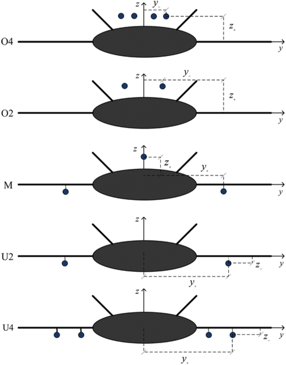
showing that the yawing moment: (i) increases with the distance of the outboard engine from the centreline; (ii) decreases with the number of engines, since for the same total drag, each engine has less thrust. A total of 5 engine configurations (Fig. 2) are considered: (i) four engines (72a) above the centre-body (O4) with failure of outboard engine at distance (72b) from centreline leads to a yawing coefficient (72c):

Figure 2: Blended wing body (BWB) with five engine configurations: (O4) four engines above the body with twin fins for noise shielding; (O2) two engines above the body; (M) one engine above the body and two un underwing nacelles; (U2) two engines in underwing nacelles; (U4) four engines in underwing nacelles.

(72a-e) $$04:n = 4,{\kern 1pt} {\kern 1pt} {\kern 1pt} {y_ - } = 8m:{C_n} = 3.5567 \times {10^{ - 4}},{C_n}/{\left( {{C_n}} \right)_{\max }} = 0.01476,$$$${C_n}/{\left( {{C_n}} \right)_{\min }} = - {\kern 1pt} 0.013946,$$

which is less than 1.5% of the maximum available yaw control power; (ii) for two engines (73a) at the same outboard position over the centre-body (O2):

(73a-e) $$02:{\kern 1pt} n = 2,{y_ - } = 8m:{C_n} = 7.1134 \times {10^{ - 4}},{C_n}/{\left( {{C_n}} \right)_{\max }} = 0.029521,{C_n}/{\left( {{C_n}} \right)_{\min }} = - {\kern 1pt} 0.02891,$$

the yawing moment is doubled, because each engine has double thrust, and less than 3.0% of the maximum yaw control power is used; (iii) for four underwing engines (U4) and failure of the outboard engine at a distance (74b) from the axis:

(74a,e) $$U4:n = 4,{\kern 1pt} {\kern 1pt} {y_ + } = 30m:{C_n} = 1.3338 \times {10^{ - 3}},{C_n}/{\left( {{C_n}} \right)_{\max }} = 0.055352,$$$${C_n}/{\left( {{C_n}} \right)_{\min }} = - 0.052296,$$

Table 5 Yaw trim compensate outboard engine failure

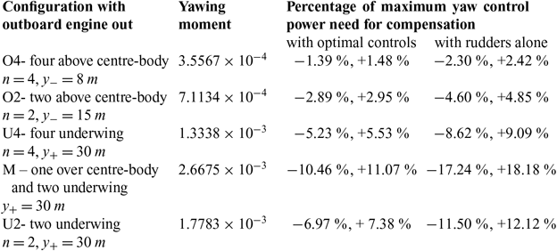
the yawing moment is less than 5.6% of the maximum available; (iv) for two underwing engines (U2) at the same outboard position:

(75a-e) $$U2:n = 2,{y_ + } = 30m:{C_n} = 2.6675 \times {10^{ - 3}},{C_n}/{\left( {{C_n}} \right)_{\max }} = 0.11070,{C_n}/{\left( {{C_n}} \right)_{\min }} = - {\kern 1pt} 0.10459,$$

the yawing moment is still less than 11 .1% of the maximum available, though this would be an extreme case of two very powerful engines far outboard; (v) for a mixed configuration (M) with one engine over the centre-body and two under the outer wings at the same distance from the axis, the yawing moment would be intermediate between the two preceding cases:

(76a,e) $$M:n = 3,{\kern 1pt} {\kern 1pt} {y_ + } = 30m:{C_n} = 1.7783 \times {10^{ - 3}},{C_n}/{\left( {{C_n}} \right)_{\max }} = 0.073802,$$$${C_n}/{\left( {{C_n}} \right)_{\min }} = - {\kern 1pt} 0.069728,$$

i.e. use less than 7.4% of the available control power. The results for the five engine configurations are summarised in Table 5.

If rudder alone had been used, then the maximum and minimum yawing coefficient would have been (59)given by:

(77) $$C_n^ \pm = \pm {\kern 1pt} 0.03454{\delta _0} - 0.00209\delta _0^2 = {\kern 1pt} \left( { + 1.4673, - 1.5469} \right) \times {10^{ - 2}};$$

the fraction of available yaw control power needed to compensate an outboard engine failure in the five cases would be:

(78a) $$O4,O2,U4,M,U2:{C_n}/C_n^ + = {\kern 1pt} {\kern 1pt} \left\{ {0.02424,0.04848,0.090902,0.1818,0.1212} \right\},$$

(78b) $${C_n}/C_n^ - = {\kern 1pt} - \left\{ {0.022992,0.045985,0.086334,0.17244,0.11496} \right\}.$$

In all cases the percentage of available yaw control power needed to compensate an out-board engine out condition is smaller for optimal controls than for rudders alone, because the yaw control authority:

(79a,b) $${\left( {{C_n}} \right)_{\max }}/C_n^ + = 1.6422,\quad {\left( {{C_n}} \right)_{\max }}/C_n^ - = 1.4248,$$

is increased by a factor of about 1.5 by the use of optimal controls, and thus there is a larger safety margin to cope with other events.

11.0 MAXIMUM AND MINIMUM ROLLING MOMENT

Whereas the pitching moment (section 8) determines the c.g. range, and the yawing moment (section 9) the ability to compensate and engine out condition (section 10), the rolling moment (section 11) relates to the compensation of a vortex-wake encounter.

The rolling moment is specified by the data in Table 3:

(80) $${C_l} = 0.01866{\delta _1} + 0.00122{\left( {{\delta _1}} \right)^2} + 0.09317{\delta _2} - 0.00997{\left( {{\delta _2}} \right)^2} + 0.09150{\delta _3} - 0.00900{\left( {{\delta _3}} \right)^2}$$$$ + 0.06039{\delta _4} - 0.00597{\left( {{\delta _4}} \right)^2} - 0.01552{\delta _5} - 0.00093{\left( {{\delta _5}} \right)^2}.$$

The maximum and minimum rolling moment will be sought at constant lift, drag and pitching moment (60a-c) ≡ (81a-c) and no yawing moment (81d):

(81a,d) $${C_{L0}} = 0.14916,\quad {C_{D0}} = 0.0071036,\quad {C_{m0}} = - 0.050943,\quad {C_{n0}} = 0,$$

so that the flight path is not disturbed. The least effective roll control surfaces are the rudders (δ ₅) and the body flap (δ ₁); the outer flap (δ ₄) is less effective than the middle flap (δ ₃) and the inner flap (δ ₂) marginally more effective. The most effective control surface δ ₂ has (8b) optimal deflection (90a), which exceeds the limit (57a); the latter limit is thus taken to calculate the maximum and minimum rolling moment (90b,c). As a preliminary the deflections of the first four least effective control surfaces will be eliminated in this order using the constraints: (i) the rudder deflection δ ₅ is expressed in terms of the remaining using the condition (81d) of zero yawing moment in linearised form (59), leading to (82):

(82) $${\delta _5} = 0.40417{\delta _1} - 0.13434{\delta _2} - 0.039375{\delta _3} - 0.019108{\delta _4};$$

(ii) the deflection of the least effective roll control surface (rudder) is eliminated by replacing (82) in the conditions of constant lift (29) ≡ (83a), drag (31; 39a) ≡ (83b) and pitching moment (30, 25b) ≡ (83c):

(83a) $$0 = 0.21282{\delta _1} + 0.19764{\delta _2} + 0.12225{\delta _3} + 0.060925{\delta _4};$$

(83b) $$ - 6.8567 \times {10^{ - 4}} = 0.0049941{\delta _1} + 0.0038699{\delta _2} + 0.0007066{\delta _3} - 0.0000322{\delta _4};$$

(83c) $$ - 0.076064 = - 0.065051{\delta _1} - 0.0059323{\delta _2} - 0.017302{\delta _3} - 0.01599{\delta _4};$$

(83d) $${C_l} = 0.012387{\delta _1} + 0.095255{\delta _2} + 0.092111{\delta _3} + 0.060687{\delta _4};$$

and also in the rolling moment (80) ≡ (83d); (iii) the deflection δ ₁ of the second least effective control surface (body flap) is expressed in terms of the remaining from the lift (83a) ≡ (84):

(84) $${\delta _1} = - 0.92876{\delta _2} - 0.57448{\delta _3} - 0.28627{\delta _4};$$

(iv) substitution in the drag (83b), pitch (83c) and rolling moment (83d) coefficients eliminates the deflections of the two least effective roll control surfaces:

(85a) $$ - 6.8567 \times {10^{ - 4}} = - 0.00076833{\delta _2} - 0.0021624{\delta _3} - 0.0014618{\delta _4},$$

(85b) $$ - 0.076064 = 0.0544784{\delta _2} + 0.020068{\delta _3} + 0.0026319{\delta _4},$$

(85c) $${C_l} = 0.08375{\delta _2} + 0.084994{\delta _3} + 0.057134{\delta _4};$$

(v) the deflection δ ₄ of the third least effective roll control surface (outer flap) is expressed in terms of the remaining from the condition (85a) of constant drag:

(86) $${\delta _4} = 0.46906 - 0.52558{\delta _2} - 1.4793{\delta _3};$$

(vi) substitution of (86) leaves the deflections of the two most effective roll control surfaces in the pitching (85b) ≡ (87a) and rolling moment (85c) ≡ (87b):

(87a,b) $$ - 0.077299 = 0.053101{\delta _2} + 0.016175{\delta _3},\quad {C_l} = 0.026799 + 0.053722{\delta _2} + 0.00047567{\delta _3};$$

(vii) the deflection of the fourth least effective roll control surface (middle flap) is expressed from the pitching moment (87a)asafunction(88a) of the deflection of the most effective:

(88a,b) $${\delta _3} = - 4.7789 - 3.2829{\delta _2};\quad \quad {C_l} = 0.024526 + 0.05216{\delta _2};$$

(viii) this specifies the rolling moment in terms of (88b) the most effective roll control surface (inner flap); (ix) the non-linear terms are restored to the rolling moment coefficient (88b) in the same proportion to the linear terms as in (80) leading to (89):

(89) $${C_l} = 0.24526 + 0.05216{\delta _2}\left( {1 - 0.10701{\delta _2}} \right);$$

(xi) the extremum of (89) corresponds (8b) to a deflection (90a) far outside the range of possible values:

(90a-d) $${\bar \delta _2} = 4.6725,\quad {\bar \delta _0}{ = 60^ \circ } = 1.0472rad,{C_{l\max ,l\min }} = {C_l}\left( { \pm {\kern 1pt} {{\bar \delta }_0}{\kern 1pt} } \right) = \left( { - {\kern 1pt} 0.036217,0.073027} \right);$$

(xii) the maximum and minimum rolling moments (90b,c) thus occur at the extreme deflections, that are taken to be (90b).

12.0 CONCLUSION

The control limits of a FW configuration were explored in low-speed flight. The method used can maximise or minimise (section 3) any component of the aerodynamic forces or moments (section 2) within the range of possible deflections of each control surface (section 4); other components can be left free or constrained, e.g. by equilibrium conditions. Applying this method to a BWB in (section 5) a low-speed (M = 0.2) configuration: (i) shows that pitch trim can be obtained with a minimum drag reduction of 11%, which has beneficial effect on climb performance after take-off (section 6); (ii) conversely a maximum drag increase of 61% can be obtained with the same angle-of-attack and pitch trim for the steepest descent to land (section 7); (iii) the maximum and minimum pitching moment (section 8) using all control surfaces can be modulated over a wider range of values than using only the body flap, and similar results concern the broader range of achievable drag at constant lift with pitch trim (Table 4); (iv) the maximum and minimum yawing moment (section 9) specifies the yaw control authority available in the worst scenario of failure of an outboard engine (section 10) showing that the use of all available control surfaces is more effective than rudders alone (Table 5) leaving a greater safety margin; (v) the maximum and minimum rolling moment (section 11)also benefit from the use of all available control surfaces to achieve a broader range of values. The introduction (section 1) outlines the problem, and the conclusion (section 12) summarises the results. Some aspects of the maximisation or minimisation with constraints are discussed in the appendix. Modern “big data” methods can quickly explore many configurations to arrive at an optimum without giving much explanation about the result. The analytical methods are a good complement to numerical methods using massive computing to give a better insight on the meaning of the results, besides proving an independent check and indication of accuracy.