NOMENCLATURE
- O g x g y g z g
earth reference frame (ERF)
- Oxyz
body reference frame (BRF)
- [u, v, w]
linear velocities in BRF, m/s
- [u w , v w , w w ]
wind velocities, m/s
- V, Va
inertial speed and airspeed, m/s
- [p, q, r]
angular velocitiees in BRF, rad/s
- x g , y g , z g
Cartesian positions in ERF, m
- [ϕ,θ,ψ]
Euler attitude angles, rad
- M
mass matrix(or inertial matrix)
- x G , y G , z G
positions of gravity center, m
- x B , y B , z B
positions of buoyancy center, m
- m
total mass of the airship and payload, kg
- m 11,...,m 66
added masses, kg, kg.m or kg.m2
- I x ,...,I yz
inertial moments, kg.m2
- F GB
gravity and buoyancy force, N
- F T
thrust force, N
- F A , F w
nominal and wind-induced aerodynamic forces, N
- F I
Coriolis force, N
- B, G
gravity, buoyancy, N
- B
control allocation matrix of the propeller
- Vol
volume of the airship, m3
- L ref , Sref
reference length and reference area, m and m2
- φ, φ w
angles between the x-axis and the horizontal component of the inertial speed and airspeed respectively, rad
-
 $${\bf R}_{{\mib{I}} }^{{\mib{B}} } $$
direction cosine transformation matrix
- Φ
angular transformation matrix
- C x , C z , C my , C mz
aerodynamic coefficients
- R p
distance between the position of the propeller and volume center of the hull, m
- u in
indirect control vector
- f i ,μ i
propulsion forces and deflection angles of the i th propeller, i=1,2,3,4, N and rad
- ξ p ,ξ q ,ξ r
rotation damping coefficients
- N p
predictive horizon, s
- w d
reference position, m
-
d
,
$${\mib{{\vskip -5pt \hskip 6pt \hat}{\hskip -3pt d}}} $$
disturbance and its estimation, m/s2
- ρ
air density at the flight attitude, kg/m3
- ρ r
relative degree
- R TD
design parameter in TD


1.0 Introduction
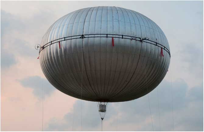
The multi-vectored propeller airship is a lighter-than-air aircraft with low flying speed, which has wide applications in earth observation( Reference Yang and Liu 1 ) and communication due to its capability of non-power station-keeping on resisting the gravity.( Reference Li, Nahon and Sharf 2 ) The most important three control types of the airship are station-keeping control, trajectory tracking control and path following control.( Reference Yang 3 ) In station-keeping control, the performance of the controller is greatly influenced by wind because the airship often has a large volume and it is lighter than air. However, it is difficult to improve its station-keeping performance if the wind disturbance is not properly considered. This paper aims to propose a composite station-keeping controller to deal with wind disturbance and thrust saturation.
The current methods dealing with wind disturbance have been developed during the past decade. First, it was handled by a stabilisation method, in which the wind is regarded as an external disturbance. The stability of the controller is guaranteed via its robustness, such as linear control,( Reference Schmidt 4 ) backstepping control( Reference Azinheira, Moutinho and De Paiva 5 ) and dynamic inversion control.( Reference Acosta and Joshi 6 ) However, it would be hard for the controller to maintain stability in a strong wind disturbance if this disturbance exceeds the maximum value that the controller can handle. The second method, a path following algorithm, was then put forward.( Reference Saiki, Fukao, Urakubo and Kohno 7 ) In this method, the station-keeping control was transformed into a path following control scheme by expressing the kinematics model in the wind field. Then the wind was not a strong disturbance since it was modelled. This method was adopted by Zheng et al.( Reference Zheng, Huo and Wu 8 ) and Hong et al.( Reference Hong, Lin and Lan 9 ) However, this method needs the wind speed usually estimated by an anemometer,( Reference Dorrington 10 ) leading to inevitable external hardware costs. Therefore, the third method, an observer-based one, was presented to estimate the wind speed. It can also estimate external disturbance and model uncertainties at low costs with relatively high accuracy. A wind observer based on kinematics was employed by Zheng et al.( Reference Zheng, Zhu, Shi and Wu 11 ) for a constant wind. And a nonlinear DOB was proposed by Chen et al.( Reference Chen, Ballance, Gawthrop and O’Reilly 12 ) for a slow time-varying disturbance. Liu et al.( Reference Liu, Chen and Andrews 13 ) adopted DOB in designing the control system for a helicopter. Other observers like sliding mode observer (its robustness is often guaranteed by the signum function( Reference Wang, Gao, Karimi, Shen and Fang 14 )), and some other observer-based methods were reviewed in Chen et al.’s work.( Reference Chen, Yang, Guo and Li 15 )
The main motivation of this paper is to propose an MPC( Reference Camacho and Bordons 16 )-based composite controller for a multi-vectored propeller airship. The controller consists of three modules: model predictive control, disturbance observer (DOB) and tracking differentiator. It can eliminate the wind effect and handle the thrust saturation. MPC is an advanced control algorithm including three essential modules: predictive model, receding horizon control and feedback correction. Recently, more and more attention has been paid to the MPC method, but few of them are proposed to the airship. MPC algorithm is promising in handling the system uncertainties, and thrust’s saturation as well. MPC often optimises a cost function at each sampling time. The optimisation is often solved by a quadratic programming(QP) algorithm or linear matrix inequality (LMI) method.( Reference Wang, Xia, Shen and Zhou 17 ) This algorithm can directly handle saturation. But it usually needs significant numbers of iteration in solving the QP, thus causing too much online computation, or causing conservation in solving LMI. The iterations can be avoided by an analytical control law of the explicit NMPC,( Reference Grancharova and Johansen 18 ) but thrust saturation cannot be considered at the same time. This implies the saturation cannot be handled by MPC without iteration. Therefore, in this paper, TD ( Reference Han 19 , Reference Han 20 ) is proposed to preserve the analytical control law (or reduce the workload of online computation) and handle the thrust’s amplitude saturation. In addition, the nonlinear DOB is implemented to estimate the wind disturbance.
The main contributions are as follows: (1) a new wind model is proposed by the mechanism analysis. Compared with the path following method which often models the wind in the kinematics, this paper considered the wind as the wind-induced aerodynamic force in the dynamics. (2) A novel saturation method using TD is adopted. The online computation burden is relieved, and no change is needed in the MPC analytical control law. (3) A better parameter design method of TD is proposed. A time-varying design parameter of TD is developed based on the dynamics model.
This paper is organised as follows. The model of the airship is first introduced. The controller design is then carried out. The controller stricture and the stability analysis are provided in the following section. Simulation results are given to demonstrate the validity of the proposed method. The conclusion and future works are given in the last section.
2.0 Airship model
The multi-vectored propeller airship (see in Fig. 1) has a Eulerian shape with four even-distributed propellers in its equatorial plane. The payload is suspended underneath its body by ropes.

Figure 1 (Colour online) Structure of multi-vectored propeller airship.
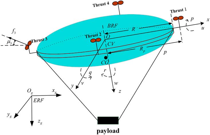
The earth reference frame (ERF) and body reference frame (BRF) are defined in Fig. 2, in which the states of the airship are also illustrated, where R is the radius of the airship, R
p
is the distance from the position of the propeller to volume center of the hull,
 $$[u\quad v\quad w]$$
stands for the linear velocities in BRF, and
$$[u\quad v\quad w]$$
stands for the linear velocities in BRF, and
 $$[p\quad q\quad r]$$
denotes the angular velocities in BRF.
$$[p\quad q\quad r]$$
denotes the angular velocities in BRF.

Figure 2 (Colour online) Frames and states of the airship.
2.1 Kinematics model of the airship
The kinematics models of the airship( Reference Chen and Duan 21 ) are
 $$\left[ {\matrix{ {\dot{x}_{g} } & {\dot{y}_{g} } & {\dot{z}_{g} } \cr } } \right]^{T} {\equals}{\bf{R}} _{{\mib{I}} }^{{\mib{B}} } \left[ {\matrix{ u & v & w \cr } } \right]^{T} $$
 $$\left[ {\matrix{ {\dot{\phi }} & {\dot{\theta }} & {\dot{\psi }} \cr } } \right]^{T} {\equals}{\bf{\Phi }} \left[ {\matrix{ p & q & r \cr } } \right]^{T} $$
 $$\openup 3pt{\bf R}_{{\mib{I}} }^{{\mib{B}} } {\equals}\left[ {\matrix{ {{\rm cos}\psi {\rm cos}\theta } & {{\rm cos}\psi {\rm sin}\theta {\rm sin}\phi {\minus}{\rm sin}\psi {\rm cos}\phi } & {{\rm cos}\psi {\rm sin}\theta {\rm cos}\phi {\plus}{\rm sin}\psi {\rm sin}\phi } \cr {{\rm sin}\psi {\rm cos}\theta } & {{\rm sin}\psi {\rm sin}\theta {\rm sin}\phi {\plus}{\rm cos}\psi {\rm cos}\phi } & {{\rm sin}\psi {\rm sin}\theta {\rm cos}\phi {\minus}{\rm cos}\psi {\rm sin}\phi } \cr {{\minus}{\rm sin}\theta } & {{\rm cos}\theta {\rm sin}\phi } & {{\rm cos}\theta {\rm cos}\phi } \cr } } \right]$$
where ϕ, θ, and ψ are the pitch, the yaw, and roll angles, respectively.
 $$[\matrix{ {x_{g} } & {y_{g} } & {z_{g} } \cr } ]$$
is the position in ERF.
$$[\matrix{ {x_{g} } & {y_{g} } & {z_{g} } \cr } ]$$
is the position in ERF.
 $${\mib{R}} _{{\mib{I}} }^{{\mib{B}} } $$
and Φ are the direction cosine transformation matrix and the angular transformation matrix, respectively. Using this two matrices, the velocity and the angular velocity are transferred from BRF to ERF. And both of them are detailed in (3) and (4)
$${\mib{R}} _{{\mib{I}} }^{{\mib{B}} } $$
and Φ are the direction cosine transformation matrix and the angular transformation matrix, respectively. Using this two matrices, the velocity and the angular velocity are transferred from BRF to ERF. And both of them are detailed in (3) and (4)
 $${\bf \Phi }{\equals}\left[ {\matrix{ 1 & {{\rm sin}\phi {\rm tan}\theta } & {{\rm cos}\phi {\rm tan}\theta } \cr 0 & {{\rm cos}\phi } & {{\minus}{\rm sin}\phi } \cr 0 & {{\rm sin}\phi {\rm sec}\theta } & {{\rm cos}\phi {\rm sec}\theta } \cr} } \right]$$
2.2 Dynamics model of the airship
The dynamics model under wind disturbance is
 $${\mib{M\vec{x}}} {\equals}{\mib{F}} _{{{\mib{GB}} }} {\plus}{\mib{F}} _{{\mib{A}} } {\plus}{\mib{F}} _{{\mib{w}} } {\plus}{\mib{F}} _{{\mib{I}} } {\plus}{\mib{F}} _{{\mib{T}} } $$
where M is the inertia matrix and F GB stands for the combined force of the buoyancy and the gravity. F A , F w , F I, and F T are the nominal aerodynamic force, the extra wind-induced aerodynamic force, the Coriolis force and the propeller force, respectively.
The mass matrix is presented as Equation (6), where I x , I y , I z , I xy , I xz , and I yz are the inertial moments of the airship. [x G , y G , z G ] is the position of gravity center. m is the total mass of the airship and payload, and m ii , i=1...6 are the added masses. The added mass is the inertia added to a system because when the vehicle is accelerated in a fluid, additional forces are required to increase the kinetic energy contained in the fluid. This effect appears as an apparent increase in the mass of the vehicle and is often referred to as added mass.( Reference Azinheira, De Paiva and Bueno 22 ) The value of the added masses can be calculated by the potential flow theory.More details can be seen in Wang’s work( Reference Wang 23 )
 $${\bf{M}} {\equals}\left[ {\matrix{ {m{\plus}m_{{11}} } & 0 & 0 & 0 & {mz_{G} } & {{\minus}my_{G} } \cr 0 & {m{\plus}m_{{22}} } & 0 & {{\minus}mz_{G} } & 0 & {m_{{26}} {\plus}mx_{G} } \cr 0 & 0 & {m{\plus}m_{{33}} } & {my_{G} } & {m_{{35}} {\minus}mx_{G} } & 0 \cr 0 & {{\minus}mz_{G} } & {my_{G} } & {I_{x} {\plus}m_{{44}} } & {{\minus}I_{{xy}} } & {{\minus}I_{{yz}} } \cr {mz_{G} } & 0 & {m_{{53}} {\minus}mx_{G} } & {{\minus}I_{{xy}} } & {I_{y} {\plus}m_{{55}} } & {{\minus}I_{{xz}} } \cr {{\minus}my_{G} } & {m_{{62}} {\plus}mx_{G} } & 0 & {{\minus}I_{{xz}} } & {{\minus}I_{{yz}} } & {I_{z} {\plus}m_{{66}} } \cr } } \right]$$
 $$\openup 3pt{\bf F}_{{{\bf GB}}} {\equals}\left[ {\matrix{ {{\minus}(G{\minus}B){\rm sin}\theta } \cr {(G{\minus}B){\rm sin}\phi {\rm cos}\theta } \cr {(G{\minus}B){\rm cos}\phi {\rm cos}\theta } \cr {{\minus}(Gz_{G} {\minus}Bz_{B} ){\rm sin}\phi {\rm cos}\theta } \cr {{\minus}(Gz_{G} {\minus}Bz_{B} ){\rm sin}\theta {\minus}(Gx_{G} {\minus}Bx_{B} ){\rm cos}\phi {\rm sin}\theta } \cr {(Gx_{G} {\minus}Bx_{B} ){\rm sin}\phi {\rm cos}\theta } \cr } } \right]$$
The combined force of the buoyancy and the gravity is presented in Equation (7). and [x B , y B , z B ] is the position of buoyancy center. G and B are the buoyancy and the gravity of the airship, respectively.
The Coriolis force is presented in Equation (8).
F A and F w are modeled in the next section.
 $$\openup 3pt{\bf F}_{{\bf I}} {\equals}\left[ {\matrix{ {{\minus}(m{\plus}m_{{33}} )wq{\plus}(m{\plus}m_{{22}} )vr{\minus}mz_{G} pr{\plus}mx_{G} (r^{2} {\plus}q^{2} ){\minus}my_{G} pq} \cr {{\minus}(m{\plus}m_{{11}} )ur{\plus}(m{\plus}m_{{33}} )wp{\minus}mz_{G} qr{\plus}my_{G} (r^{2} {\plus}p^{2} ){\minus}mx_{G} pq} \cr {{\minus}(m{\plus}m_{{22}} )vp{\plus}(m{\plus}m_{{11}} )uq{\minus}my_{G} qr{\plus}mz_{G} (p^{2} {\plus}q^{2} ){\minus}mx_{G} pr} \cr {(m_{{55}} {\minus}m_{{66}} {\minus}I_{z} {\plus}I_{y} )qr{\minus}my_{G} (pv{\minus}qu){\plus}mz_{G} (ru{\minus}pw)} \cr {(m_{{66}} {\minus}m_{{44}} {\minus}I_{x} {\plus}I_{z} )pr{\minus}mz_{G} (qw{\minus}rv){\plus}mx_{G} (pv{\minus}qu)} \cr {(m_{{44}} {\minus}m_{{55}} {\minus}I_{y} {\plus}I_{z} )qp{\minus}mx_{G} (ru{\minus}pw){\plus}my_{G} (qw{\minus}rv)} \cr } } \right]$$
2.3 Aerodynamic force model
If the airship works in an ideal circumstance and there exist no wind field during its operation, the aerodynamic force is defined as a nominal aerodynamic force. According to Liu,( Reference Liu 24 ) it can be presented as
 $$\openup 3pt{\mib{F}} _{{\mib{A}} } {\equals}\left[ {\matrix{ {{1 \over 2}\rho S_{{ref}} V^{2} C_{x} cos\varphi } \cr {{1 \over 2}\rho S_{{ref}} V^{2} C_{x} sin\varphi } \cr {{1 \over 2}\rho S_{{ref}} V^{2} C_{z} } \cr {{\minus}{1 \over 2}\rho S_{{ref}} L_{{ref}} V^{2} C_{{my}} sin\varphi {\minus}\xi _{p} p} \cr {{1 \over 2}\rho S_{{ref}} L_{{ref}} V^{2} C_{{my}} cos\varphi {\minus}\xi _{q} q} \cr {{1 \over 2}\rho S_{{ref}} L_{{ref}} V^{2} C_{{mz}} {\minus}\xi _{r} r} \cr } } \right]$$
where C
x
, C
z
, C
my,
and C
mz
are the aerodynamic coefficients. It can be observed that the aerodynamic coefficient in the x-axis and the y-axis is always the same, and also the rotation aerodynamic coefficient in the x-axis and the y-axis are the same, this is because the shape of the airship is symmetrical with respect to the z-axis. φ is the angle between the x-axis and the horizontal component of the inertial airship speed, so
 $${\rm tan}\varphi {\equals}{u \over v}$$
. ρ is the air density. S
ref
and L
ref
are the reference area and the length, respectively. The presentations are S
ref
=Vol
2/3 and L
ref
=Vol
1/3, where Vol is the volume of the airship. And
$${\rm tan}\varphi {\equals}{u \over v}$$
. ρ is the air density. S
ref
and L
ref
are the reference area and the length, respectively. The presentations are S
ref
=Vol
2/3 and L
ref
=Vol
1/3, where Vol is the volume of the airship. And
 $$V{\equals}\sqrt {u^{2} {\plus}v^{2} {\plus}w^{2} } $$
is the inertial airship speed in BRF, ξ
p
, ξ
q
, ξ
r
are the rotation damping coefficients. The damping coefficients are often proposed by the experience of the designer. In this paper, these are obtained by experiments.
$$V{\equals}\sqrt {u^{2} {\plus}v^{2} {\plus}w^{2} } $$
is the inertial airship speed in BRF, ξ
p
, ξ
q
, ξ
r
are the rotation damping coefficients. The damping coefficients are often proposed by the experience of the designer. In this paper, these are obtained by experiments.
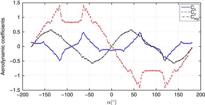
The aerodynamic coefficients are often obtained by wind-tunnel experiment, the symmetrical structure of the airship can help to reduce the cost of the experiment because the number of the coefficients is reduced. The wind-tunnel experiment is often conducted under different angle of attacks. In this paper, following Chen’s work,( Reference Chen, Zhang and Duan 25 ) the wind-tunnel experiment is conducted every 3° in [−180°,180°], and using linear interpolation, the coefficients of other angles are obtained. The results show that C mz ≈10−5 is close to zero and can be ignored, and C x , C z , C my are shown in Fig. 3.

Figure 3 (Colour online) Aerodynamic coefficients under different angle of attacks.
If the wind velocity is given as
 $$[u_{w} \quad v_{w} \quad w_{w} ]^{T} $$
, the real aerodynamic force can then be reconsidered. Define the wind-induced aerodynamic force as the difference between the real aerodynamic force and the nominal one, thus the wind-induced aerodynamic force can be presented as
$$[u_{w} \quad v_{w} \quad w_{w} ]^{T} $$
, the real aerodynamic force can then be reconsidered. Define the wind-induced aerodynamic force as the difference between the real aerodynamic force and the nominal one, thus the wind-induced aerodynamic force can be presented as
 $$\openup 3pt{\mib{F}} _{{\mib{w}} } {\equals}\left[ {\matrix{ {{1 \over 2}\rho S_{{ref}} \left( {V_{a}^{2} {\rm cos}\varphi _{w} {\minus}V^{2} {\rm cos}\varphi } \right)C_{x} } \cr {{1 \over 2}\rho S_{{ref}} \left( {V_{a}^{2} {\rm sin}\varphi _{w} {\minus}V^{2} {\rm sin}\varphi } \right)C_{x} } \cr {{1 \over 2}\rho S_{{ref}} \left( {V_{a}^{2} {\minus}V^{2} } \right)C_{z} } \cr {{\minus}{1 \over 2}\rho S_{{ref}} L_{{ref}} \left( {V_{a}^{2} {\rm sin}\varphi _{w} {\minus}V^{2} {\rm sin}\varphi } \right)C_{{my}} } \cr {{1 \over 2}\rho S_{{ref}} L_{{ref}} \left( {V_{a}^{2} {\rm cos}\varphi _{w} {\minus}V^{2} {\rm cos}\varphi } \right)C_{{my}} } \cr {{1 \over 2}\rho S_{{ref}} L_{{ref}} \left( {V_{a}^{2} {\minus}V^{2} } \right)C_{{mz}} } \cr } } \right]$$
where
 $$V_{a} {\equals}\sqrt {(u{\minus}u_{w} )^{2} {\plus}(v{\minus}v_{w} )^{2} {\plus}(w{\minus}w_{w} )^{2} } $$
is the airspeed and tanφ
w
=(u−u
w
)/(v−v
w
). φ
w
is the angle between the x-axis and the horizontal component of the airspeed.
$$V_{a} {\equals}\sqrt {(u{\minus}u_{w} )^{2} {\plus}(v{\minus}v_{w} )^{2} {\plus}(w{\minus}w_{w} )^{2} } $$
is the airspeed and tanφ
w
=(u−u
w
)/(v−v
w
). φ
w
is the angle between the x-axis and the horizontal component of the airspeed.
2.4 Propeller force model
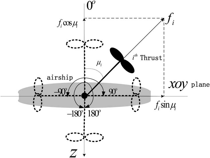
The propellers of the airship can be rotated in the vertical plane with a deflection angle μ i , and the propulsion forces are denoted by f i , i=1, 2, 3, 4. The detailed definition of deflection angle μ i can be seen in Fig. 4, the thrust can rotate in the range that μ i ∈[−180°,180°]. The deflection angle is 0 when the thrust is in the negative direction of the z-axis, the deflection angle is positive when the thrust rotates clockwise, and the deflection angle is negative when the thrust rotation is counterclockwise. These are the direct control variables given to the controller. In BRF, the thrust force is presented as
 $$\openup 3pt{\mib{F}} _{{\mib{T}} } {\equals}\left[ {\matrix{ {f_{2} {\rm sin}\mu _{2} {\minus}f_{4} {\rm sin}\mu _{4} } \cr {{\minus}f_{1} {\rm sin}\mu _{1} {\plus}f_{3} {\rm sin}\mu _{3} } \cr {{\minus}f_{1} {\rm cos}\mu _{1} {\minus}f_{2} {\rm cos}\mu _{2} {\minus}f_{3} {\rm cos}\mu _{3} {\minus}f_{4} {\rm cos}\mu _{4} } \cr {\left( {f_{4} {\rm cos}\mu _{4} {\minus}f_{2} {\rm cos}\mu _{2} } \right)R_{p} } \cr {\left( {f_{1} {\rm cos}\mu _{1} {\minus}f_{3} {\rm cos}\mu _{3} } \right)R_{p} } \cr {\left( {f_{1} {\rm sin}\mu _{1} {\plus}f_{2} {\rm sin}\mu _{2} {\plus}f_{3} {\rm sin}\mu _{3} {\plus}f_{4} {\rm sin}\mu _{4} } \right)R_{p} } \cr } } \right]$$

Figure 4 Definition of the deflection angle of the thrust.
Note in Equation (11), nonlinear couplings between f i and μ i are demonstrated, and control allocation must be conducted to obtain f i and μ i after F T is obtained, the control allocation is often completed by choosing a control allocation matrix. The chosen of the control allocation matrix is very important in dynamic inverse control allocation to avoid a singular value. Here, the indirect control vector u in is introduced as
 $${\mib{u}} _{{{\mib{in}} }} {\equals}[f_{1} {\rm sin}\mu _{1} ,\,f_{2} {\rm sin}\mu _{2} ,\,f_{3} {\rm sin}\mu _{3} ,\,f_{4} {\rm sin}\mu _{4} ,\,f_{1} {\rm cos}\mu _{1} ,\,f_{2} {\rm cos}\mu _{2} ,\,f_{3} {\rm cos}\mu _{3} ,\,f_{4} {\rm cos}\mu _{4} ]^{T} $$
This will result in a constant control allocation matrix. Thus, the inverse matrix is also a constant matrix, that is, a solution is always available in the control allocation process. Therefore, the propeller force is then decomposed as
 $${\mib{F}} _{{\mib{T}} } {\equals}{\mib{Bu}} _{{{\mib{in}} }} $$
the resulting control allocation matrix B is presented as
 $${\mib{B}} {\equals}\left[ {\matrix{ 0 & 1 & 0 & {{\minus}1} & 0 & 0 & 0 & 0 \cr {{\minus}1} & 0 & 1 & 0 & 0 & 0 & 0 & 0 \cr 0 & 0 & 0 & 0 & {{\minus}1} & {{\minus}1} & {{\minus}1} & {{\minus}1} \cr 0 & 0 & 0 & 0 & 0 & {{\minus}R_{p} } & 0 & {R_{p} } \cr 0 & 0 & 0 & 0 & {R_{p} } & 0 & {{\minus}R_{p} } & 0 \cr {{\minus}R_{p} } & {{\minus}R_{p} } & {{\minus}R_{p} } & {{\minus}R_{p} } & 0 & 0 & 0 & 0 \cr } } \right]$$
The direct control variables can then be solved by
 $$\eqalignno{ & f_{i} {\equals}\sqrt {\left( {f_{i} {\rm sin}\mu _{i} } \right)^{2} {\plus}\left( {f_{i} {\rm cos}\mu _{i} } \right)^{2} } \cr & \mu _{i} {\equals}{\rm arctan}{{f_{i} {\rm sin}\mu _{i} } \over {f_{i} {\rm cos}\mu _{i} }} $$
The dynamics equation can be transformed into a MIMO affine system. It is noted that in station-keeping control, the useful output is the position of the airship in ERF. Recall the dynamics model (5), the resulting affine system is
 $$\eqalignno{ & {\dot{\mib{x}}} {\equals}{\mib{f}} \left( {\mib{x}} \right){\plus}{\mib{g}} _{{\rm 1}} \left( {\mib{x}} \right){\mib{u}} _{{{\mib{in}} }} {\plus}{\mib{d}} \cr & {\mib{y}} {\equals}[x_{g} \quad y_{g} \quad z_{g} ]^{T} $$
where d = M −1 F w is the wind disturbance, g 1 ( x )= M −1 B , f ( x )= M −1( F GB + F A + F I ) and y is the system output.
3.0 The station-keeping controller
In this section, the station-keeping controller design procedure is carried out as follows. First, based on the work of Li et al.,( Reference Li, Yang, Chen and Chen 26 ) the explicit NMPC for station-keeping of the airship is derived, and nonlinear DOB is adopted for disturbance compensation. A saturation suppression strategy using TD is then put forward.
3.1 Explicit nonlinear MPC
For a nonlinear MIMO affine system such as the airship, it is well known that after continuously differentiating the output for a specific number of times, the control input appears in the expressions.
Definition 1. The number of times of differentiation required for the indirect control vector to appear is defined as the relative degree.
The relative degree is a vector, and for station-keeping control of the airship, it can be denoted as ρ r =[ρ r1, ρ r2, ρ r3]. Since the indirect control vector appears after some differentiations, the relative degree is first specified in the controller design. Before that, the following assumption is made to ensure the existence of these differentiations.
Assumption 1.
The states of the airship are all detectable, the output y and reference position
 $${\mib{w}} _{{\mib{d}} } {\equals}[x_{d} \quad y_{d} \quad z_{d} ]^{T} $$
are continuously differentiable.
$${\mib{w}} _{{\mib{d}} } {\equals}[x_{d} \quad y_{d} \quad z_{d} ]^{T} $$
are continuously differentiable.
Under Assumption 1, the relative degree and
 $${\mib{y}} ^{{[\rho _{r} ]}} $$
are obtained by the following differentiations.(
Reference Slegers and Costello
27
) The first derivative of
y
is the kinematics Equation (1).
$${\mib{y}} ^{{[\rho _{r} ]}} $$
are obtained by the following differentiations.(
Reference Slegers and Costello
27
) The first derivative of
y
is the kinematics Equation (1).
The second derivative of y is
 $$\left[ {\matrix{ {\ddot{x}_{g} } \cr {\ddot{y}_{g} } \cr {\ddot{z}_{g} } \cr } } \right]{\equals}{\bf R}_{{\mib{I}} }^{{\mib{B}} } \left[ {\matrix{ {\dot{u}{\plus}qw{\minus}rv} \cr {\dot{v}{\plus}ru{\minus}pw} \cr {\dot{w}{\plus}pv{\minus}qu} \cr } } \right]$$
Then
u
in
appears in the expression of
 $$\dot{u},\,\dot{v},\,\dot{w}$$
in Equation (5). Thus, the relative degree is ρ
r1=ρ
r2=ρ
r3=2.
$$\dot{u},\,\dot{v},\,\dot{w}$$
in Equation (5). Thus, the relative degree is ρ
r1=ρ
r2=ρ
r3=2.
Substituting Equation (15) into Equation (16) gives
 $$\left[ {\matrix{ {\ddot{x}_{g} } \cr {\ddot{y}_{g} } \cr {\ddot{z}_{g} } \cr } } \right]{\equals}{\bf R}_{{\mib{I}} }^{{\mib{B}} } {\mib{C}} \left( {{\mib{f}} \left( {\mib{x}} \right){\plus}{\mib{g}} _{{\rm 1}} \left( {\mib{x}} \right){\mib{u}} _{{{\mib{in}} }} {\plus}{\mib{d}} } \right){\plus}{\mib{F}} _{{{\mib{qw}} }} $$
where
 $${\mib{F}} _{{{\mib{qw}} }} {\equals}{\bf R}_{{\mib{I}} }^{{\mib{B}} } \left[ {qw{\minus}rv,\,ru{\minus}pw,\,pv{\minus}qu} \right]^{T} $$
and
$${\mib{F}} _{{{\mib{qw}} }} {\equals}{\bf R}_{{\mib{I}} }^{{\mib{B}} } \left[ {qw{\minus}rv,\,ru{\minus}pw,\,pv{\minus}qu} \right]^{T} $$
and
 $${\mib{C}} {\equals}\left[ {\matrix{ {{\mib{I}} _{{3{\times}3}} } & {{\mib{O}} _{{3{\times}3}} } \cr } } \right]$$
.
$${\mib{C}} {\equals}\left[ {\matrix{ {{\mib{I}} _{{3{\times}3}} } & {{\mib{O}} _{{3{\times}3}} } \cr } } \right]$$
.
Separating u in from Equation (17) gives
 $$\left[ {\matrix{ {\ddot{x}_{g} } & {\ddot{y}_{g} } & {\ddot{z}_{g} } \cr } } \right]^{T} {\equals}{\mib{L}} ({\mib{x}} ){\plus}{\bf R}_{{\mib{I}} }^{{\mib{B}} } {\mib{Cd}} {\plus}{\mib{A}} \left( {\mib{x}} \right){\mib{u}} _{{{\mib{in}} }} $$
where
 $${\mib{L}} \left( {\mib{x}} \right){\equals}{\bf R}_{{\mib{I}} }^{{\mib{B}} } {\rm (}{\mib{Cf}} {\rm (}{\mib{x}} {\rm )}{\plus}{\mib{F}} _{{{\mib{qw}} }} {\rm )}$$
and
$${\mib{L}} \left( {\mib{x}} \right){\equals}{\bf R}_{{\mib{I}} }^{{\mib{B}} } {\rm (}{\mib{Cf}} {\rm (}{\mib{x}} {\rm )}{\plus}{\mib{F}} _{{{\mib{qw}} }} {\rm )}$$
and
 $${\mib{A}} \left( x \right){\equals}{\bf R}_{I}^{B} {\mib{Cg}} _{1} ({\mib{x}} )$$
.
$${\mib{A}} \left( x \right){\equals}{\bf R}_{I}^{B} {\mib{Cg}} _{1} ({\mib{x}} )$$
.
Assumption 2. The system holds stable zero dynamics.
To achieve station-keeping of the airship, we need to design a controller such that the output y tracks the reference position w d . In MPC strategy, this can be achieved by minimising the following cost function:
 $${\mib{J}} {\equals}{\int}_0^{N_{p} } {\bf e}_{{\bf y}} \left( {t{\plus}\tau } \right)^{T} {\bf e}_{{\bf y}} \left( {t{\plus}\tau } \right)d\tau $$
where
 $${\bf e}_{{\bf y}} (t{\plus}\tau ){\equals}{\,\,\mib{{\vskip -3pt \hat}{\hskip -2pt y}}} (t{\plus}\tau ){\minus}{\,\,\mib{{\vskip -3pt \hat}{\hskip -3.5pt w}}} _{{\mib{d}} } (t{\plus}\tau )$$
, N
p
is the predictive horizon and 0≤τ≤
N
p
.
$${\bf e}_{{\bf y}} (t{\plus}\tau ){\equals}{\,\,\mib{{\vskip -3pt \hat}{\hskip -2pt y}}} (t{\plus}\tau ){\minus}{\,\,\mib{{\vskip -3pt \hat}{\hskip -3.5pt w}}} _{{\mib{d}} } (t{\plus}\tau )$$
, N
p
is the predictive horizon and 0≤τ≤
N
p
.
 $${\,\,\mib{{\vskip -3pt \hat}{\hskip -2pt y}}} (t{\plus}\tau )$$
, and
$${\,\,\mib{{\vskip -3pt \hat}{\hskip -2pt y}}} (t{\plus}\tau )$$
, and
 $${\,\,\mib{{\vskip -3pt \hat}{\hskip -3.5pt w}}} _{{\mib{d}} } (t{\plus}\tau )$$
are the approximations of the output and reference position at time t+τ respectively.
$${\,\,\mib{{\vskip -3pt \hat}{\hskip -3.5pt w}}} _{{\mib{d}} } (t{\plus}\tau )$$
are the approximations of the output and reference position at time t+τ respectively.
In general, the cost function is optimised by MPC to obtain
u
in
at each sampling time. In this paper,
 $${\,\,\mib{{\vskip -3pt \hat}{\hskip -2pt y}}} (t{\plus}\tau )$$
and
$${\,\,\mib{{\vskip -3pt \hat}{\hskip -2pt y}}} (t{\plus}\tau )$$
and
 $${\,\,\mib{{\vskip -3pt \hat}{\hskip -4pt w}}} _{{\mib{d}} } (t{\plus}\tau )$$
are approximated by Taylor series expansion up to
ρ
r
th order
$${\,\,\mib{{\vskip -3pt \hat}{\hskip -4pt w}}} _{{\mib{d}} } (t{\plus}\tau )$$
are approximated by Taylor series expansion up to
ρ
r
th order
The approximation using Taylor serial expansion of
 $${\,\,\mib{{\vskip -3pt \hat}{\hskip -2pt y}}} (t{\plus}\tau )$$
can be presented as
$${\,\,\mib{{\vskip -3pt \hat}{\hskip -2pt y}}} (t{\plus}\tau )$$
can be presented as
 $${\,\,\mib{{\vskip -4pt \hat}{\hskip -2pt y}}} (t{\plus}\tau ){\equals}\left[ {\matrix{ {x_{g} (t{\plus}\tau )} \cr {y_{g} (t{\plus}\tau )} \cr {z_{g} (t{\plus}\tau )} \cr } } \right]{\equals}\left[ {\matrix{ {x_{g} (t)} \cr {y_{g} (t)} \cr {z_{g} (t)} \cr } } \right]{\plus}\tau \left[ {\matrix{ {\dot{x}_{g} (t)} \cr {\dot{y}_{g} (t)} \cr {\dot{z}_{g} (t)} \cr } } \right]{\plus}{{\tau ^{2} } \over 2}\left[ {\matrix{ {\ddot{x}_{g} (t)} \cr {\ddot{y}_{g} (t)} \cr {\ddot{z}_{g} (t)} \cr } } \right]$$
To separate the unknown time parameter τ from the approximation, Equation (20) is rearranged as
 $${\,\,\mib{{\vskip -4pt \hat}{\hskip -2pt y}}} (t{\plus}\tau ){\equals}{\bf \Gamma } \left( \tau \right){\mib{Y}} \left( t \right)$$
where Γ(τ)=[
T
f
, Ts
],
 $${\mib{T}} _{{\bf s}} {\equals}diag\left[ {{{\tau ^{2} } \over 2},{{\tau ^{2} } \over 2},{{\tau ^{2} } \over 2}} \right]$$
,
T
f
=blkdiag ([1,τ], [1,τ], [1,τ]), it is the unkonwn matrix with the unknown τ.
$${\mib{T}} _{{\bf s}} {\equals}diag\left[ {{{\tau ^{2} } \over 2},{{\tau ^{2} } \over 2},{{\tau ^{2} } \over 2}} \right]$$
,
T
f
=blkdiag ([1,τ], [1,τ], [1,τ]), it is the unkonwn matrix with the unknown τ.
 $${\mib{Y}} \left( t \right){\equals}[{\mib{\bar{Y}}} _{1} \left( t \right),{\mib{\bar{Y}}} _{2} \left( t \right),{\mib{\bar{Y}}} _{3} \left( t \right),\ddot{x}_{g} ,\ddot{z}_{g} ,\ddot{z}_{g} ]^{T} ,$$
 $${\mib{\bar{Y}}} _{1} \left( t \right){\equals}[x_{g} ,\dot{x}_{g} ],{\mib{\bar{Y}}} _{2} \left( t \right){\equals}[y_{g} ,\dot{y}_{g} ]\!\,, {\mib{\bar{Y}}} _{3} \left( t \right){\equals}[z_{g} ,\dot{z}_{g} ].$$
Similar to
 $${\mib{\hat{y}}} \left( {t{\plus}\tau } \right),\,{\mib{\hat{w}}} _{{\mib{d}} } \left( {t{\plus}\tau } \right)$$
can be approximated as
$${\mib{\hat{y}}} \left( {t{\plus}\tau } \right),\,{\mib{\hat{w}}} _{{\mib{d}} } \left( {t{\plus}\tau } \right)$$
can be approximated as
 $${\mib{\hat{w}}} _{d} \left( {t{\plus}\tau } \right){\equals}{\bf \Gamma }\left( \tau \right){\mib{W}} _{d} \left( t \right)$$
where
 $${\mib{W}} _{d} \left( t \right){\equals}[{\mib{\bar{W}}} _{1} \left( t \right),{\mib{\bar{W}}} _{2} \left( t \right),{\mib{\bar{W}}} _{3} \left( t \right),\ddot{x}_{d} ,\ddot{y}_{d} ,\ddot{z}_{d} ]^{T} ,\,{\mib{\bar{W}}} _{1} \left( t \right){\equals}[x_{d} ,\dot{x}_{d} ],\,{\bf \bar{W}}_{3} \left( t \right){\equals}[z_{d} ,\dot{z}_{d} ],\,{\mib{\bar{W}}} _{2} \left( t \right){\equals}[y_{d} ,\dot{y}_{d} ],$$
Substituting Equations (21) and (22) into the Equation (19) gives
 $${\mib{J}} {\equals}\left[ {{\mib{Y}} \left( t \right){\minus}{\mib{W}} _{{\mib{d}} } \left( t \right)} \right]^{T} \left[ {\matrix{ {{\bf \Lambda }_{1} } & {{\bf \Lambda }_{2} } \cr {{\bf \Lambda }_{2}^{T} } & {{\bf \Lambda }_{3} } \cr } } \right]\left[ {{\mib{Y}} \left( t \right){\minus}{\mib{W}} _{{\mib{d}} } \left( t \right)} \right]$$
where
 $${\bf \Lambda }_{1} {\equals}{\int}_0^{N_{p} } {\mib{T}} _{{\mib{f}} } ^{T} {\mib{T}} _{{\mib{f}} } d\tau ,\,{\bf \Lambda }_{2} {\equals}{\int}_0^{N_{p} } {\mib{T}} _{{\mib{f}} } ^{T} {\bf T}_{{\mib{s}} } \left| {d\tau } \right.,\,{\bf \Lambda }_{3} {\equals}{\int}_0^{N_{p} } {\mib{T}} _{{\mib{s}} } ^{T} {\mib{T}} _{{\mib{s}} } d\tau .$$
Equation (23) can be minimised with respect to u in (t + τ). The necessary condition for the optimality is
 $${{\partial {\mib{J}} } \over {\partial {\mib{u}} _{{{\mib{in}} }} }}{\equals}{\rm 2}\left[ {{\mib{Y}} \left( {\mib{t}} \right){\minus}{\mib{W}} _{{\mib{d}} } \left( {\mib{t}} \right)} \right]^{T} \left[ {\matrix{ {{\mib{\Lambda }} _{{\mib{1}} } } & {{\mib{\Lambda }} _{{\mib{2}} } } \cr {{\mib{\Lambda }} _{{\mib{2}} }^{{\mib{T}} } } & {{\mib{\Lambda }} _{{\mib{3}} } } \cr } } \right]{{\partial {\mib{Y}} } \over {\partial {\mib{u}} _{{{\mib{in}} }} }}{\equals}0$$
Recall
Y
(t),
W
d
and define
 $${\mib{M}} _{{\rho _{r} }} {\equals}[{\mib{\bar{Y}}} _{1} {\minus}{\mib{\bar{W}}} _{1} \quad {\mib{\bar{Y}}} _{2} {\minus}\bar{W}_{2} \quad {\mib{\bar{Y}}} _{3} {\minus}{\mib{\bar{W}}} _{3} ]^{T} $$
, then Equation (24) can be
$${\mib{M}} _{{\rho _{r} }} {\equals}[{\mib{\bar{Y}}} _{1} {\minus}{\mib{\bar{W}}} _{1} \quad {\mib{\bar{Y}}} _{2} {\minus}\bar{W}_{2} \quad {\mib{\bar{Y}}} _{3} {\minus}{\mib{\bar{W}}} _{3} ]^{T} $$
, then Equation (24) can be
 $$2[{\mib{M}} _{{\rho _{r} }}^{T} \quad (\ddot{x}_{g} {\minus}\ddot{x}_{d} ,\ddot{y}_{g} {\minus}\ddot{y}_{d} ,\ddot{z}_{g} {\minus}\ddot{z}_{d} )]\,\left[ {\matrix{ {{\bf \Lambda }_{1} } & {{\bf \Lambda }_{2} } \cr {{\bf \Lambda }_{2}^{T} } & {{\bf \Lambda }_{3} } \cr } } \right]\,[{\rm 0}^{T} ,{\rm 0}^{T} ,{\mib{A}} ({\mib{x}} )^{T} ]^{T} {\equals}0$$
It gives that
 $${\mib{M}} _{{\rho _{r} }}^{T} {\bf \Lambda }_{2} {\plus}(\ddot{x}_{g} {\minus}\ddot{x}_{d} ,\ddot{y}_{g} {\minus}\ddot{y}_{d} ,\ddot{z}_{g} {\minus}\ddot{z}_{d} ){\bf \Lambda }_{3} {\equals}0$$
Recall Equation (18), and note Λ 3 is symmetrical, then the optimal control can be obtained by
 $${\mib{u}} _{{{\mib{in}} }} {\bf (}{\mib{t}} {\plus}\tau {\bf )}^{{\bf {\asterisk}}} {\equals}{\minus}{\mib{A}} \left( {\mib{x}} \right)^{{\plus}} \left[ {{\mib{KM}} _{{\rho _{r} }} {\plus}{\mib{M}} _{1} {\plus}{\mib{R}} _{I}^{B} {\mib{Cd}} } \right]$$
where
A
(
x
)
+
is the Moore–Penrose pseudoinverse of
 $${\mib{A}} \left( {\mib{x}} \right),{\mib{M}} _{1} {\equals} {\mib{L}} ({\bf x}){\minus}[\ddot{x}_{d} \quad \ddot{y}_{d} \quad \ddot{z}_{d} ]^{T} ,\,{\mib{K}} {\equals}{\bf \Lambda }_{3}^{{{\minus}1}} {\bf \Lambda }_{2}^{T} .$$
After solving the nonlinear equation (27), we can obtain the optimal control u in *(t+τ). In this paper, only the current control in the control profile is implemented. The explicit solution is u in *= u in (t+τ), for τ=0.
In addition, it can be noted that in Equation (27), the disturbance
d
is still unknown in the control law, so an observer is designed in the next section for disturbance rejection. After that,
d
is replaced by its estimation value
 $${\,\,\mib{{\vskip -5pt \hat}{\hskip -3pt d}}} $$
, then the influence of wind field is compensated. Therefore, the station-keeping control law is
$${\,\,\mib{{\vskip -5pt \hat}{\hskip -3pt d}}} $$
, then the influence of wind field is compensated. Therefore, the station-keeping control law is
 $${\mib{u}} _{{{\mib{in}} }} {\equals}{\minus}{\mib{A}} \left( {\mib{x}} \right)^{{\plus}} \left[ {{\mib{KM}} _{{\rho _{r} }} {\plus}{\mib{M}} _{1} {\plus}{\mib{R}} _{I}^{B} {\mib{C }{\,\,\mib{{\vskip -5pt \hat}{\hskip -3pt d}}} \right]$$
The direct control variables can then be calculated by Equation (14).
3.2 Nonlinear DOB
As disscused in the previous section, it is clear that
 $${\,\,\mib{{\vskip -5pt \hat}{\hskip -3pt d}}} $$
is indispensable in controller design. In this section, a nonlinear DOB is proposed to estimate the disturbance
$${\,\,\mib{{\vskip -5pt \hat}{\hskip -3pt d}}} $$
is indispensable in controller design. In this section, a nonlinear DOB is proposed to estimate the disturbance
 $${\mib{d}} $$
.
$${\mib{d}} $$
.
The nonlinear DOB for MIMO affine system (15) is designed as
 $$\eqalignno{ & {\dot{\mib{z}}} {\equals}{\minus}{\mib{l}} \left( {\mib{x}} \right){\mib{z}} {\minus}{\mib{l}} \left( {\mib{x}} \right)\left( {{\mib{p}} \left( {\mib{x}} \right){\plus}{\mib{f}} \left( {\mib{x}} \right){\plus}{\mib{g}} _{{\rm 1}} \left( {\mib{x}} \right){\mib{u}} _{{{\mib{in}} }} } \right) \cr & {\,\,\mib{{\vskip -5pt \hat}{\hskip -3pt d}}} {\equals}{\mib{z}} {\plus}{\mib{p}} \left( {\mib{x}} \right) $$
where z is the state vector of DOB, l ( x ) is the observer gain matrix, and p ( x ) is the nonlinear function to be designed. The observer gain matrix can be determined by
 $${\mib{l}} \left( {\mib{x}} \right){\equals}{{\partial {\mib{p}} \left( {\mib{x}} \right)} \over {\partial {\mib{x}} }}$$
Lemma 1. The DOB in (29) for system (15) is stable if the gain matrix l (x) is Hurwitz.
Proof. Define the estimation error as
 $${\mib{e{\equals}}} {\,\,\mib{{\vskip -5pt \hat}{\hskip -3pt d}}} {\minus}{\mib{d}} $$
. Then the differentiation of the estimation error with respect to time is
$${\mib{e{\equals}}} {\,\,\mib{{\vskip -5pt \hat}{\hskip -3pt d}}} {\minus}{\mib{d}} $$
. Then the differentiation of the estimation error with respect to time is
 $${\dot{\mib{e}}} {\equals} \,\, {{ \vskip -7pt \dot} \hskip 2pt{{\mib {{{\vskip -5pt \hat}}{\hskip -3pt d}}}}} &{\minus}{\dot{\mib{d}}}$$
Assumption 3.
The disturbance is slow time-varying
(
Reference Li, Yang, Chen and Chen
26
), so
 $${\dot{\mib{d}}} \,\approx\,$$
O
.
$${\dot{\mib{d}}} \,\approx\,$$
O
.
Substituting Equation (29) into Equation (31) gives
 $$\eqalignno{ {\dot{\mib{e}}} {\equals} {\,\,\mib{{\vskip -5pt \hat}{\hskip -3pt d}}} &{\equals}{\dot{\mib{z}}} {\plus}{{\partial {\mib{p}} \left( {\mib{x}} \right)} \over {\partial {\mib{x}} }}{\dot{\mib{x}}} \cr &{\equals}{\minus}{\mib{l}} \left( {\mib{x}} \right){\rm (}{\mib{z}} {\minus}{\dot{\mib{x}}} {\rm )}{\minus}{\mib{l}} \left( {\mib{x}} \right)\left( {{\mib{p}} \left( {\mib{x}} \right){\rm {\plus}}{\mib{f}} \left( {\mib{x}} \right){\rm {\plus}}{\mib{g}} _{{\rm 1}} \left( {\mib{x}} \right){\mib{u}} _{{{\mib{in}} }} } \right) $$
Substituting Equations (15) and (29) into Equation (32) gives
 $$\eqalignno{ \dot{e}&{\equals} {\minus}{\mib{l}} \left( {\mib{x}} \right){\rm (}{\,\,\mib{{\vskip -5pt \hat}{\hskip -3pt d}}} {\minus}{\mib{p}} \left( {\mib{x}} \right){\minus}{\mib{f}} \left( {\mib{x}} \right){\minus}{\mib{g}} _{{\mib{1}} } \left( {\mib{x}} \right){\mib{u}} _{{{\mib{in}} }} {\minus}{\mib{d)}} {\minus}{\mib{l}} \left( {\mib{x}} \right)\left( {{\mib{p}} \left( {\mib{x}} \right){\mib{{\plus}f}} \left( {\mib{x}} \right){\mib{{\plus}g}} _{{\mib{1}} } \left( {\mib{x}} \right){\mib{u}} _{{{\mib{in}} }} } \right) \cr &{\rm {\equals}}{\minus}{\mib{l}} \left( {\mib{x}} \right){\mib{e}} $$
This demonstrates that
 $${\,\,\mib{{\vskip -5pt \hat}{\hskip -3pt d}}} $$
approaches
d
exponentially if
l
(
x
) is Hurwitz.
$${\,\,\mib{{\vskip -5pt \hat}{\hskip -3pt d}}} $$
approaches
d
exponentially if
l
(
x
) is Hurwitz.
Remark 1. Although the stability analysis is carried out with Assumption 3, which is not often held in the realistic scenario. To the authors’ best knowledge, the DOB can also handle some time-varying disturbance, for example, sinusoidal disturbance and some small gust disturbances. These are verified in the simulation part.
3.3 Actuator saturation suppression based on TD
The amplitude of the propulsion force is severely limited in the realistic scenario, while the analytical control law (28) can handle no saturation. Therefore, to preserve the analytical control law and decrease the online computation burden, the TD employing time-varying design parameter is proposed.
Remark 2. MPC can also handle saturations, but usually through the use of a quadratic programming algorithm. The main drawback of MPC in handling saturation is the heavy computation load from iterations, no analytical control law and the difficulties in stability analysis. Compared with MPC, TD will not change the analytical law, thus no iteration exists.
TD is first proposed by Han,( Reference Han and Wang 28 ) and it uses a numerical method based on integrity to track the differentiation of the signal. In handling the saturation, TD always calculate a smooth govern path within the saturation. The main advantage of TD is the control of rapidness and strong robustness to the disturbance. The most common used TD( Reference Han 20 ) can be presented as
 $$\left\{ {\matrix{ {\dot{x}_{1} {\equals}x_{2} } \cr {\dot{x}_{2} {\equals}fhan\left( {x_{1} ,x_{2} ,R_{{TD}} } \right)} \cr } } \right.$$
where x 1 and x 2 are the states of the TD, they represent the position and velocity when respecting to the station-keeping control. R TD is the design parameter that represents the acceleration of the transition process. It is the only parameter that determines the transition time.( Reference Han and Yuan 29 ) fhan denotes the optimal control synthesis function. This function can avoid the chattering in steady state caused by the non-smooth structure of TD. It can be presented as
 $$fhan\left( {x_{1} ,x_{2} ,R_{{TD}} } \right){\equals}\left\{ {\matrix{ {R_{{TD}} a\quad \quad \,\mid\,a\,\mid\leq d_{t} } \cr {{\minus}R_{{TD}} {\rm sign}(a)\quad \quad \,\mid\,a\,\mid\gt\,d_{t} } \cr } } \right.$$
where d t =R TD h 0, h 0 is the sampling time interval, and a is presented as
 $$a{\equals}\left\{ {\matrix{ {x_{2} {\plus}c\,/\,h_{0} \quad \quad \,\mid\,c\,\mid\leq d_{{t0}} } \cr {x_{2} {\plus}sign(c)(a_{0} {\minus}d_{t} )\,/\,2\quad \quad \,\mid\,c\,\mid\,\gt\,d_{{t0}} } \cr } } \right.$$
where d
t0=d
t
h
0, c=x
1 + x
2
h
0 and
 $$a_{0} {\equals}\sqrt {d_{t}^{2} {\plus}8R_{{TD}} \,\mid\,c\,\mid\,^{2} } $$
.
$$a_{0} {\equals}\sqrt {d_{t}^{2} {\plus}8R_{{TD}} \,\mid\,c\,\mid\,^{2} } $$
.
To better understanding the basic theory and tracking performance of TD in path planning, the forward flight of the airship is taken as an example. The flight acceleration, transition time and reference position in the x-axis are defined as R
TD
, T
0, and x
d
, respectively. The acceleration has the shape of the square wave, and velocity having the triangle wave. To illustrate it in detail, in the first half of the process, the airship moves with a constant acceleration R
TD
, reaching the position
 $${{x_{d} } \over 2}$$
and velocity
$${{x_{d} } \over 2}$$
and velocity
 $${{T_{0} } \over 2}R_{{TD}} $$
. While in the latter half, the airship moves with the acceleration −R
TD
, reaching the position x
d
and velocity 0.
$${{T_{0} } \over 2}R_{{TD}} $$
. While in the latter half, the airship moves with the acceleration −R
TD
, reaching the position x
d
and velocity 0.
Figure 5 shows the position, velocity, and acceleration under different reference positions 10 m, 20 m, and 30 m, respectively, with R TD =0.5 m/s 2. It can be seen clearly that once the acceleration is determined, the controller will always achieve the same performance in handling the saturation, no matter how the reference positions change. Different reference positions will only lead to different transition times.
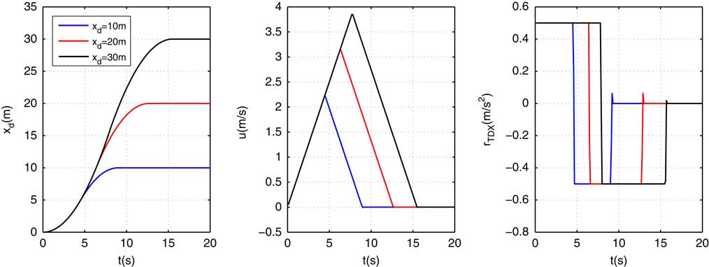
Figure 5 (Colour online) Path planning of TD.
In this paper, the main motivation of saturation handling strategy of TD is to choose a proper R TD so that the direct control variables will always be within its boundary. We propose a time-varying R TD choosing method based on the dynamics model of the airship via the relationship between the maximum flight acceleration and maximum propulsion force. Before that, the following assumption is made to simplify and decouple the dynamics model.
Assumption 4. In station-keeping control, the horizontal flight is considered, and the height of the airship remains constant.
Define *
max as the maximum value of *. Recall the dynamics model (5) and replace
d
by
 $${\mib{\hat{d}}} $$
. The maximum acceleration of the airship can be expressed by
$${\mib{\hat{d}}} $$
. The maximum acceleration of the airship can be expressed by
 $${\mib{M}} {\dot{\mib{x}}}_{{max}} {\equals}{\mib{F}} _{{{\mib{T}} max}} {\plus}{\mib{F}} _{{\mib{A}} } {\plus}{\mib{F}} _{{{\mib{GB}} }} {\plus}{\mib{F}} _{{\bf I}} {\plus}{\mib{M{\,\,\mib{{\vskip -5pt \hat}{\hskip -3pt d}}}} $$
Under Assumption 4, only the first two rows of Equation (37) are considered.
 $$\dot{p},\,\dot{q}\,{\rm and}\,\dot{r}$$
are not taken into consideration because of their small values. Define d
x
and d
y
as the disturbances in x- and y-axes,
$$\dot{p},\,\dot{q}\,{\rm and}\,\dot{r}$$
are not taken into consideration because of their small values. Define d
x
and d
y
as the disturbances in x- and y-axes,
 $$\hat{d}_{x} \,{\rm and}\,\hat{d}_{y} $$
as their estimations, respectively. Then the time-varying accelerations in x- and y-axes are
$$\hat{d}_{x} \,{\rm and}\,\hat{d}_{y} $$
as their estimations, respectively. Then the time-varying accelerations in x- and y-axes are
 $$\eqalignno{ & \left( {m_{0} {\plus}m_{{11}} } \right)\left( {\dot{u}_{{{\rm max}}} {\minus}\hat{d}x} \right){\equals}f_{{{\rm max}}} \left( {{\rm sin}\mu _{2} {\minus}{\rm sin}\mu _{4} } \right){\plus}{\mib{F}} _{{\mib{A}} } \left( 1 \right){\plus}{\mib{F}} _{{\bf I}} \left( 1 \right){\plus}{\mib{F}} _{{{\mib{GB}} }} \left( 1 \right) \cr & \left( {m_{0} {\plus}m_{{22}} } \right)\left( {\dot{v}_{{{\rm max}}} {\minus}\hat{d}y} \right){\equals}f_{{{\rm max}}} \left( {{\rm sin}\mu _{1} {\minus}{\rm sin}\mu _{3} } \right){\plus}{\mib{F}} _{{\mib{A}} } \left( 2 \right){\plus}{\mib{F}} _{{\mib{I}} } \left( 2 \right){\plus}{\mib{F}} _{{{\mib{GB}} }} \left( 2 \right) $$
Thus the maximum accelerations in x and y axes are
 $$\eqalignno{ & \dot{u}_{{max}} {\equals}{{f_{{max}} \left( {sin\mu _{2} {\minus}sin\mu _{4} } \right){\plus}{\mib{F}} _{{\mib{A}} } \left( 1 \right){\plus}{\mib{F}} _{{\mib{I}} } (1){\plus}{\mib{F}} _{{{\mib{GB}} }} \left( 1 \right)} \over {m0{\plus}m_{{11}} }}{\plus}\hat{d}_{x} \cr & \dot{v}_{{max}} {\equals}{{f_{{max}} \left( {sin\mu _{1} {\minus}sin\mu _{3} } \right){\plus}{\mib{F}} _{{\mib{A}} } \left( 2 \right){\plus}{\mib{F}} _{{\mib{I}} } {\plus}{\mib{F}} _{{{\mib{GB}} }} \left( {\bf 2} \right)\left( 2 \right)} \over {m_{0} {\plus}m_{{22}} }}{\plus}\hat{d}_{y} $$
Then
 $$\dot{u}_{{{\rm max}}} $$
and
$$\dot{u}_{{{\rm max}}} $$
and
 $$\dot{v}_{{{\rm max}}} $$
are used as the time-varying design parameters in Equation (34).
$$\dot{v}_{{{\rm max}}} $$
are used as the time-varying design parameters in Equation (34).
Remark 3.
The propulsion force may exceed its maximum value slightly for the reason that
 $$\dot{p},\,\dot{q}\,{\rm and}\,\dot{r}$$
are ignored. However, the saturation suppression can still be achieved by decreasing
$$\dot{p},\,\dot{q}\,{\rm and}\,\dot{r}$$
are ignored. However, the saturation suppression can still be achieved by decreasing
 $$\dot{u}_{{{\rm max}}} $$
and
$$\dot{u}_{{{\rm max}}} $$
and
 $$\dot{v}_{{{\rm max}}} $$
slightly.
$$\dot{v}_{{{\rm max}}} $$
slightly.
4.0 Controller structure and stability analysis
4.1 Controllerstructure
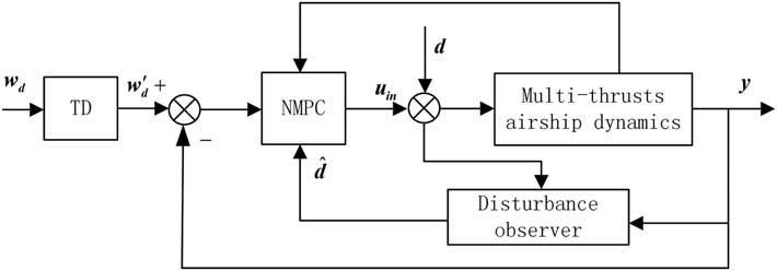
Based on the previous section, the station-keeping controller consists of three modules: explicit NMPC, nonlinear DOB, and TD. Its structure can be seen in Fig. 6.

Figure 6 Structure of the station-keeping controller.
In Fig. 6,
w
d
is the reference position of the station-keeping, and
 $${\mib{w'}} _{{\mib{d}} } {\equals}\left[ {\matrix{ {x'_{{d}} } & {y'_{{d}} } & {z'_{{d}} } \cr } } \right]^{T} $$
is the command position planned by TD, and the other parameters remain the same as previous.
$${\mib{w'}} _{{\mib{d}} } {\equals}\left[ {\matrix{ {x'_{{d}} } & {y'_{{d}} } & {z'_{{d}} } \cr } } \right]^{T} $$
is the command position planned by TD, and the other parameters remain the same as previous.
4.2 Stability analysis
From the structure of the controller, it can be seen that TD has no effect on the DOB-based NMPC controller. It only plans a command path in the station-keeping, so the stability relies on DOB and explicit NMPC. Now we focus on the stability of the DOB-based NMPC controller, and the stability analysis is given as follows.
Lemma 2. The station-keeping controller (28) for the system described in Equation (5), Equation (1) and Equation (2) is asymptotically stable if l(x) is Hurwitz and K is properly chosen.
Remark 4. The selection criterion of K is conducted in the following proof.
Proof. Compared with the conventional stability analysis, which often chooses a Lyapunov function,( Reference Wang, Shen, Karimi and Duan 30 ) this paper analysis the tracking error directly.
The position tracking error of station-keeping control is defined as
 $${\mib{z}} _{{\mib{p}} } ^{0} {\equals}\left[ {\matrix{ {x_{g} {\minus}x{\hbox{'}} _{d} } & {y_{g} {\minus}y \hbox{'} _{d} } & {z_{g} {\minus}z \hbox{'}_{d} } \cr } } \right]^{T} $$
Its first derivative is
 $${{\dot{\mib z}}} _{p}^{0} {\equals}{\mib{z}} _{{\mib{p}} } ^{1} {\equals}\left[ {\matrix{ {\dot{x}_{g} {\minus}\dot{x}\hbox{'}_{d} } & {\dot{y}_{g} {\minus}\dot{y} \hbox{'} _{d} } & {\dot{z}_{g} {\minus}\dot{z} \hbox{'} _{d} } \cr } } \right]^{T} $$
And the second derivative is
 $${{\dot{\mib z}}} _{{\mib{p}} }^{{\rm 1}} {\equals}\left[ {\matrix{ {\ddot{x}_{g} {\minus}\ddot{x} \hbox{'} _{d} } & {\ddot{y}_{g} {\minus}\ddot{y} \hbox{'} _{d} } & {\ddot{z}_{g} {\minus}\ddot{z} \hbox{'} _{d} } \cr } } \right]^{T} $$
Define
 $${\mib{z}} _{{\mib{p}} }^{{\rm 2}} {\equals}\left[ {\matrix{ {\ddot{x}_{g} } & {\ddot{y}_{g} } & {\ddot{z}_{g} } \cr } } \right]^{T} $$
Recall
 $$M_{{\rho _{r} }} $$
, M
1. Substituting Equations (18) and (28) into Equation (42) gives
$$M_{{\rho _{r} }} $$
, M
1. Substituting Equations (18) and (28) into Equation (42) gives
 $$\eqalignno{ {{\dot{\mib z}}} _{p}^{1} & {\equals} {\mib{M}} _{1} {\plus}{\mib{R}} _{I}^{B} {\mib{Cd}} {\plus}{\mib{A}} \left( {\mib{x}} \right)\left[ {{\minus}{\mib{A}} \left( {\mib{x}} \right)^{{\plus}} \left( {{\mib{KM}} _{{\rho _{r} }} {\plus}{\mib{M}} _{1} {\plus}{\mib{R}} _{{\mib{I}} }^{{\mib{B}} } {\mib{C{\,\,\mib{{\vskip -5pt \hat}{\hskip -3pt d}}}}} } \right)} \right] \cr &{\equals}{\minus}{\mib{KM}} _{{{\mib{\rho }} _{{\mib{r}} } }} {\mib{{\plus}R}} _{{\mib{I}} }^{{\mib{B}} } {\mib{Ce}} $$
where K =blkdiag ([k 11, k 12], [k 21, k 22], [k 31, k 32])
Recall
e
and
 $${\mib{z}} _{{\mib{p}} } ^{{\rm 2}} {{.\,\dot{\mib z}}} _{{\mib{p}} } ^{1} $$
can be expressed as
$${\mib{z}} _{{\mib{p}} } ^{{\rm 2}} {{.\,\dot{\mib z}}} _{{\mib{p}} } ^{1} $$
can be expressed as
 $${{\dot{\mib z}}} _{{\mib{p}} }^{{\mib{1}} } {\equals}{\mib{z}} _{{\mib{p}} } ^{2} {\plus}{\mib{R}} _{{\mib{I}} }^{{\mib{B}} } {\mib{Ce}} $$
Recall the presentation of
K
and
 $${\mib{M}} _{{\rho _{r} }} $$
, and rearrange them. Recall Equations (41), (42), and (45). The tracking error of the control system is
$${\mib{M}} _{{\rho _{r} }} $$
, and rearrange them. Recall Equations (41), (42), and (45). The tracking error of the control system is
 $$\left[ {\matrix{ {{\dot {\mib z}} _{{\mib{p}} }^{{\rm 0}} } \cr {{\dot {\mib z}} _{{\mib{p}} }^{{\rm 1}} } \cr } } \right]{\equals}\left[ {\matrix{ {{\rm 0}_{{3{\times}3}} } & {{\mib{I}} _{{3{\times}3}} } \cr {{\mib{K}} _{1} } & {{\mib{K}} _{2} } \cr } } \right]\left[ {\matrix{ {{\mib{z}} _{{\mib{p}} }^{{\rm 0}} } \cr {{\mib{z}} _{{\mib{p}} }^{{\rm 1}} } \cr } } \right]{\plus}\left[ {\matrix{ {{\rm 0}_{{3{\times}3}} } \cr {\epsilon} \cr } } \right]$$
where
K
i
=diag (k
1i
, k
2i
, k
3i
), i=1, 2,3, and
 $${\epsilon}{\equals}{\bf{R}} _{{\mib{I}} }^{{\mib{B}} } {\mib{Ce}} $$
.
$${\epsilon}{\equals}{\bf{R}} _{{\mib{I}} }^{{\mib{B}} } {\mib{Ce}} $$
.
The tracking error of the station-keeping controller can then be expressed as
 $${{\dot{\mib z}}} _{{\mib{p}} } {\equals}{\mib{f}} _{{\mib{A}} } {\mib{z}} _{{\mib{p}} } {\plus}{\epsilon}$$
From Lemma 1, we know that ϵ will converge to zeros if
l
(
x
) is Hurwitz. Therefore, the tracking error can be reduced to a linear system
 $${\dot{\mib{z}}} _{{\mib{p}} } {\equals}{\mib{f}} _{{\mib{A}} } {\mib{z}} _{{\mib{p}} } $$
, and its global asymptotic stability can be guaranteed by properly choosing
K
such that
$${\dot{\mib{z}}} _{{\mib{p}} } {\equals}{\mib{f}} _{{\mib{A}} } {\mib{z}} _{{\mib{p}} } $$
, and its global asymptotic stability can be guaranteed by properly choosing
K
such that
 $${{\mib{f}}_{{\mib{A}}$$
is Hurwitz. In this paper, it can be achieved by adjusting the predictive horizon such that
$${{\mib{f}}_{{\mib{A}}$$
is Hurwitz. In this paper, it can be achieved by adjusting the predictive horizon such that
 $${{\mib{f}}_{{\mib{A}}$$
is Hurwitz.
$${{\mib{f}}_{{\mib{A}}$$
is Hurwitz.
Remark 5.
If
 $${{\mib{f}}_{{\mib{A}}$$
is not Hurwitz by adjusting the predictive horizon, one other way to guarantee this condition can be described as follows: design a weighting matrix in the cost function (19), and then tuning the weighting matrix such that
$${{\mib{f}}_{{\mib{A}}$$
is not Hurwitz by adjusting the predictive horizon, one other way to guarantee this condition can be described as follows: design a weighting matrix in the cost function (19), and then tuning the weighting matrix such that
 $${{\mib{f}}_{{\mib{A}}$$
is Hurwitz.
$${{\mib{f}}_{{\mib{A}}$$
is Hurwitz.
5.0 SIMULATION RESULTS
In the following simulations, a multi-vectored propeller airship is used to analyze the proposed method.
The parameters needed in simulation are R=2.5 m, m
0=72 kg, Vol=70 m3, RP=2.55 m, ξp=ξq=200, ξr=100. The center of gravity is
 $$[x_{G} \quad y_{G} \quad z_{G} ]^{T} {\equals}[0\quad 0\quad 1.94]^{T} {\rm m}$$
. Other parameters needed are given in Table 1.
$$[x_{G} \quad y_{G} \quad z_{G} ]^{T} {\equals}[0\quad 0\quad 1.94]^{T} {\rm m}$$
. Other parameters needed are given in Table 1.
Table 1 Parameters of the multi-vectored propeller airship

The initial height of the airship in ERF is 100 m. The initial horizontal position is
 $$[0\quad 0]^{T} {\rm m}$$
. The reference horizontal position is
$$[0\quad 0]^{T} {\rm m}$$
. The reference horizontal position is
 $$[x_{d} \quad y_{d} ]^{T} {\equals}[20\quad 10]^{T} {\rm m}$$
and their derivatives are all zeros. The maximum propulsion force is f
max=500N. For simulation, the wind velocity is given as
$$[x_{d} \quad y_{d} ]^{T} {\equals}[20\quad 10]^{T} {\rm m}$$
and their derivatives are all zeros. The maximum propulsion force is f
max=500N. For simulation, the wind velocity is given as
 $$[10\quad 10\quad 0]{\rm m\,/\,s}$$
.
$$[10\quad 10\quad 0]{\rm m\,/\,s}$$
.
The design parameters
 $$\dot{u}_{{{\rm max}}} $$
and
$$\dot{u}_{{{\rm max}}} $$
and
 $$\dot{v}_{{{\rm max}}} $$
are calculated by Equation (39). The observer gain matrix of DOB is chosen as
l
(
x
)=
lx
, where l is a constant.
$$\dot{v}_{{{\rm max}}} $$
are calculated by Equation (39). The observer gain matrix of DOB is chosen as
l
(
x
)=
lx
, where l is a constant.
5.1 Parameters analysis of nonlinear DOB and explicit NMPC
In this section, the parameters l and N p are investigated. Some comparisons on the performance are carried out by applying different l and N p , and comments are given. Then the parameters with better performance are chosen for the next section to illustrate the effectiveness of the proposed station-keeping controller.
The DOB is first examined. The predictive horizon is given as N
p
=1 s. The estimation performances with different ls (1, 10, and 80) are given in Fig. 7. From lemma 1, we know that
 $$\hat{d}$$
approaches
d
exponentially if
l
(
x
) is Hurwitz. It means that the lager gain in DOB leads to faster converge rate. It is consistent with the simulation result in Fig. 7 (see when l=1 and l=10). When l increases, overshoot can be observed (see when l=80), but the converge rate does not change too much. Therefore, the tradeoff between overshoot and converge rate has to be made. Thus, l=10 is choosen.
$$\hat{d}$$
approaches
d
exponentially if
l
(
x
) is Hurwitz. It means that the lager gain in DOB leads to faster converge rate. It is consistent with the simulation result in Fig. 7 (see when l=1 and l=10). When l increases, overshoot can be observed (see when l=80), but the converge rate does not change too much. Therefore, the tradeoff between overshoot and converge rate has to be made. Thus, l=10 is choosen.
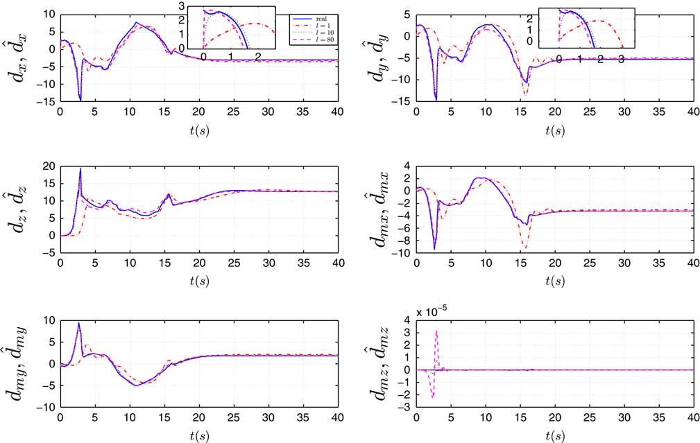
Figure 7 (Colour online) Disturbance observer performance under different l.
To verify remark 1, a random wind and a cosine wind field are also implemented in the simulation, and the parameters are l=10 and N p =1 s. The velocity of the random wind is given as [10 + 0.5ξ,10 + 0.5ξ,0] m/s, where ξ is a random value in [−1,1]. The cosine wind is given as [10 + sin(0.2t),10 + cos(0.2t),0] m/s. Figs. 8 and 9 show the results of the estimations. It can be seen that the estimations are both converged to the wind disturbance. The remark 1 is verified.
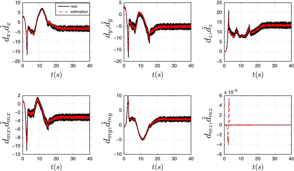
Figure 8 (Colour online) Disturbance observer performance of cosine wind.
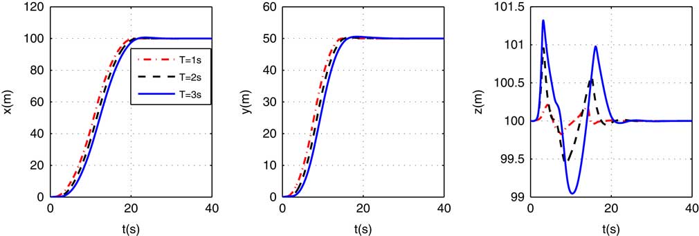
The explicit NMPC is then examined, and l=10 are fixed. The position responses under different N p s(1, 2, and 3 s) are given in Fig. 10. Figure 10 shows that the larger N p is, the larger the transition time of the system is. And larger predictive horizon also leads to larger overshoot( see in the z-axis). Thus, N p =1 s is chosen (Fig. 10).
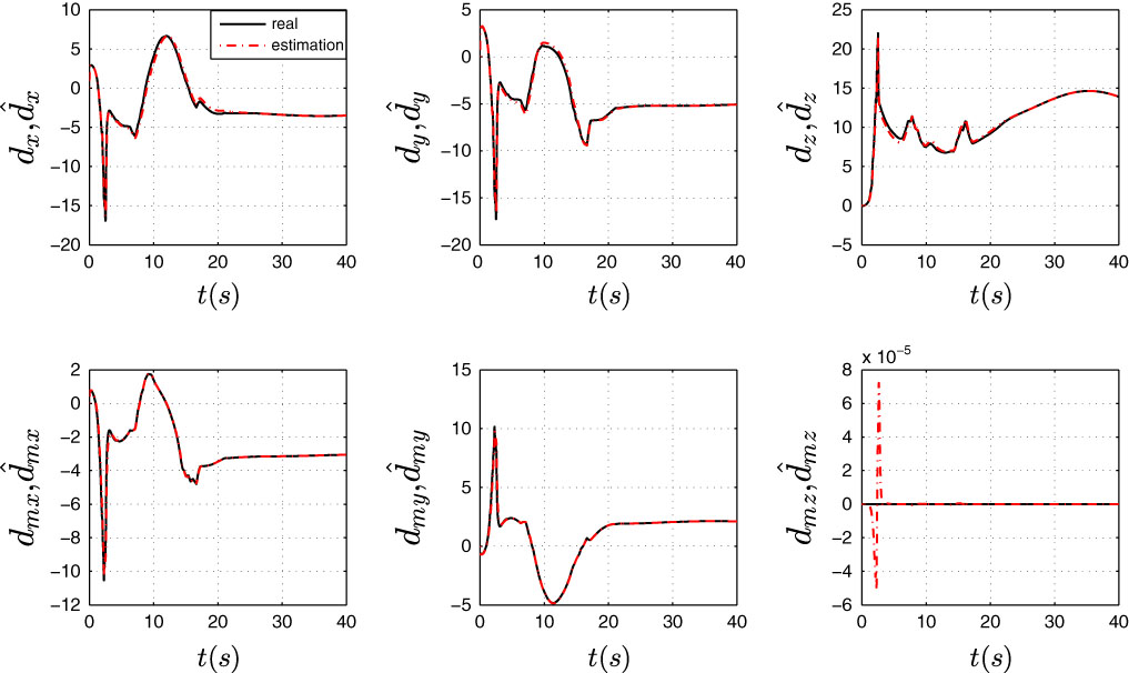
Figure 9 (Colour online) Positions under different predictive horizons.

Figure 10 (Colour online) Positions under different predictive horizons.
5.2 The controller performance
In this section, taking the wind disturbance and thrust saturation into consideration, we implement our method to the airship. According to the previous section, l=10 and N p =1 s are fixed in the following simulations.
The nonlinear DOB is illustrated with its ability for disturbance rejection. The states of the airship with or without nonlinear DOB are given in Fig. 11. The result shows that the controller with DOB performs much better. Specifically, the DOB can restrain the states’ variation degree, especially rolling angular velocity (its amplitude decreases significantly from 7.8 to 0.8 radians/s). It is able to drive the airship to the reference position (otherwise, the position of the airship cannot converge to the reference position). Since the disturbance is mainly caused by wind field, we can conclude that wind field (disturbance) has huge effects on the station-keeping performance. In addition, DOB has the ability of disturbance rejection, thus, the station-keeping performance has been significantly improved. Those interested in disturbance estimation performance can refer to Fig. 7 when l=10.
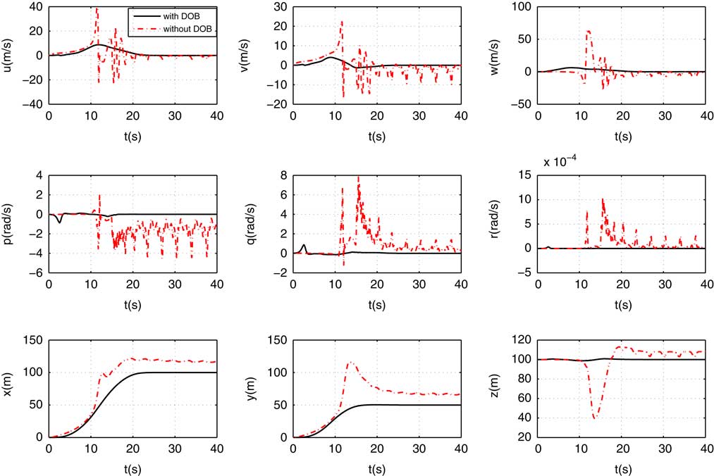
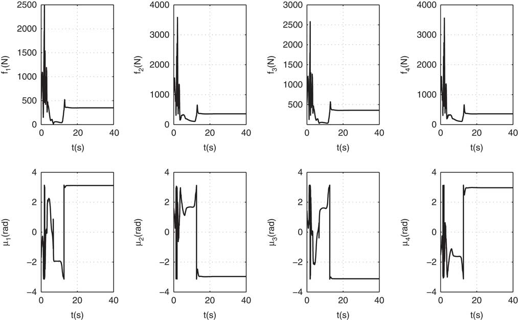
Figure 11 (Colour online) Velocities, angular velocities, and positions with or without nonlinear DOB.
Finally, the ability to handle the thrust saturation of TD is studied, and the propulsion forces and deflection angles are given in Fig. 12. The propulsion forces and deflection angles without using TD are given in Fig. 13 as a comparison. The two figures demonstrate that when the controller equipped with TD, the maximum value of propulsion forces decreases from 3685N (in propeller 4 at 5.8 s) to 502N (in propeller 3 at time 13.2 s). The propulsion force slightly exceeds the given maximum value. From the comparison, it can be concluded that the TD can handle thrust saturation efficiently.
Remark 6. One drawback of our method lies in the theory of TD. The current TD can only handle the amplitude saturation of the propulsion force. Problems occur if the saturation of changing rate is considered. The drawback could be discovered in Fig. 12 as some severe changes in the propulsion force can be observed. This could be mitigated by decreasing the design parameter of TD.

Figure 12 Propulsion forces and deflection angles with TD.

Figure 13 Propulsion forces and deflection angles without TD.
6.0 CONCLUSION
In this paper, a station-keeping control method is proposed by using the explicit NMPC framework. The controller can not only eliminate the influences of the wind field but also handle the saturation of the thrusts. It can also drive the airship to the desired reference position. Simulations based on a multi-vectored propeller airship are conducted and the ability of saturation suppression is revealed. The simulation results show that the proposed controller could successfully achieve the expected goals.
For future work, the problem of variation in the propulsion force and deflection angle is still to be solved. It is suggested that some saturation suppression strategies should be investigated, for example, taking the changing rate into consideration, so that the airship would not suffer much from severe changes in propeller force.
Acknowledgement
This work is supported by the National Science Foundation of China, No. 61733017 and 61703275, and by the Foundation of State Key Laboratory of Robotics of China, No. 2018O13, also sponsored by Shanghai Pujiang Program, No. 18PJD018.